
Submitted:
23 August 2023
Posted:
28 August 2023
You are already at the latest version
Abstract
This study explores the Edaravone solubility space encompassing both neat and binary dissolution media. The efforts were made toward revealing the concentration limits inherently associated with common pure and mixed solvents. For this purpose, the published solubility data of the title drug were scrupulously inspected and cured. This enabled to make the dataset consistent and coherent. However, the lack of some important types of solvents in the collection called for an extension of the available pool of Edaravone solubility data. Hence, new measurements were performed for collecting Edaravone solubility in polar non-protic and polar di-protic media. Such an extended set of data was used for tuning the parameters of regressors models and formulating the ensemble for predicting new data. In both phases, namely the model training and ensemble formulation, close attention was paid not only to minimizing the deviation of computed values from the experimental ones but also to ensuring the high predictive power and computing solubility for new systems. Furthermore, the environmental friendliness characteristics determined based on the common green solvent selection criteria was included in the analysis. Our applied protocol led to the conclusion that the solubility space defined by ordinary solvents is limited, and it is unlikely to find solvents that are more suited for Edaravone dissolution than those depicted in this manuscript. The theoretical framework presented in this study provides a precise guide for conducting experiments, saving time and resources in the pursuit of new findings.
Keywords:
edaravone
; solubility
; green solvents
; deep learning
; COSMO-RS
; learning curve analysis
; hyperparameters tuning
1. Introduction
Edaravone (5-methyl-2-phenyl-4H-pyrazol-3-one, EDA), as an active pharmaceutical ingredient (API), is used for the treatment of ischemic stroke [1,2] and amyotrophic lateral sclerosis (ALS) treatment [1,3]. These neuroprotective actions arise from the fact that Edaravone, being a free radical scavenger, has a serious anti-oxidant activity [4,5]. There is however an important limitation in the performance of Edaravone, namely its poor aqueous solubility, documented by its categorization as a Class IV drug in the Biopharmaceutics Classification System (BCS).
The solubility of chemical compounds plays a vital role in both theoretical and practical applications [6,7]. It affects various aspects such as reactivity, stability, and bioavailability of a compound when it can dissolve in a specific solvent. In the pharmaceutical industry, solubility holds significant importance in drug design and formulation [8,9,10]. Insufficient solubility can restrict a drug's effectiveness and its availability to the organism, resulting in higher expenses and reduced patient compliance. Hence, the development of proficient and successful techniques for assessing compound solubility remains of utmost significance [11,12,13,14]. In fact, the importance of solvents for the pharmaceutical industry is so profound that it can be estimated that they constitute up to 90% of the total volume of chemicals used during the drug manufacturing process [15].
In the case of Edaravone, its solubility was studied in aqueous binary solvents, mixed organic solvents, as well as neat solvents, including water [16,17,18]. Also our research group contributed to these efforts by studying the solubility of Edaravone in aqueous solutions of deep eutectic solvents [17]. The selection of an appropriate solvent in order to overcome the limited solubility of a particular API can be a tedious and difficult task. The number of experiments that can be performed is limited not only by such factors as laboratory time and financial aspects but also due to the ongoing trend of restricting the usage of chemicals in the framework of green chemistry [19,20,21]. It seems therefore, that a screening stage, utilizing different computational methods, is necessary before starting actual experiments [22,23,24,25]. Machine learning can offer valuable help in this process. For special attention deserves the application of machine learning for determining the solubility limits of pharmaceuticals [26].
The main goal of this paper is a presentation of the effectiveness of such an approach for exploring the extended space of solvents to screen for new solvents with experimental validation.
2. Results and Discussion
2.1. Solubility Dataset
The dataset characterizing Edaravone solubility is an accumulation of values collected from available literature sources augmented with a series of new measurements reported in this paper. There are three accounts documenting the temperature depended solubility of the titled compound in fifteen neat solvents including alcohols, esters, some aprotic solvents [16,18], and water [17]. Besides, nine binary solvents mixtures were used for EDA dissolution measurements [18] in the range of temperatures and using binary mixtures with a variety of compositions. It might seem that such a collection is extended enough for machine learning purposes, however a closer inspection reveals three fundamental problems, which are addressed in this study. First of all, one can notice serious divergences for some systems in reported solubility values. This inconsistency prohibits the direct use of such a collection for the training of models due to the introduced inherent noise in the dataset. This frequently occurring problem is intrinsic to diverse measurement protocols. Hence, such methodological divergences require careful consideration [27] prior to model formulation. Secondly, the solubility space is not represented uniformly due to different numbers of measurements for dissimilar temperature ranges and concentrations of solvents mixtures, which might over-represent those systems studied more extensively in the dataset. Finally, the main focus in solubility determination was narrowed to polar-protic solvents, with very limited non-protic or di-protic solvents representation. To address the first two issues the final collection was cured using commonly accepted model equations by fitting their parameters based on experimental mole fractions. Here, the three parameters van’t Hoff and Jouban-Acree equations were used for neat and binary solvents, respectively. Besides, temperature standardization was done for a uniform representation of solubility in the final dataset. In Figure 1 there are exemplified the results of the data curation for two selected neat solvents, which have been found as the most problematic. The complete list of experimental solubility data is provided in supporting materials (see section S2). As it can be directly inferred from the plots presented in Figure 1, there are not only incongruences in the solubility values but also in their temperature trends. It happened that the highest diversities were observed for EDA solubility measured in ethyl acetate. Since only an arbitrary decision would allow the rejection of either of measurement series, the final solubility dataset was constructed based on the predictions of van’t Hoff equation parametrized using all available experimental data. Besides, temperature normalization was adopted by accepting data between 0°C and 50°C with 5°C intervals. Hence, points marked with black diamonds constitute the solubility dataset. Fortunately, the majority of saturated systems of EDA studied experimentally suffered much smaller deviations, as detailed in supporting materials (see section S2.1.) and presented in Figure 1 are the worst extremes.
However, these two systems are very important from the perspective of solubility data curation in binary mixtures as frequently selected components of such complex solvents. Indeed, in Figure 2 there are presented exemplary plots characterizing EDA solubility measured at T=0°C and 40°C in binary solvents comprising either of the two solvents discussed above. All fitting results regarding binary solvents are presented in supplementary section S2.2.
There are two very important conclusions drawn from the content of Figure 2. First of all, the JA model performs very well for such systems for which the set of solvents compositions is extended enough. Fortunately, this is the case for the majority of systems, except for the ethyl acetate-methanol binary solvents mixture. In this case, the fitting results in precise back computed solubility data but probably failed for other compositions not studied experimentally. It seems very unlikely to expect such serious non-monotonous behavior of the solubility line and the observed trends should be attributed to the high flexibility of the JA equation rather than the physical phenomenon. The second important aspect is related to mentioned above incongruences in neat solvents solubility, especially pronounced at elevated temperatures. After standardization of solubility data for neat solvents the obtained values were used for binary mixtures impair plots at low-concentration regions. This is probably the main reason for the observed predictions done with the JA model. However, this is not the issue from the perspective of dataset curation, provided that only experimentally studied compositions are included. Indeed, the corresponding back computed values perfectly match experimental ones preserving the congruency of solubility determined in binary mixtures with neat solvents. Hence, in the final dataset, the solubility values for binary mixtures were included as computed from the JA model without concentration standardization.
All systems are characterized in supporting materials by providing the graphical representations of the solubility trends, the values of fitted parameters of applied models, and elementary statistical measures quantifying the fitting accuracy.
2.2. Extension of EDA Solubility Space with Neat Solvents
The solubility dataset obtained after data curation and standardization still needs some attention due to the limited diversity of included solvents. For extending the solubility space, new EDA solubility measurements were performed in a more diverse set of solvents. For this purpose, several neat solvents of polar-aprotic type were included, namely diglyme (DIG), triglyme (TIG), tetraglyme (TEG), dimethyl sulfoxide (DMSO), 1-methyl-2-pyrrolidone, (NMP), and 4-formylmorpholine (4FM). Besides, also polar di-protic solvents were taken into account by the inclusion of 2,4-dimethylphenol (DMP), 1,2-propanediol (PG), diethylene glycol (DG), triethylene glycol (TG), and 1,3-butanediol (BG). Additionally, since the solvent can affect the crystalline form of the solid and hence its thermodynamic properties, the solid residues obtained after the solubility determination procedure were analyzed by using DSC and FTIR-ATR techniques (see supplementary Figure S1.3.). The absence of significant differences between the thermograms and spectra recorded for the precipitates and the pure EDA, such as new phase transition peaks or absorption bands shifts related to the new hydrogen bonds formation, suggests that no polymorphic or pseudo-polymorphic transformation occurs under the applied experimental conditions.
When taking into account the solubility of Edaravone in neat polar-aprotic solvents, it can be concluded that it is DMSO that offers the highest dissolution potential among the studied solvents. At 25 °C the mole fraction solubility of EDA in these solvents is equal to xEDA = 7.57 ∙ 10−2, while at 40 °C the solubility is elevated to xEDA = 29.81 ∙ 10−2. DMSO is followed by TEG in terms of effectiveness, with EDA solubility amounting to xEDA = 4.63 ∙ 10−2 and xEDA = 21.21∙ 10−2 for 25 °C K and 40 °C, respectively. The solubility of Edaravone in other solvents is substantially smaller, however the general trend of solubility increase with raised temperature holds for all studied cases. The results are graphically depicted in Figure 3, along with values cured using the three parameters van’t Hoff model. Also a single di-protic solvent, namely DMP, was listed here. Detailed results can be found in supplementary Table S1.1.
2.3. Extension of EDA Solubility Space with Aqueous Binary Solvents
Apart from using neat polar solvents, both aprotic and di-protic, additional solubility experiments were conducted for aqueous binary solvents. These were created by mixing the four consider di-protic solvents with water in varying molar proportions. Quite often the addition of another solvent, for example water, can lead to a substantial solubility increase of a particular API compared to the neat solvent, which is described as a cosolvency effect [28,29]. Triethylene glycol (TG) was responsible for the highest solubility of EDA amounting to a molar fraction of xEDA = 2.75 ∙ 10−2 at 25 °C. Interestingly, the aqueous binary composition with the molar fraction of the organic solvent equal x2* = 0.9 offered even better EDA solubility with xEDA = 3.58 ∙ 10−2. Also for 1,3-butanediol (BG) – water and 1,2-propanediol (PG) – water mixtures this particular composition results in higher solubility compared to pure solvents. The only exception is the binary solvent containing diethylene glycol (DG), for which no so-called cosolvation effect was observed. The results are depicted in Figure 4, together with values cured using the three parameters van’t Hoff model. Details can be found in supplementary Table S1.2.
2.4. Machine Learnig Solubility Model
The machine learning was performed by training the set of 36 regression models, which were used for the ensemble definition based on the performance and predictability potential assessed on test and validation subsets not used during the training phase. It adheres to good practice to tune the parameters of the models on the training set and verify their effectiveness using a portion of the data that has not been seen before. This procedure increases the predictability of the trained models. Figure 5 shows a scatter plot of the models' characteristics, which enables the identification of three sets of regressors with similar efficiencies. It is worth emphasizing that due to the definition of the score function used during models’ parameters tuning, the results of learning curve analysis are used as a final evaluation approach rather than MAE or R2 themselves. For this purpose, the area under the curve (AUC) was determined for every regressor model with optimized parameters, for which the percentage of the sample is systematically increased from 50% up to 100% of the dataset.
The first set of regressors, denoted as set A, comprises commonly used machine learning models for regression problems. These models have different algorithms for learning the relationship between input and output variables, as well as varying levels of complexity and hyperparameters that need to be tuned. While all models excel at handling high-dimensional input data and continuous variables, they differ in their strengths and weaknesses in terms of their ability to handle different types of data and noise levels. For instance, support vector machines are often used for small datasets, while ensemble-based models like HistGradientBoostingRegressor, CatBoostRegressor, and XGBRegressor are preferred for larger datasets. By grouping these models based on their performance, one can assess their effectiveness in predicting solubility and identify the most suitable model for our dataset. The second set of regressors marked as B comprises models which are also commonly used for regression problems and have different algorithms, complexities, and hyperparameters that need to be tuned. One commonality among these models is their ability to handle continuous input and output variables, while some models can also handle high-dimensional input data. However, these models have different strengths and weaknesses in terms of their ability to handle noisy data and perform well on small or large datasets. For instance, GaussianProcessRegressor is known for its ability to model complex functions and handle small datasets, while ensemble-based models like BaggingRegressor, RandomForestRegressor, and AdaBoostRegressor are often used for larger datasets. By grouping these models based on their performance, we can evaluate their effectiveness in predicting solubility and determine the best model for our particular dataset. By grouping these models based on their performance, we can evaluate their effectiveness in predicting solubility and choose the best model for our specific dataset.
Using a set of models instead of relying on a single best one can offer several benefits. Firstly, it allows for the evaluation of the performance of multiple models by averaging their predictions. This takes advantage of the strengths of regressors from complementary models that can capture different aspects of the data, providing more robust predictions. Grouping models into subsets based on their predicting abilities provides additional validation of the overall performance by comparing both back computations and new predictions. The fact that the yielded mean values and standard deviations were very similar is a good prognostic for practical ensemble applications. Secondly, using a set of models can help to mitigate the risk of overfitting to a particular model architecture or hyperparameters, which can be a common issue when relying on a single best model. Therefore, using an ensemble of models can provide a more comprehensive and reliable approach for predicting solubility and other regression problems. Hence, the ensemble comprising all of the subsets is used for solubility computations of Edaravone in the extended set of neat and binary mixtures. The details of ensemble predictions, as well as contributions from all three subsets, are provided in supporting materials (see Excel file SM_models.xlsx). Also all hyperparameters tuned for corresponding repressors are provided.
In the caption of Figure 5, the regressors sets are ordered according to descending values of AUC for the validation set. It happened that the two best models take advantage of regression algorithms based on the Support Vector Machine (SVM) technique. Among the NuSVR (Nu Support Vector Regression) and SVR (Support Vector Regression), the former is generally considered more robust to outliers compared to SVR. The "nu" parameter in NuSVR controls the upper bound on the fraction of margin errors and support vectors. Adjusting this parameter enables the control of the trade-off between the number of support vectors and the errors allowed in the training set. SVR, on the other hand, penalizes points that lie outside the error bounds more heavily, which can make it more sensitive to outliers. The overall performance of the best model is presented in Figure 6. Similar characteristics of all other regressors included in the three subsets are presented in supporting materials (see Section S3).
2.5. The Solubility Space Characteristics
The main reason for ensemble model development is the extension of solubility space on systems not studied experimentally. This cannot be done using solely COSMO-RS predictions, which is clearly documented in Figure 7. The left panel presenting the correlation between computed and experimental solubility values suggests only a qualitative accuracy of this theoretical framework. On the contrary, a perfect match between estimated and measured solubility in the case of the ensemble can be observed. On the right panel predictions made using both theoretical approaches were assorted according to increasing values of solubility derived from the machine learning model. The region marked by a green rectangle corresponds to higher EDA solubility than the one achieved in dichloromethane (which was the most effective solvent studied experimentally) at ambient conditions. Additionally, the green circles identify solvents, which are supposed to be environmentally friendly according to US Environmental Protection Agency (EPA) classification [30] by estimation of the so-called environmental index (EI). This parameter includes several toxicological factors: human toxicity by inhalation (HTPInh), human toxicity by ingestion (HTPIng), aquatic toxicity (ATP), terrestrial toxicity (TTP), and physicochemical features related to ozone depletion (ODP), global warming (GWP), acid rain (AR), and photochemical oxidation (PCOP). However, when the latter factor is taken into account, EI is very high in the case of DMSO, which is commonly regarded as green. Furthermore, the other physicochemical parameters, namely ODP, GWP, and AR include all important atmospheric hazards related to the potential reactivity of the solvents. For the purposes of this study, all solvents with EI < 1.0 are regarded as green ones [31] and are marked by green circles in Figure 7. There are two main conclusions that can be inferred from both panels. First of all, there is very little space for solubility extensions by the application of new solvents, especially if the “greenness” criterion is imposed. Indeed, the top five ranked solvents pointed out by the ensemble model as the most suited for Edaravone are collected in Table 1. It is interesting to note that all these solvents belong to the class of polar aprotic solvents. The first three seem to be almost identically effective bearing in mind the values of the standard deviations. So, DMSO is supposed to fulfill the criterion of the highest solubility limit of EDA in a neat solvent. It is also unlikely that any binary mixture, except for the ones comprising DMSO, can offer higher solubility. This conclusion cannot be so definitely stated solely on COSMO-RS derived solubility, as clearly visible by the cloud of points within the green zone in Figure 7.
3. Materials and Methods
3.1. Materials
Edaravone (EDA, CAS Number: 89-25-8, MW = 174.20 g/mol) was supplied by Sigma Aldrich (Saint Louis, MO, USA) and its purity was ≥98%. The following compounds were used as solvents throughout the study: diglyme (DIG, CAS Number: 111-96-6), triglyme (TIG, CAS Number: 112-49-2), tetraglyme (TEG, CAS Number: 143-24-8), dimethyl sulfoxide (DMSO, CAS Number: 67-68-5), 1-methyl-2-pyrrolidone, (NMP, CAS Number: 872-50-4), 4-formylmorpholine (4FM, CAS Number: 4394-85-8), 2,4-dimethylphenol (DMP, CAS Number: 105-67-9 ), 1,2-propanediol (PG, CAS Number: 57-55-6), diethylene glycol (DG, CAS Number: 111-46-6), triethylene glycol (TG, CAS Number: 112-27-6), 1,3-butanediol (BG, CAS Number: 107-88-0), and methanol (CAS Number: 67-56-1). The above chemicals were also purchased from Sigma Aldrich and their purity was stated by the supplier as ≥98%. All chemicals were used as obtained without any initial procedures.
3.2. Solubility Measurements
To assess the solubility of EDA in various solvents, excess amounts of EDA were added to test tubes containing either specific solvents or a binary mixture containing the organic solvent and water in different molar proportions. The saturated solutions were then placed in an Orbital Shaker Incubator ES-20/60 from Biosan (Riga, Latvia) and incubated at various temperatures for 24 hours. Four temperature points, ranging from 25°C to 40°C with 5°C intervals, were used for the incubation. The incubator temperature was precisely adjusted to within 0.1 degrees, with a variance of 0.5 degrees during the 24-hour cycle. The samples were simultaneously mixed at 60 rev/min. Next, the samples were filtered using syringes equipped with PTFE filters with a pore size of 0.22 µm. To prevent precipitation due to temperature differences between the solutions and instruments, all test tubes, pipette tips, syringes, and filters were preheated. They were placed in the same incubator as the samples and heated to the same temperature before handling. This step was particularly crucial when dealing with elevated temperatures, as the temperature difference could be substantial. After filtration, small quantities of the obtained filtrate were diluted in test tubes containing methanol and measured spectrophotometrically. The density of each solution was measured by weighing a 1 ml volume in 10 ml volumetric flasks using an Eppendorf Reference 2 pipette (Hamburg, Germany) with a systematic error of 6 μl. The RADWAG AS 110 R2.PLUS analytical balance (Radom, Poland) with a precision of 0.1 mg was also used for this purpose. Solubility determination was conducted using the A360 spectrophotometer from AOE Instruments (Shanghai, China). Spectra were recorded in the wavelength range of 190 nm to 400 nm with a resolution of 1 nm. Methanol was used for both diluting the samples and the initial calibration of the spectrophotometer. The analytical wavelength was set at 243 nm, and the absorbance at this wavelength was used to determine the EDA concentration in the samples and subsequently calculate its mole fractions. To ensure accuracy, three separate measurements were performed, and the resulting values were averaged. The calibration curve for EDA was prepared by diluting an initial stock solution and measuring the resulting solutions' spectrophotometric properties at decreased concentrations. The molar concentrations of the measured solutions ranged from 0.0023 to 0.023 mg/ml. The relationship between the absorbance values at 243 nm and the solution concentration was described by a linear equation A = 85.603 × C - 0.0179, with high linearity denoted by the determination coefficient R2 equal to 0.9993.
3.3. Instrumental Analysis of Solid Residues
The dried solid residues obtained after the solubility determination procedure were subjected to Fourier transform infrared spectroscopy (FTIR) and differential scanning calorimetry (DSC) measurements. For this purpose, the Perkin Elmer Spectrum Two spectrophotometer (Waltham, MA, USA) equipped with an attenuated total reflection (ATR) device and DSC 6000 calorimeter from PerkinElmer (Waltham, MA, USA) were used. The calorimetric measurements were employing a heating rate of 5 K/min and a 20 mL/min nitrogen flow to create an inert atmosphere. The samples were placed in standard aluminum pans. The DSC apparatus was calibrated using indium and zinc standards prior to the measurements.
3.4. Solubility Data Curation
The datasets used for model development underwent curing and unification. All solubility data in neat solvents were analyzed using a simple thermodynamic model relying on the fundamental Van 't Hoff equation extended for the temperature dependence of the equilibrium constant by a polynomial fit [32]. The following equation
has three adjustable parameters, which values were computed by minimizing root mean square deviations (RMSD) between experimental and computed values. The collection of obtained parameters values for all analyzed systems (including literature data [16,17,18]), along with graphical lustrations, is provided in supporting materials (see section S2, Table S2.1, and Figure S2.1)
The solubility of EDA in binary mixtures also were prone to curation. For this purpose, the Jouyban-Acree model [33,34] was used as it was proven to be able adequately represent the spectrum of solution behavior from ideal to highly non-ideal systems [35]. This semi-empirical thermodynamic mixing model relies on a nearly ideal binary solvent/Redlich–Kister equation accounting for contributions from both two-body and three-body interactions [34]. The following adaptation was used for the purpose of this study:
where J0, J1, and J2 are adjustable parameters and represents the mole fraction of the first solvent in the initial binary mixture. The collection of all fitted values determined in this study and obtained from the literature is provided in supporting materials (see section S2, Table S2.2).
3.5. Model Development
For the purpose of exploring the solubility space of Edaravone, an extensive search for non-linear models was performed. The full hyperparameters tuning procedure was used for 36 regression models, which were chosen based on a variety of algorithms including linear models, boosting, ensembles, nearest neighbors, neural networks, and other types of regressors. A Python code was developed specifically for this study, and the search for the optimal parameters of each model was conducted using Optuna study, a freely available Python package for hyperparameter optimization [36]. The collection of the tuned models was formulated after 5000 minimization trials using TPE (Tree-structured Parzen Estimator) as a sampler of the search algorithm. TPE is known for being computationally efficient and uses a probability density function to model the relationship between hyperparameters and performance metrics. To evaluate the performance of each regression model, a custom score function was developed, which combines multiple metrics to take into account both the model's accuracy and ability to generalize. This scoring function was already discussed [31] and only a short note is provided here. In the present study, the training dataset was used for computations using a formula (3) that includes the mean squared error between the predicted and actual values of the target variable, as well as penalties on the number of positive values and outliers.
where is the value of the mean squared error between the predicted and actual values, is the number of positive values, number of outliers, and values are obtained from the learning curve analysis. The scoring function has two penalties on the number of positive values and outliers. The first penalty ensures that the predicted values are formally acceptable, as the models were trained against the values of solubility expressed as the logarithm of the mole fraction, which should always be positive. The second penalty directs the acceptance of models with as few outliers as possible, defined as values that exceed three times the standard deviation. The first two terms in the formula (3) were obtained from the learning curve analysis (LCA) of the scikit-learn 1.2.2 library [37] which provides information on the model's performance for different training set sizes. It is worth noting that LCA utilizes cross-validation (CV), which was set to a 5-fold CV of the training dataset. The first two contributions are obtained from the learning curve analysis, which provides information on the model's ability to generalize to new, unseen data. To perform the learning curve analysis, the sklearn.model_selection.learning_curve function from the scikit-learn library [7] was used. Due to its computational expense, only two-point computations were performed by including 50% to 100% of the total data. Overall, this approach allowed us to evaluate the performance of the models and identify the optimal training set size for each model. To assess the performance of the tuned models, a learning curve analysis (LCA) was conducted using 20 points computations. The values included in the custom loss function corresponded to the mean absolute error (MAE) values obtained at the largest training set size. By combining the two types of components, the custom loss function provided information on the model's accuracy and ability to generalize to new, unseen data The ensemble model (EM) was formed by selecting the subset of regression models with the lowest values for both criteria. The final predictions were obtained by averaging the predictions from the selected models. This approach allowed us to develop an ensemble of models that provided more robust and accurate predictions of solubility.
3.6. Molecular Descriptors
In order to develop a model for selecting effective EDA solubilizers, suitable molecular descriptors are to be selected. Selecting the molecular descriptors carrying sufficient structural information is a crucial step for the model development. Since the input data depend on the temperature, the quantum chemistry COSMO-RS method available in the COSMOtherm package [38] was applied [39] instead of typical QSPR/QSAR molecular features. The set of computed variables comprised intermolecular interaction descriptors, chemical potential, activities, solubility values, gas phase properties, σ-profiles and σ-potentials, σ-moments, and other features. Noteworthy, several previous studies have revealed the high predicting power of the COSMO-RS descriptors combined with machine learning techniques [17,27,40,41,42]. In order to develop the most reliable tool for solvent screening the sets of computed molecular descriptors were subjected to preselection according to the following inclusion criteria: (1) correlation with experimentally determined data, (2) sufficient variability, and (3) orthogonality [43].
Based on the previous studies [31,40], the COSMO-RS computed solubility values seem to be the first-choice descriptors. Although it is frequently used, it is generally known as only qualitatively accurate. There are several limitations of this approach, among which is the necessity of providing experimental values for fusion thermodynamics if solid-liquid equilibria (SLE) are the subject of interest. For many compounds there are available [44,45] values of melting temperatures, Tm, and fusion enthalpies, ΔHfus. Indeed, for EDA the following values are reported Tm=127°C [18,46] and ΔHfus= 29.61 kJ/mol [18]. However, the SLE equilibrium is generally defined by the following equation [47,48,49]:
where R is the gas constant, as is the solute activity in saturated systems and ΔCp stands for heat capacity change upon melting. This value is generally unavailable, but seems to be important [49,50] especially for temperature ranges far from the melting point, which is surely the case for SLE measurements. Some researchers argue [51,52] that ignoring this contribution, ΔCp=0, introduces an acceptable estimation due to the cancelation of errors in eq. (4). On the other hand, there is evidence that ΔCp≈ΔSfus≈ΔHfus·Tm-1 is a better choice [52,53]. For ensuring as high as possible accuracy of COSMO-RS solubility estimation, preliminary computations were performed for finding the value minimizing the overall mean average percentage error, MAPE, for the whole solubility dataset. Hence, several trials of solubility computations were performed for a broad range of heat capacity changes and the resulting correlation between MAPE and the values of ΔCp is plotted in Figure 8. It is interesting to see that performed tuning induces quite a small effect on the overall accuracy of solubility determined using COSMO-RS. The initial guess ΔCp≈ΔSfus≈ΔHfus·Tm−1=74.0 J(mol·K)-1 is very close to the optimized value ΔCp(opt)=61.59 J(mol·K)−1. Hence, the final set of solubilities taken for machine learning purposes corresponds to this latter value. All solubility computations were done by allowing the SLE solving by COSMOtherm software in order to avoid problems with the iterative protocol.
The second molecular descriptor selected for machine learning is the relative value of infinite dilution activity coefficient (IDAC), , defined as follows:
where the S symbol denotes either the neat solvent or the binary mixtures. In the latter case, the value is computed simply as a sum of neat solvent IDAC values weighted with the mole fraction composition of the mixture without solute.
The output files generated for the purpose of IDAC computations were used for extraction of the relative values of intermolecular interactions in the studied systems. Hence, inclusion criteria met the following energetic terms:
where int stands for the total, misfit, van der Waals, or hydrogen bonding contributions. Again, in the case of mixed solvents, the values were computed as a weighted sum of the solvents’ contributions.
The COSMO-RS theory introduced the concept of Taylor-series expansion of the σ-potential:
and the resulting quantities were termed σ-moments. The zero-order σ-moment, , is simply the molecular area of the EDA. The first σ-moment , is the negative charge of the compound. The second σ-moment, , is related to the screening charge of the system. The third and fourth σ-moments characterize σ-profile skewness and kurtosis, respectively. The COSMOtherm program allows for computing at most the sixth σ-moment and the last two have no simple meaning. For the purpose of this study, the inclusion criteria fulfilled third-, fifth-, and sixth-order σ-moments.
The successful calculation of all molecular descriptors with the aid of COSMOtherm [38] requires a proper representation of the molecular structure. This step is done only once and our database comprises tens of thousands of compounds prepared for using BP_TZVPD_FINE_21.ctd parametrization. This step is described in every paper dealing with COSMO-RS computations, so here it is only reminded that the COSMOconf program [54] was used for generating the most representative conformers and the geometries were optimized using Turbomole [55,56].
4. Conclusions
The study investigated the solubility of Edaravone both experimentally and theoretically. An effort was made for ensuring that the solubility data collection was representative and coherent. This is a crucial step for machine learning purposes aimed at noise reduction of the data used for model development. The main idea behind the whole project was to extensively explore the solubility space by taking Edaravone as an exemplary drug.
In the final word it is worth to emphasize that the ensemble of regression models developed in this study was tailored to the physicochemical properties of Edaravone solubility by tuning the values of their parameters to a restricted solubility set of this particular drug. While this approach may appear limited to a specific system, it still offers broad generalization potential. In machine learning development, there are generally two philosophies that are not necessarily mutually exclusive. The first one aims for generalization across a broad set of systems but requires a vast amount of experimental data. The second approach restricts itself to a narrowed range of systems but is more pragmatic by accepting the scarcity of available measurements. Both approaches share the common tenet of non-linear relationships between the target property and known features. Solubility is one such complex physicochemical property that is dependent on many solute-solvent-related interrelationships. In this study, we offer a balance between these two main attitudes with a pragmatic approach. Our Python code, which utilizes comprehensive parameter tuning, can be used to solve a variety of practical problems encountered in real-life screening. Our applied protocol led to the conclusion that the solubility space defined by ordinary solvents is limited, and it is unlikely to find solvents that are more suited for Edaravone dissolution than those depicted in this manuscript. This is not a negative or restrictive conclusion; on the contrary, it points out that this direction is not worth the effort, and focusing on other possibilities might be a better solution. The solubility space is vast and extensive, and one can consider many more potential systems than just common solvents if one is open to accepting new, designed solvents that take advantage of ion pairs. Indeed, such a direction was previously suggested [19], and this study further supports this lineage of future work.
The theoretical framework presented in this study, along with the previous work [31], provides a more precise guide for conducting experiments, saving time and resources in the pursuit of new findings.
Supplementary Materials
The following supporting information can be downloaded at the website of this paper posted on Preprints.org. (a) in document file: S1. New edaravone solubility data, S2. Solubility data curation, S3. Regressor models characteristics; (b) in excel file SM_models.xlsx molecular descriptors, tuner regressors parameters, their predictions and ensemble definition and prediction.
Author Contributions
Conceptualization, P.C.; methodology, P.C., validation, M.P., T.J. and P.C.; formal analysis, M.P., T.J. and P.C.; investigation, M.P., T.J., M.M., K.M. and P.C.; resources, M.P., T.J., M.M., K.M. and P.C.; data curation, P.C.; writing—original draft preparation, M.P., T.J. and P.C.; writing—review and editing, M.P., T.J. and P.C.; visualization, P.C.; supervision, P.C.; project administration, P.C. All authors have read and agreed to the published version of the manuscript.
Funding
This research received no external funding.
Institutional Review Board Statement
Not applicable.
Informed Consent Statement
Not applicable.
Data Availability Statement
All data supporting the reported results are available on request from the corresponding author.
Acknowledgments
Authors express our appreciation and acknowledgement for the technical support provided by Mr. Tomasz Miernik in setting up the Python infrastructure. Specifically, his assistance in configuring the local cluster was invaluable in achieving efficient model training.
Conflicts of Interest
The authors declare no conflict of interest.
Sample Availability
Not applicable.
References
- Drugbank Edaravone. Available online: https://go.drugbank.com/drugs/DB12243 (accessed on 28 November 2022).
- Watanabe, T.; Tahara, M.; Todo, S. The Novel Antioxidant Edaravone: From Bench to Bedside. Cardiovasc. Ther. 2008, 26, 101–114. [Google Scholar] [CrossRef]
- Bhandari, R.; Kuhad, A.; Kuhad, A. Edaravone: a new hope for deadly amyotrophic lateral sclerosis. Drugs of Today 2018, 54, 349. [Google Scholar] [CrossRef]
- Mao, Y.-F.; Yan, N.; Xu, H.; Sun, J.-H.; Xiong, Y.-C.; Deng, X.-M. Edaravone, a free radical scavenger, is effective on neuropathic pain in rats. Brain Res. 2009, 1248, 68–75. [Google Scholar] [CrossRef]
- Lin, M.; Katsumura, Y.; Hata, K.; Muroya, Y.; Nakagawa, K. Pulse radiolysis study on free radical scavenger edaravone (3-methyl-1-phenyl-2-pyrazolin-5-one). J. Photochem. Photobiol. B Biol. 2007, 89, 36–43. [Google Scholar] [CrossRef]
- Martínez, F.; Jouyban, A.; Acree, W.E. Pharmaceuticals solubility is still nowadays widely studied everywhere. Pharm. Sci. 2017, 23, 1–2. [Google Scholar] [CrossRef]
- Savjani, K.T.; Gajjar, A.K.; Savjani, J.K. Drug solubility: importance and enhancement techniques. ISRN Pharm. 2012, 2012, 195727. [Google Scholar] [CrossRef]
- Govender, R.; Abrahmsén-Alami, S.; Folestad, S.; Olsson, M.; Larsson, A. Enabling modular dosage form concepts for individualized multidrug therapy: Expanding the design window for poorly water-soluble drugs. Int. J. Pharm. 2021, 602, 120625. [Google Scholar] [CrossRef]
- Ting, J.M.; Porter, W.W.; Mecca, J.M.; Bates, F.S.; Reineke, T.M. Advances in Polymer Design for Enhancing Oral Drug Solubility and Delivery. Bioconjug. Chem. 2018, 29, 939–952. [Google Scholar] [CrossRef]
- Kawabata, Y.; Wada, K.; Nakatani, M.; Yamada, S.; Onoue, S. Formulation design for poorly water-soluble drugs based on biopharmaceutics classification system: Basic approaches and practical applications. Int. J. Pharm. 2011, 420, 1–10. [Google Scholar] [CrossRef]
- Grossmann, L.; McClements, D.J. Current insights into protein solubility: A review of its importance for alternative proteins. Food Hydrocoll. 2023, 137, 108416. [Google Scholar] [CrossRef]
- Sou, T.; Bergström, C.A.S. Automated assays for thermodynamic (equilibrium) solubility determination. Drug Discov. Today Technol. 2018, 27, 11–19. [Google Scholar] [CrossRef] [PubMed]
- Lu, W.; Chen, H. Application of deep eutectic solvents (DESs) as trace level drug extractants and drug solubility enhancers: State-of-the-art, prospects and challenges. J. Mol. Liq. 2022, 349, 118105. [Google Scholar] [CrossRef]
- Suwanwong, Y.; Boonpangrak, S. Molecularly imprinted polymers for the extraction and determination of water-soluble vitamins: A review from 2001 to 2020. Eur. Polym. J. 2021, 161, 110835. [Google Scholar] [CrossRef]
- Constable, D.J.C.; Jimenez-Gonzalez, C.; Henderson, R.K. Perspective on Solvent Use in the Pharmaceutical Industry. Org. Process Res. Dev. 2007, 11, 133–137. [Google Scholar] [CrossRef]
- Qiu, J.; Huang, H.; He, H.; Liu, H.; Hu, S.; Han, J.; Yi, D.; An, M.; Guo, Y.; Wang, P. Solubility Determination and Thermodynamic Modeling of Edaravone in Different Solvent Systems and the Solvent Effect in Pure Solvents. J. Chem. Eng. Data 2020, 65, 3240–3251. [Google Scholar] [CrossRef]
- Cysewski, P.; Jeliński, T.; Przybyłek, M. Intermolecular Interactions of Edaravone in Aqueous Solutions of Ethaline and Glyceline Inferred from Experiments and Quantum Chemistry Computations. Molecules 2023, 28, 629. [Google Scholar] [CrossRef]
- Li, R.; Yao, L.; Khan, A.; Zhao, B.; Wang, D.; Zhao, J.; Han, D. Co-solvence phenomenon and thermodynamic properties of edaravone in pure and mixed solvents. J. Chem. Thermodyn. 2019, 138, 304–312. [Google Scholar] [CrossRef]
- DeSimone, J.M. Practical approaches to green solvents. Science. 2002, 297, 799–803. [Google Scholar] [CrossRef]
- Cvjetko Bubalo, M.; Vidović, S.; Radojčić Redovniković, I.; Jokić, S. Green solvents for green technologies. J. Chem. Technol. Biotechnol. 2015, 90, 1631–1639. [Google Scholar] [CrossRef]
- Becker, J.; Manske, C.; Randl, S. Green chemistry and sustainability metrics in the pharmaceutical manufacturing sector. Curr. Opin. Green Sustain. Chem. 2022, 33, 100562. [Google Scholar] [CrossRef]
- König-Mattern, L.; Komarova, A.O.; Ghosh, A.; Linke, S.; Rihko-Struckmann, L.K.; Luterbacher, J.; Sundmacher, K. High-throughput computational solvent screening for lignocellulosic biomass processing. Chem. Eng. J. 2023, 452, 139476. [Google Scholar] [CrossRef]
- Gupta, Y.; Bhattacharyya, S.; Vlachos, D.G. Extraction of valuable chemicals from food waste via computational solvent screening and experiments. Sep. Purif. Technol. 2023, 316, 123719. [Google Scholar] [CrossRef]
- Vilas-Boas, S.M.; Cordova, I.W.; Kurnia, K.A.; Almeida, H.H.S.; Gaschi, P.S.; Coutinho, J.A.P.; Pinho, S.P.; Ferreira, O. Comparison of two computational methods for solvent screening in countercurrent and centrifugal partition chromatography. J. Chromatogr. A 2022, 1666, 462859. [Google Scholar] [CrossRef] [PubMed]
- González-Miquel, M.; Díaz, I. Green solvent screening using modeling and simulation. Curr. Opin. Green Sustain. Chem. 2021, 29, 100469. [Google Scholar] [CrossRef]
- Vermeire, F.H.; Chung, Y.; Green, W.H. Predicting Solubility Limits of Organic Solutes for a Wide Range of Solvents and Temperatures. J. Am. Chem. Soc. 2022, 144, 10785–10797. [Google Scholar] [CrossRef] [PubMed]
- Cysewski, P.; Jeliński, T.; Przybyłek, M. Application of COSMO-RS-DARE as a Tool for Testing Consistency of Solubility Data: Case of Coumarin in Neat Alcohols. Molecules 2022, 27, 5274. [Google Scholar] [CrossRef]
- Hatefi, A.; Jouyban, A.; Mohammadian, E.; Acree, W.E.; Rahimpour, E. Prediction of paracetamol solubility in cosolvency systems at different temperatures. J. Mol. Liq. 2019, 273, 282–291. [Google Scholar] [CrossRef]
- Chen, X.; Fadda, H.M.; Aburub, A.; Mishra, D.; Pinal, R. Cosolvency approach for assessing the solubility of drugs in poly(vinylpyrrolidone). Int. J. Pharm. 2015, 494, 346–356. [Google Scholar] [CrossRef]
- Harten, P.; Martin, T.; Gonzalez, M.; Young, D. The software tool to find greener solvent replacements, PARIS III. Environ. Prog. Sustain. Energy 2020, 39, e13331. [Google Scholar] [CrossRef]
- Cysewski, P.; Jeliński, T.; Przybyłek, M. Finding the Right Solvent: A Novel Screening Protocol for Identifying Environmentally Friendly and Cost-Effective Options for Benzenesulfonamide. Molecules 2023, 28, 5008. [Google Scholar] [CrossRef]
- Galaon, T.; David, V. Deviation from van’t Hoff dependence in RP-LC induced by tautomeric interconversion observed for four compounds. J. Sep. Sci. 2011, 34, 1423–1428. [Google Scholar] [CrossRef]
- Hwang, C.A.; Holste, J.C.; Hall, K.R.; Ali Mansoori, G. A simple relation to predict or to correlate the excess functions of multicomponent mixtures. Fluid Phase Equilib. 1991, 62, 173–189. [Google Scholar] [CrossRef]
- Acree, W.E. Mathematical representation of thermodynamic properties. Part 2. Derivation of the combined nearly ideal binary solvent (NIBS)/Redlich-Kister mathematical representation from a two-body and three-body interactional mixing model. Thermochim. Acta 1992, 198, 71–79. [Google Scholar] [CrossRef]
- Jouyban, A. Handbook of Solubility Data for Pharmaceuticals; CRC Press, 2009; ISBN 9781439804889.
- Akiba, T.; Sano, S.; Yanase, T.; Ohta, T.; Koyama, M. Optuna: A Next-generation Hyperparameter Optimization Framework. Proc. ACM SIGKDD Int. Conf. Knowl. Discov. Data Min. 2019, 2623–2631. [Google Scholar]
- Pedregosa, F.; Varoquaux, G.; Gramfort, A.; Michel, V.; Thirion, B.; Grisel, O.; Blondel, M.; Prettenhofer, P.; Weiss, R.; Dubourg, V.; et al. Scikit-learn: Machine Learning in Python. J. Mach. Learn. Res. 2011, 12, 2825–2830. [Google Scholar]
- Dassault Systèmes. COSMOtherm, Version 22.0.0, Dassault Systèmes, Biovia: San Diego, CA, USA, 2022.
- Klamt, A.; Schüürmann, G. COSMO: a new approach to dielectric screening in solvents with explicit expressions for the screening energy and its gradient. J. Chem. Soc. Perkin Trans. 2 1993, 799. [Google Scholar] [CrossRef]
- Cysewski, P.; Jeliński, T.; Przybyłek, M.; Nowak, W.; Olczak, M. Solubility Characteristics of Acetaminophen and Phenacetin in Binary Mixtures of Aqueous Organic Solvents: Experimental and Deep Machine Learning Screening of Green Dissolution Media. Pharmaceutics 2022, 14, 2828. [Google Scholar] [CrossRef] [PubMed]
- Cysewski, P.; Przybyłek, M.; Rozalski, R. Experimental and theoretical screening for green solvents improving sulfamethizole solubility. Materials (Basel). 2021, 14, 5915. [Google Scholar] [CrossRef]
- Cysewski, P.; Jeliński, T.; Cymerman, P.; Przybyłek, M. Solvent screening for solubility enhancement of theophylline in neat, binary and ternary NADES solvents: New measurements and ensemble machine learning. Int. J. Mol. Sci. 2021, 22. [Google Scholar] [CrossRef] [PubMed]
- Cramer, R.D.; Bunce, J.D.; Patterson, D.E.; Frank, I.E. Crossvalidation, Bootstrapping, and Partial Least Squares Compared with Multiple Regression in Conventional QSAR Studies. Quant. Struct. Relationships 1988, 7, 18–25. [Google Scholar] [CrossRef]
- Acree, W.; Chickos, J.S. Phase Transition Enthalpy Measurements of Organic and Organometallic Compounds. Sublimation, Vaporization and Fusion Enthalpies From 1880 to 2015. Part 1. C1-C10. J. Phys. Chem. Ref. Data 2016, 45, 033101. [Google Scholar]
- Acree, W.; Chickos, J.S. Phase Transition Enthalpy Measurements of Organic and Organometallic Compounds and Ionic Liquids. Sublimation, Vaporization, and Fusion Enthalpies from 1880 to 2015. Part 2. C11–C192. J. Phys. Chem. Ref. Data 2017, 46. [Google Scholar]
- Mojtahedi, M.M.; Javadpour, M.; Abaee, M.S. Convenient ultrasound mediated synthesis of substituted pyrazolones under solvent-free conditions. Ultrason. Sonochem. 2008, 15, 828–832. [Google Scholar] [CrossRef] [PubMed]
- Christian, S.D. Regular and Related Solutions: The Solubility of Gases, Liquids, and Solids( Hildebrand, Joel H; Prausnitz, John M.). J. Chem. Educ. 1971, 48, A562. [Google Scholar] [CrossRef]
- Hildebrand, J.H.; Prausnitz, J.M.; Scott, R.L. Regular and Related Solutions: The Solubility of Gases, Liquids, and Solids; Van Nostrand Reinhold: New York, NY, USA, 1970. [Google Scholar]
- Nordström, F.L.; Rasmuson, Å.C. Determination of the activity of a molecular solute in saturated solution. J. Chem. Thermodyn. 2008, 40, 1684–1692. [Google Scholar] [CrossRef]
- Neau, S.H.; Bhandarkar, S. V.; Hellmuth, E.W. Differential molar heat capacities to test ideal solubility estimations. Pharm. Res. 1997, 14, 601–605. [Google Scholar] [CrossRef]
- Przybyłek, M.; Kowalska, A.; Tymorek, N.; Dziaman, T.; Cysewski, P. Thermodynamic Characteristics of Phenacetin in Solid State and Saturated Solutions in Several Neat and Binary Solvents. Molecules 2021, 26, 4078. [Google Scholar] [CrossRef]
- Cysewski, P.; Przybyłek, M.; Kowalska, A.; Tymorek, N. Thermodynamics and intermolecular interactions of nicotinamide in neat and binary solutions: Experimental measurements and COSMO-RS concentration dependent reactions investigations. Int. J. Mol. Sci. 2021, 22, 7365. [Google Scholar] [CrossRef]
- Svärd, M.; Rasmuson, Å.C. (Solid + liquid) solubility of organic compounds in organic solvents – Correlation and extrapolation. J. Chem. Thermodyn. 2014, 76, 124–133. [Google Scholar] [CrossRef]
- Dassault Systèmes. COSMOconf, Version 22.0.0, Dassault Systèmes, Biovia: San Diego, CA, USA, 2022.
- Ahlrichs, R.; Bär, M.; Häser, M.; Horn, H.; Kölmel, C. Electronic structure calculations on workstation computers: The program system turbomole. Chem. Phys. Lett. 1989, 162, 165–169. [Google Scholar] [CrossRef]
- TURBOMOLE GmbH. TURBOMOLE, Version 7.6.0, TURBOMOLE GmbH: Karlsruhe, Germany, 2021.
Figure 1.
Results of data curation of EDA solubility in neat methanol and ethyl acetate using values measured by [a] Li, et al. [18], and [b] Qiu, et al. [16]. The consensus lines characterize fitting to the van’t Hoff equation and black diamonds define solubility data included in the final dataset.
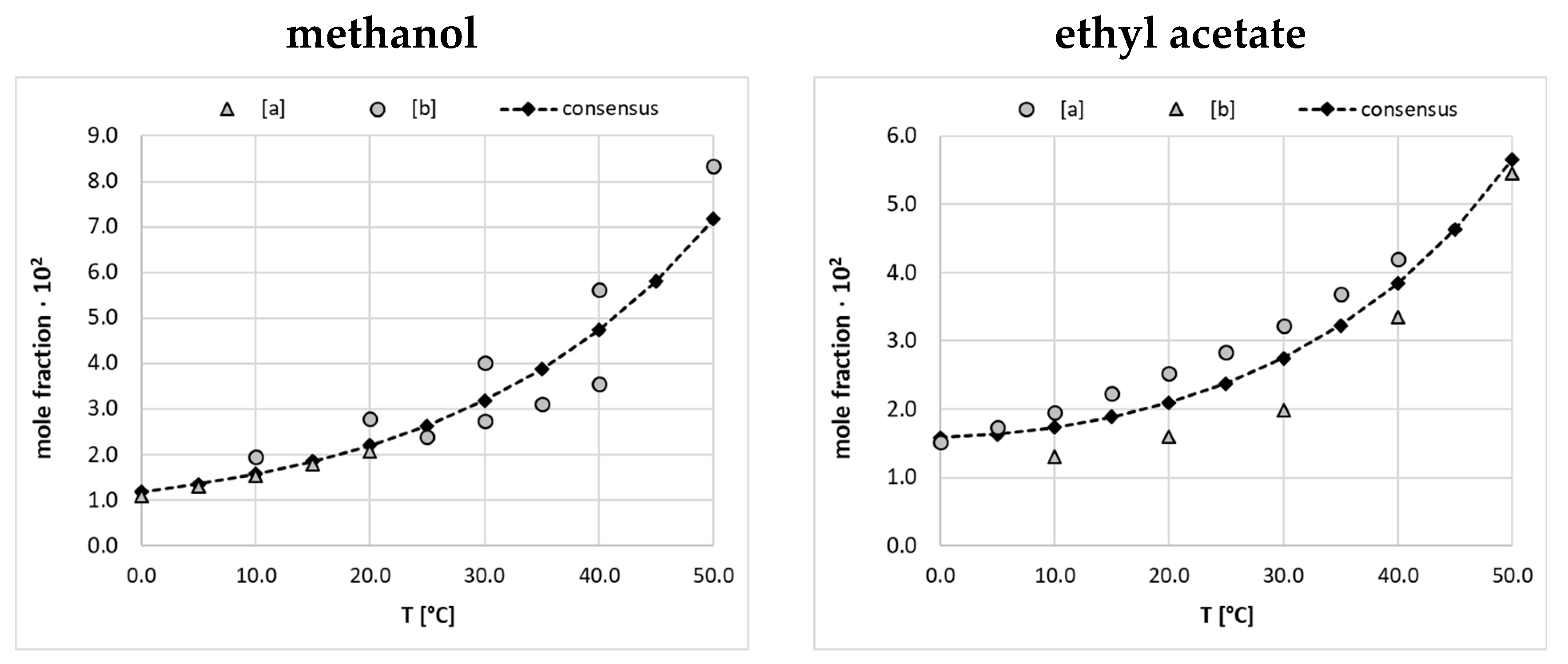
Figure 2.
Results of data curation of EDA solubility in exemplary binary solvents using values measured by Li, et al. [18]. The consensus lines characterize fitting to the Jouban-Acree equation and black diamonds define solubility data included in the final dataset.
Figure 2.
Results of data curation of EDA solubility in exemplary binary solvents using values measured by Li, et al. [18]. The consensus lines characterize fitting to the Jouban-Acree equation and black diamonds define solubility data included in the final dataset.
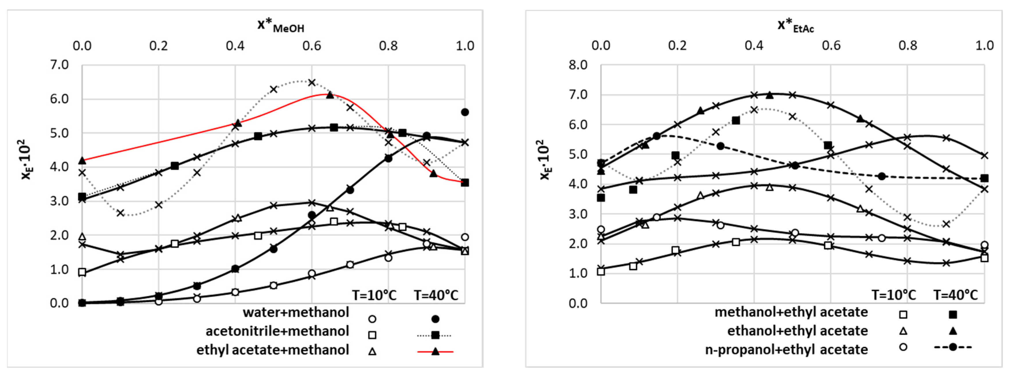
Figure 3.
Graphical representation of mole fraction solubility of Edaravone solubility in selected polar aprotic solvents. Gray and open symbols represent measured values and crosses depict cured values using the three parameters van’t Hoff model.
Figure 3.
Graphical representation of mole fraction solubility of Edaravone solubility in selected polar aprotic solvents. Gray and open symbols represent measured values and crosses depict cured values using the three parameters van’t Hoff model.
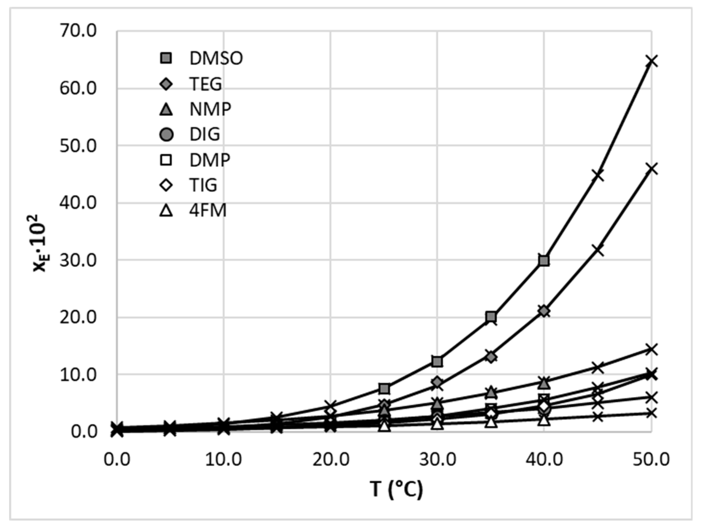
Figure 4.
Mole fraction solubility (at 30 °C) of Edaravone in aqueous binary mixtures of selected polar di-protic solvents. Gray and open symbols represent measured values and crosses depict cured values using three parameters JA model.
Figure 4.
Mole fraction solubility (at 30 °C) of Edaravone in aqueous binary mixtures of selected polar di-protic solvents. Gray and open symbols represent measured values and crosses depict cured values using three parameters JA model.
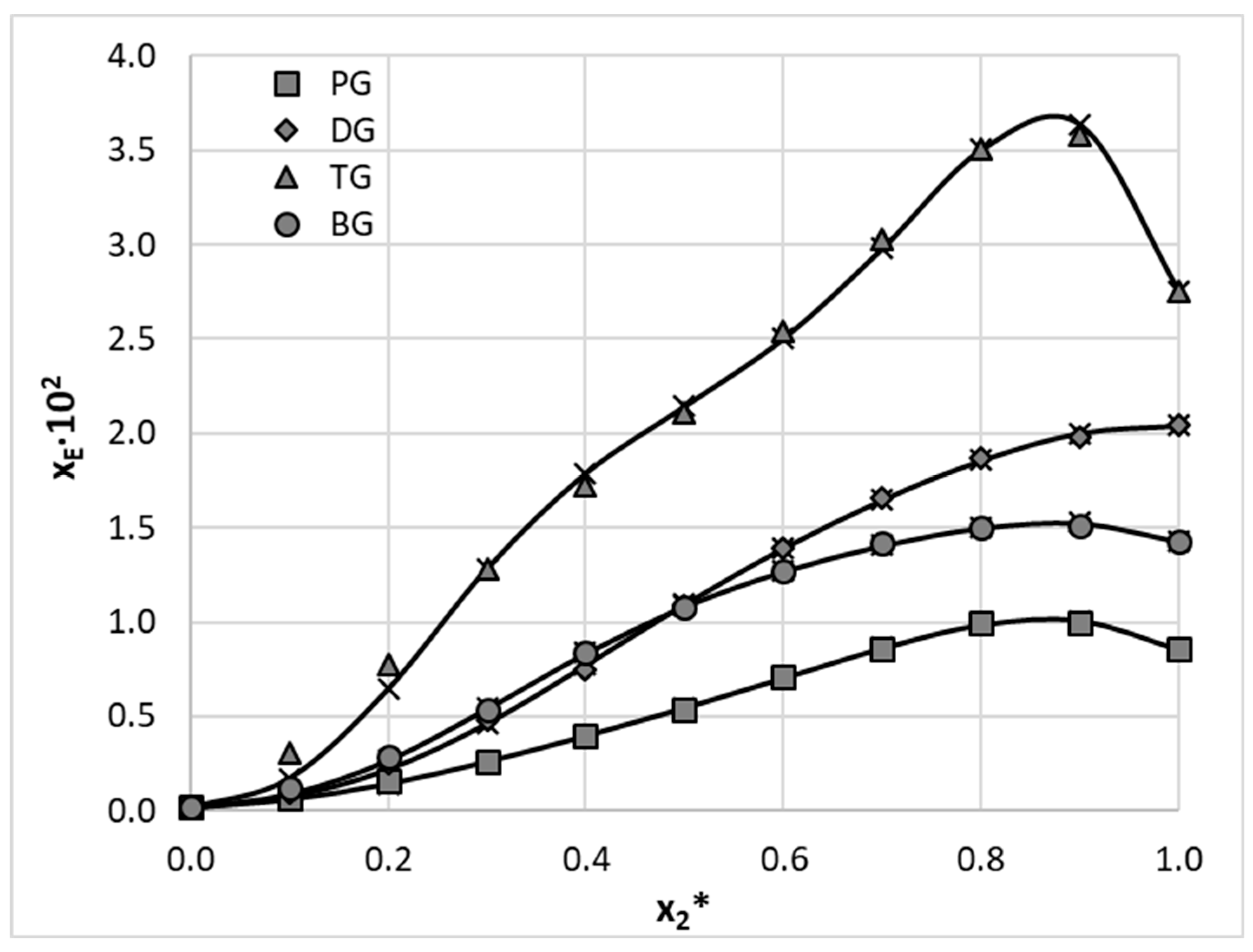
Figure 5.
Results of regression models’ selection based on the distributions of area under the AUC curve determined from learning curve analysis, loss values of test, and validation sets. The set A comprises the following five models: NuSVR, SVR, CatBoostRegressor, XGBRegressor, and HistGradientBoostingRegressor. In the set B there were categorized additionally twelve regressors including GaussianProcessRegressor, BaggingRegressor, RandomForestRegressor, LGBMRegressor, MLPRegressor, LassoLars, LassoLarsCV, Ridge, KNeighborsRegressor, AdaBoostRegressor, OrthogonalMatchingPursuitCV, and TransformedTargetRegressor.
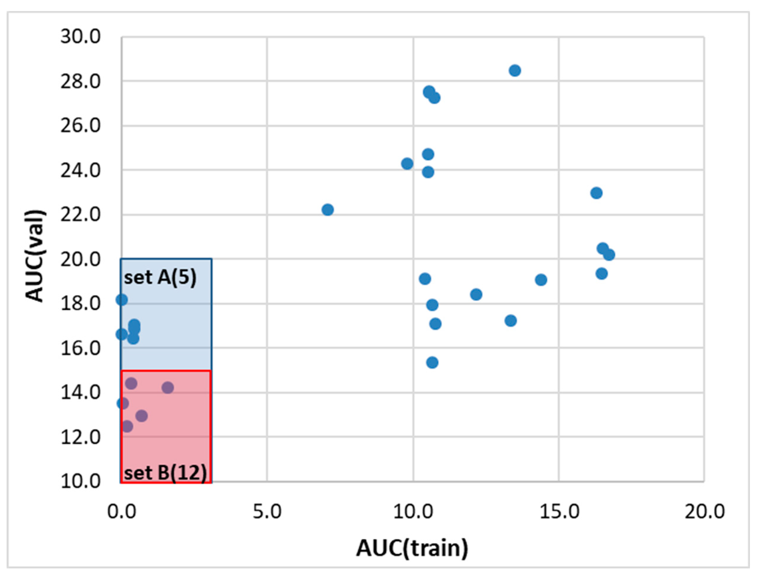
Figure 6.
Graphical illustration of the NuSVR regression model performance. The panels a, b, and c document the correlation between computed and consensus solubility values with annotation of the standard deviation as circles radius, applicability domain plots, and results of learning curve analysis concerning both R2 and MAE, respectively.
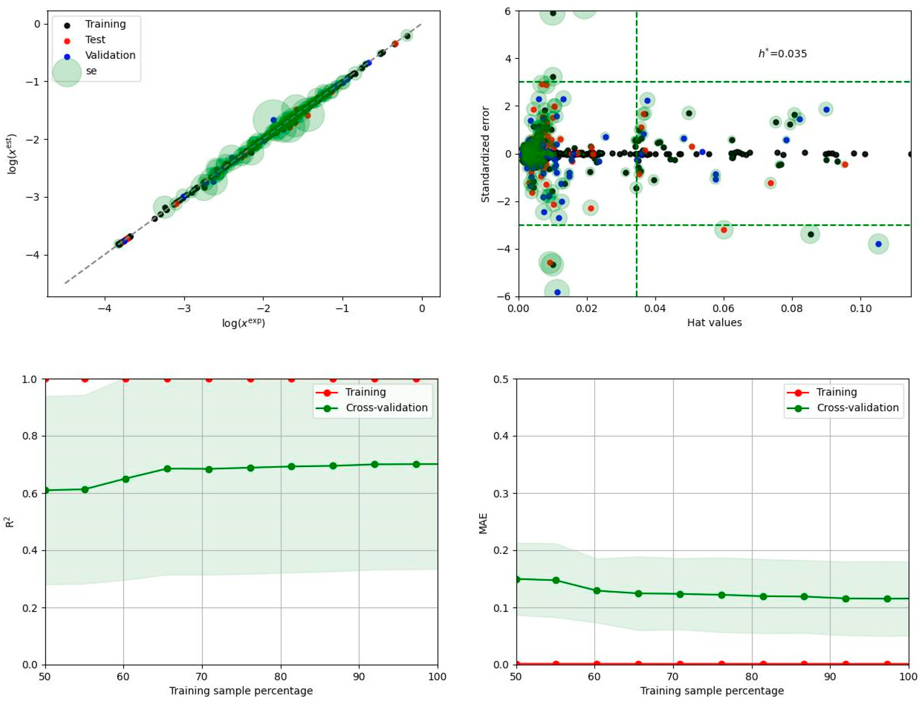
Figure 7.
The experimentally and theoretically determined solubility values of EDA.
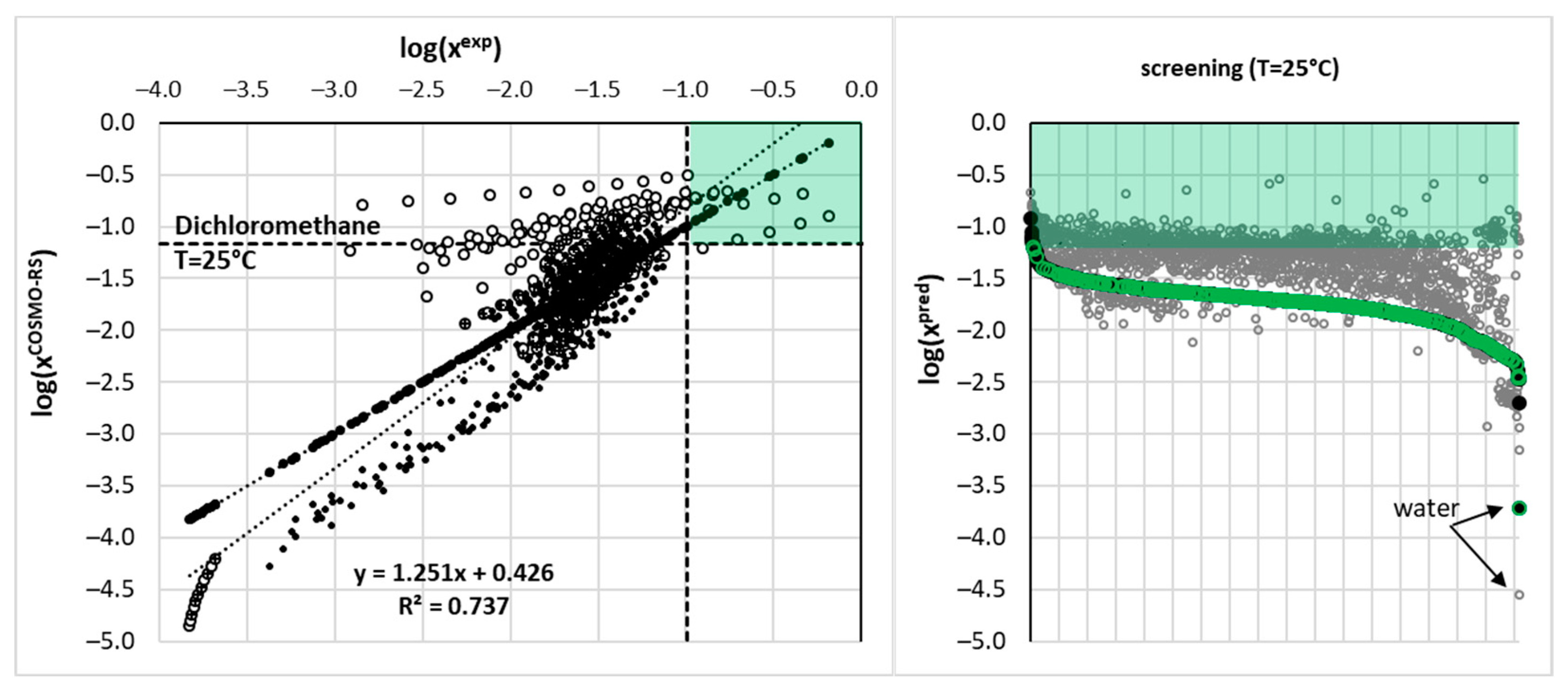
Figure 8.
The results of optimization of the ΔCp value for solubility computations using the COSMO-RS approach.
Figure 8.
The results of optimization of the ΔCp value for solubility computations using the COSMO-RS approach.
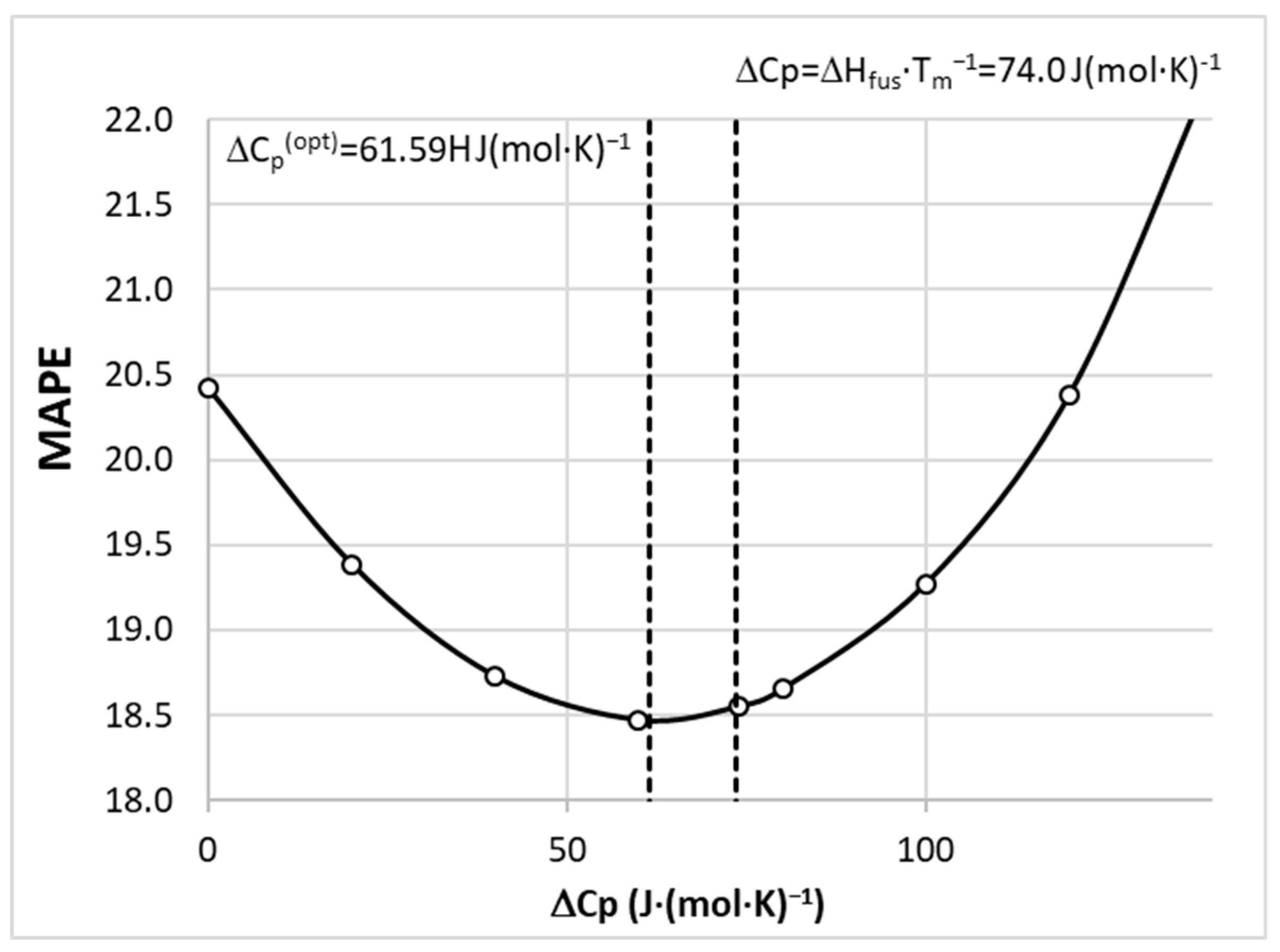

Table 1.
Collection of five top-ranked solvents most suited for edaravone. In parenthesis, values predicted by the COSMO-RS approach are given.
Table 1.
Collection of five top-ranked solvents most suited for edaravone. In parenthesis, values predicted by the COSMO-RS approach are given.
| solvent | CAS | log(xEest) | EI(PCOP=0) |
| enflurane /[13838-16-9] |
 |
–1.20±0.42 /(–1.29) |
0.47 |
| DMSO /[67-68-5] |
 |
–1.22±0.20 /(–1.28) |
0.26 |
| isoflurane /[26675-46-7] |
 |
–1.29±0.46 /(–1.05) |
0.56 |
| NMP /[872-50-4] |
 |
–1.40±0.09 /(–0.92) |
0.97 |
| 2-ethenoxyethanol /[764-48-7] |
 |
–1.41±0.09 /(–1.35) |
0.97 |
Disclaimer/Publisher’s Note: The statements, opinions and data contained in all publications are solely those of the individual author(s) and contributor(s) and not of MDPI and/or the editor(s). MDPI and/or the editor(s) disclaim responsibility for any injury to people or property resulting from any ideas, methods, instructions or products referred to in the content. |
© 2023 by the authors. Licensee MDPI, Basel, Switzerland. This article is an open access article distributed under the terms and conditions of the Creative Commons Attribution (CC BY) license (https://creativecommons.org/licenses/by/4.0/).
Copyright: This open access article is published under a Creative Commons CC BY 4.0 license, which permit the free download, distribution, and reuse, provided that the author and preprint are cited in any reuse.


