Submitted:
18 August 2023
Posted:
22 August 2023
You are already at the latest version
Abstract
This paper studies the finite-time synchronization problem of fractional-order stochastic memristive bidirectional associative memory neural networks (MBAMNNs) with discontinuous jumps. A novel criterion for finite-time synchronization is obtained by utilizing the properties of quadratic fractional-order Gronwall inequality with time delay and the comparison principle. This criterion provides a new approach to analyze the finite-time synchronization problem of neural networks with stochasticity. Finally, numerical simulations are provided to demonstrate the effectiveness and superiority of the obtained results.
Keywords:
stochastic
; fractional-order
; memristive BAM neural networks
; finite-time synchronization
; quadratic gronwall inequality
1. Introduction
Artificial intelligence has been an active field of research, and neural networks have emerged as a prominent branch due to their intelligence characteristics and potential for real-world applications. Neural networks have revolutionized the field of artificial intelligence by enabling computers to process and analyze large volumes of complex data with remarkable accuracy. These models are based on the structure and processes of the brain, where neurons are interconnected and communicated by using electrical signals. Neural networks are characterized by their remarkable ability to learn from data and improve their performance over time, without being explicitly programmed. Neural networks have evolved over time, with various models developed to address different types of problems. For example Cohen-Grossberg neural networks [1], Hopfield neural networks [2] and cellular neural networks [3].
Kosko’s bidirectional associative memory neural networks (BAMNNs) are noteworthy extension of the traditional single-layer neural networks [4]. The BAMNNs consist of two layers of neurons that are not interconnected within their own layer. In contrast, the neurons in different layers are fully connected, allowing for bidirectional information flow between the two layers. This unique structure enables the BAMNNs to function as both input and output layers, providing powerful information storage and associative memory capabilities. In signal processing, the BAMNNs can be used to filter signals or extract features, while in pattern recognition, it can classify images or recognize speech. In optimization, the BAMNNs can be used to identify the optimal solution, while in automatic control, it can be used to regulate or stabilize a system. The progress of artificial intelligence and the evolution of neural networks have created novel opportunities to tackle intricate issues in diverse domains. In summary, these advancements have paved the way for innovative problem-solving approaches that were previously unattainable. The BAMNNs’ unique architecture and capabilities make its a powerful tool for engineering applications, and its is anticipated that this technology will maintain its importance in future research and development, and continue to make substantial contributions to various fields.
Due to the restriction of network size and synaptic elements, the functions of artificial neural networks are greatly limited. If common connection weights and the self-feedback connection weights of BAMNNs are established by memristor [5], then its model can be built in a circuit. Memristor [6,7] is a circuit element in electronic circuit theory that behaves nonlinearly and has two terminals. Its unique feature has led to its widespread use and potential application in a variety of fields, including artificial intelligence, data storage, and neuromorphic computing. Adding memristor to neural networks makes it possible for artificial neural networks to simulate human brain on the circuit, which makes the research on memristor neural networks more meaningful. Therefore, the resistance in the traditional neural networks is replaced by memristor, and the BAMNNs based on memristor is formed (MBAMNNs). Compared with traditional neural networks, Memristor neural networks have stronger learning and associative memory abilities, allowing for more efficient processing and storage of information, thereby improving the efficiency and accuracy of artificial intelligence. Additionally, due to the nonlinear characteristics of memristors and their applications in circuits, Memristor neural networks also have lower energy consumption and higher speed. Therefore, the development of Memristor neural networks have broad application prospects in the field of artificial intelligence.
However, due to the limitation of amplifier conversion speed, the phenomenon of time delay in neural network systems is inevitable. Research indicates that the presence of time delay is a significant factor contributing to complex dynamic behaviors such as system instability and chaos [8]. To enhance the versatility and efficiency of the BAMNNs, Ding and Huang [9] developed a novel BAMNNs model in 2006. The focus of their investigation was on analyzing the global exponential stability of the equilibrium point and studying its characteristics in this model. The time delay BAMNNs has been advanced by its positive impact on its development [10,11,12,13].
Fractional calculus extends the traditional differentiation and integration operations to non-integer orders [14], and has been introduced into neural networks to capture the characteristics of memory and inheritance [15,16,17]. The emergence of fractional-order calculus has spurred the development of neural networks [6,7,18,19], which have found applications in diverse areas, including signal detection, fault diagnosis, optimization analysis, associative memory, and risk assessment. The fractional-order memristive neural networks (FMNN) are the specific type of fractional-order neural networks, which have been widely studied for their stability properties. For instance, scholars have investigated the asymptotic stability of FMNNs with delay using Caputo fractional differentiation and Filippov solution properties [20], and also have investigated the asymptotic stability of FMNNs with delay by leveraging the properties of Filippov solutions and Leibniz theorem [21].
As one of the significant research directions in the nonlinear systems field, synchronization includes quasi-consistent synchronization [22], projective synchronization [23], full synchronization [24], Mittag-Leffler synchronization [25], global synchronization [26] and many other types. And it is widely used in cryptography [27], image encryption [28], secure communication [29]. In engineering applications, people want to realize synchronization as soon as possible, so the concept of finite time synchronization is proposed. Due to its ability to achieve faster convergence speed in network systems, finite-time synchronization has become a crucial aspect in developing effective control strategies for realizing system stability or synchronization [30,31].
This paper addresses the challenge of achieving finite-time synchronization. The definition of finite-time synchronization used in this article is that the synchronization error be kept within a certain range for a limited time interval. However, dealing with the time delay term in this context is challenging. Previous studies have utilized the Hölder inequality [32] and the generalized Gronwall inequality [33,34] to address the finite-time synchronization problem of fractional-order time delay neural networks, providing valuable insights into the problem. However, this paper proposes a new criterion based on the quadratic fractional-order Gronwall inequality with time delay and comparison principle, offering a fresh perspective on the problem.
This paper presents significant contributions towards the study of finite-time synchronization in fractional-order stochastic MBAMNNs with time delay. The key contributions are as follows:
(1) We improved Lemma 2 in [34] by deriving a quadratic fractional-order Gronwall inequality with time delay, which is a crucial tool for analyzing the finite-time synchronization problem in stochastic neural networks.
(2) A novel criterion for achieving finite-time synchronization is proposed, which allows for the computation of the required synchronization time T. This criterion provides a new approach to analyze finite-time synchronization and has the potential to be widely applicable in the field of neural networks research. The paper is structured as follows: Section 2 introduces relevant concepts and presents the neural networks model used in this study. Section 3 proposes a novel quadratic fractional-order Gronwall inequality that takes into account time delay. This inequality is useful for studying the finite-time synchronization problem in fractional-order stochastic MBAMNNs with time delay, and by utilizing differential inclusion and set-valued mapping theory, a new criterion for determining the required time T for finite-time synchronization is derived. Section 4 provides a numerical example that demonstrates the effectiveness of the proposed results. Finally, suggestions for future research are presented.
2. Preliminaries and model
This section provides an overview of the necessary preliminaries related to fractional-order derivatives and the model of fractional-order stochastic MBAMNNs. We begin by introducing the fundamental concepts related to fractional-order derivatives and then move on to describe the fractional-order stochastic MBAMNNs model. And the definition of finite-time synchronization is provided.
2.1. Preliminaries
Notations: The norm and absolute value of vectors and matrices are defined as follows. Let N and denote the sets of positive integers and real numbers, respectively.
The norm of a vector is given by . Similarly, the norm of a vector is defined as .The induced norm of a matrix is denoted by .The absolute value of a vector is defined as .
Following that, we provide a review and introduction of several definitions and lemmas related to fractional calculus.
Definition 1.
Especially, for
Definition 2.
[35] Suppose , where ι is a positive integer. The Caputo derivative of order α of the function can be expressed as:
where
For the convenience, we use to represent
Lemma 1.
2.2. Model
We investigate a kind of fractional-order differential equations that capture the dynamics of fractional-order stochastic MBAMNNs with time delays. These equations are viewed as the driving system (1), which models the interactions between neurons in MBAMNNs and accounts for the influence of discontinuous jumps and time delays. Through examining the stability and analytical solutions of these equations, this study aims to enhance the comprehension of the behavior of MBAMNNs, ultimately leading to more comprehensive analysis for practical applications of this model.
where
In this system, the positive parameters and represent the rates of neuron self-inhibition, while and denote the state variables of the -th and -th neuron, respectively. The activation functions without time delay are denoted by and , and those with time delay are denoted by and . The neural connection memristive weights matrices are represented by , , , and . Stochastic terms representing Brownian motion are denoted by and . The constant input vectors are represented by and . The time delay parameters and satisfy and , where is a constant.
The initial conditions of fractional-order stochastic MBAMNNs (1) are given by , where and . Here, and are continuous functions on and .
Then, the corresponding system of drive system (1) is gived by
The initial conditions of the corresponding system (2) are ; and are the following controllers:
where and are both positive numbers called the control gain.
Then we obtain synchronization error is And denote
Definition 3.
Remark 1.
The next section will apply Lemma 1, which provides a quadratic fractional Gronwall inequality with time delay. This inequality is used to analyze the behavior of the MBAMNNs system.
3. Main results
This section presents a novel approach to obtain the evaluation function by improving quadratic fractional Gronwall inequality with time delay. We then utilize Theorem 1 to convert this inequality into a format that is consistent with Lemma 2, enabling us to derive a synchronization criterion for the drive system (1) and corresponding system (2) in finite time. Specifically, the application of Lemma 2 leads to the novel criterion for finite-time synchronization.
Quadratic fractional Gronwall inequality with time delay is given below.
Lemma 2.
Let and , , , and be continuous functions that are nonnegative and defined on . Let be a nonnegative continuous function defined on and suppose
Assume and are nondecreasing on , is nondecreasing on and
(1) If then
(2) If then
where and they are all constants.
Proof
(Proof). Define a function by
As shown in Equation (3), we get
When and the function , then
From Lemma 1, we obtain
Assume are nondecreasing on , is nondecreasing on and .
(1) If , then
(2) If , similar to case (1), we obtain
For , we get
Then, by utilizing Lemma 1 and inequality (5), we arrive at
By using (4), we have
Similarly, assume are nondecreasing on , is nondecreasing on and .
(1) If , then
(2) If , then
Based on the above analysis, from Lemma 2 and when and are non-decreasing functions for , is a non-decreasing function for with we get the following results.
(1) If then
(2) If then
□
Theorem 1.
Assume and non-negative continuous functions , , , , and defined on . Let be a non-negative continuous function defined on and suppose
Assume and are nondecreasing functions on , and is a nondecreasing function on with .
(1) If then
(2) If then
where and such that and
Proof
(Proof). By using the Hölder inequality, it follows that
Let then from Lemma 2 we obtain
The proof is completed. □
To analyze the solutions of the discontinuous systems represented by equations (1) and (2), Filippov regularization is used. This involves transforming the equations into differential inclusions and set-valued maps.
The drive system represented by equation (1) can be expressed in terms of a differential inclusion, which is a powerful tool in the theory of differential inclusions. By using this approach, we can study the behavior of the system even when it experiences discontinuities or impulses.
Overall, Filippov regularization allows us to analyze the solutions of discontinuous systems like Equations (1) and (2) in a rigorous and systematic way, providing insights into their behavior and enabling us to make informed decisions about their design and operation.
According to the definition of set-valued maps, we obtain
where the switching jumps are positive contants, , , , , , , , , , , and are all contant numbers. , , , , , are all compact, closed and convex.
Let
By modifying the drive system (1), we can achieve
Similarly, let
by employing the similar method, we can modify the corresponding system (2) as follows:
Assumption A1.
Let function satisfy the Lipschitz condition, there exist positive constants such that
where are positive Lipschitz constants and assume functions and satisfy this condition equally.
Assumption A2.
Lemma 3.
The synchronization error system, by Assumption A1 and Lemma 3, can be expressed as:
where denote and
For the sake of convenience, we can express inequality (8) as
where and
Remark 2.
To ensure that , we can simply find an evaluation function that satisfies with This will guarantee that remains below ϵ, while it also will ensure that is never less than
Lemma 4.
Theorem 2.
Assume Assumption A1, Assumption A2 and Remark 2 hold and the following conditions are satisfied.
(1) If then
(2) If then
where and ().
Proof
(Proof).
By Definition 1, for , we can obtain the following integral inequalities:
Assuming we can square both sides to obtain . By using Lemma 4, we can then rewrite the expression as follows
From Lemma 2, we define the following functions: , , , and . The initial value and . It is easy to see that all of these functions are non-negative and continuous. Additionally, and are non-decreasing on , is non-decreasing on and .
By using Lemma 2, we can obtain the following results.
(1) If then
(2) If then
where
So when , Remark 2 indicates that the evaluation function can be determined as follows.
(1) If then
(2) If then
4. Numerical examples
Compared to conventional neural networks, neural networks incorporating stochasticity possess greater adaptability and robustness in achieving finite-time synchronization. This is because stochasticity can increase the complexity of the system, endowing it with enhanced fault-tolerance and adaptability, thus facilitating more efficient adaptation to diverse environments and application scenarios. Moreover, neural networks with stochasticity exhibit advantageous characteristics in handling nonlinear and complex problems. In practical applications, the parameters and states of the neural network systems are often uncertain, owing to the presence of uncertainty. Stochasticity can more effectively model such uncertainty and bolster the reliability of the neural network systems, thereby elevating its performance in practical applications. Therefore, investigating neural networks with stochasticity may contribute to enhancing the application capabilities and performance of neural networks.
We illustrate the practical application of Theorem 2 in achieving finite-time synchronization between the systems (1) and (2) through a numerical example. By showing this example, we can validate the effectiveness of the proposed synchronization method. Specifically, the example involves simulating the behavior of the systems with varying initial conditions, and analyzing the resulting trajectories. The insights gained from this example are used to serve as evidence to show the practical relevance of the finite-time synchronization approach presented in this paper.
Example
Consider the fractional-order stochastic MBAMNNs with time delay
where
Let
Then, assume and in corresponding system (2).
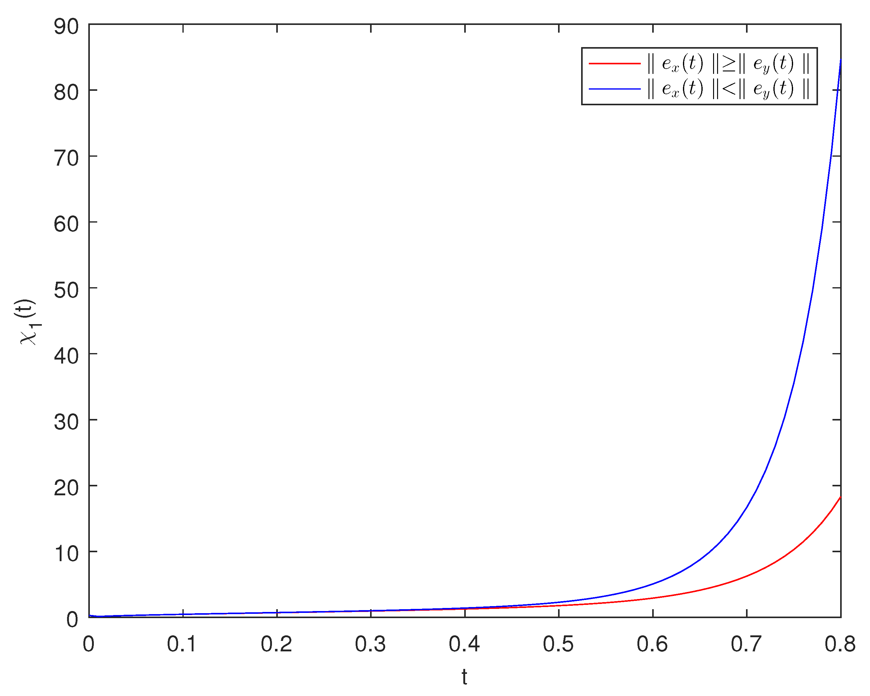
Let such that It is easy to calculate that and By analyzing Figure 1 and Figure 2, we can obtain the error components and of systems (1) and (2) when and . By using Figure 3 and Figure 4, we can calculate the error and square of error of systems (1) and (2). Finally, based on Figure 5 and Theorem 2, we can determine the finite-time synchronization time .
5. Conclusions
We have enhanced the fractional-order Gronwall inequality for studying finite-time synchronization in fractional-order stochastic MBAMNNs systems, based on the work originally proposed in [34]. Then we presented an illustrative example to show the effectiveness of our proposed approach. However, it should be noted that we have only analyzed the finite-time synchronization of continuous neural network systems, and have not provided a detailed description of discontinuous neural networks with impulses. Hence, we will investigate the dynamic behaviors of fractional-order neural networks with impulses in the future.
Author Contributions
All authors contributed equally and significantly in writing this article. All authors read and approved the final manuscript.
Funding
This research was funded by Shandong Provincial Natural Science Foundation under grant ZR2020MA006 and the Introduction and Cultivation Project of Young and Innovative Talents in Universities of Shandong Province.
Institutional Review Board Statement
Not applicable.
Informed Consent Statement
Not applicable.
Data Availability Statement
Not applicable.
Acknowledgments
We would like to express our thanks to the anonymous referees and the editor for their constructive comments and suggestions, which greatly improved this article.
Conflicts of Interest
The authors declare no conflict of interest.
References
- Cohen, M.A.; Grossberg, S. Absolute stability of global pattern formation and parallel memory storage by competitive neural networks. IEEE Trans. Syst. Man Cybernet. 1983, SMC-13 (5), 815–826. [Google Scholar] [CrossRef]
- Hopfield, J.J. Neural networks and physical systems with emergent collective computational abilities, Proc. Natl. Acad. Sci. USA. 1982, 79(8), 2554–2558. [Google Scholar] [CrossRef] [PubMed]
- Chua, L.O.; Yang, L. Cellular neural networks: theory, IEEE Trans. Circuit. Syst. 1988, 35(10), 1257–1272. [Google Scholar]
- Kosko, B. Bidirectional associative memories, IEEE Trans. Syst. Man Cybernet. 1988, 18(1), 49–60. [Google Scholar] [CrossRef]
- Xiao, J.; Zhong, S.; Li, Y.; et al. Finite-time Mittag–Leffler synchronization of fractional-order memristive BAM neural networks with time delays. Neurocomputing 2017, 219, 431–439. [Google Scholar] [CrossRef]
- Zhang, W.; Zhang, H.; Cao, J.; et al. Synchronization in uncertain fractional-order memristive complex-valued neural networks with multiple time delays. Neural Netw. 2019, 110, 186–198. [Google Scholar] [CrossRef]
- Zhang, W.; Zhang, H.; Cao, J.; et al. Synchronization of delayed fractional-order complex-valued neural networks with leakage delay, Phys. A. 2020, 556, 124710. [Google Scholar]
- Marcus, C.M.; Westervelt, R.M. Stability of analog neural networks with delay, Phys. Rev. A. 1989, 39(1), 347. [Google Scholar] [CrossRef]
- Ding, K.E.; Huang, N.J. Global robust exponential stability of interval general BAM neural network with delays, Neural Process. Lett. 2006, 23(2), 171–182. [Google Scholar]
- Zhang, Z.; Yang, Y.; Huang, Y. Global exponential stability of interval general BAM neural networks with reaction–diffusion terms and multiple time-varying delays. Neural Netw. 2011, 24, 457–465. [Google Scholar] [CrossRef]
- Wang, D.; Huang, L.; Tang, L. Dissipativity and synchronization of generalized BAM neural networks with multivariate discontinuous activations, IEEE Trans. Neural Netw. Learn. Syst. 2017, 29(8), 3815–3827. [Google Scholar]
- Xu, C.; Li, P.; Pang, Y. Global exponential stability for interval general bidirectional associative memory (BAM) neural networks with proportional delays, Math. Methods Appl. Sci. 2016, 39(18), 5720–5731. [Google Scholar] [CrossRef]
- Duan, L. Existence and global exponential stability of pseudo almost periodic solutions of a general delayed BAM neural networks, J. Syst. Sci. Complex. 2018, 31(2), 608–620. [Google Scholar] [CrossRef]
- Diethelm, K.; Ford, N.J. Analysis of fractional differential equations, J. Math. Anal. Appl. 2002, 265(2), 229–248. [Google Scholar] [CrossRef]
- Magin, R.L. Fractional calculus models of complex dynamics in biological tissues, Comput. Math. Appl. 2010, 59, 1585–1593. [Google Scholar]
- Li, L.; Wang, X.; Li, C.; et al. Exponential synchronizationlike criterion for state-dependent impulsive dynamical networks, IEEE Trans. Neural Netw. Learn. Syst. 2018, 30, 1025–1033. [Google Scholar] [CrossRef]
- Picozzi, S.; West, B.J. Fractional Langevin model of memory in financial markets, Phys. Rev. E. 2001, 66, 046118. [Google Scholar]
- Kaslik, E.; Sivasundaram, S. Nonlinear dynamics and chaos in fractional-order neural networks. Neural Netw. 2012, 32, 245–256. [Google Scholar] [CrossRef]
- Ding, D.; You, Z.; Hu, Y.; et al. Finite-time synchronization of delayed fractional-order quaternion-valued memristor-based neural networks, Int. J. Mod. Phys. B. 2021, 35(03), 2150032. [Google Scholar] [CrossRef]
- Chen, J.; Jiang, M. Stability of memristor-based fractional-order neural networks with mixed time-delay and impulsive, Neural Process. Lett. 2022, 1–22. [Google Scholar]
- Chen, J.; Chen, B.; Zeng, Z. Global asymptotic stability and adaptive ultimate Mittag–Leffler synchronization for a fractional-order complex-valued memristive neural networks with delays, IEEE Trans. Syst. Man Cybernet. 2018, 49(12), 2519–2535. [Google Scholar] [CrossRef]
- Yang, X.; Li, C.; Huang, T.; et al. Quasi-uniform synchronization of fractional-order memristor-based neural networks with delay. Neurocomputing 2017, 234, 205–215. [Google Scholar] [CrossRef]
- Yang, S.; Yu, J.; Hu, C.; et al. Quasi-projective synchronization of fractional-order complex-valued recurrent neural networks. Neural Netw. 2018, 104, 104–113. [Google Scholar] [CrossRef] [PubMed]
- Chen, L.; Wu, R.; Cao, J.; et al. Stability and synchronization of memristor-based fractional-order delayed neural networks. Neural Netw. 2015, 71, 37–44. [Google Scholar] [CrossRef] [PubMed]
- Chen, J.; Zeng, Z.; Jiang, P. Global Mittag-Leffler stability and synchronization of memristor-based fractional-order neural networks. Neural Netw. 2014, 51, 1–8. [Google Scholar] [CrossRef] [PubMed]
- Yang, X.; Li, C.; Huang, T.; et al. Synchronization of fractional-order memristor-based complex-valued neural networks with uncertain parameters and time delays. Chaos, Solitons Fractals. 2018, 110, 105–123. [Google Scholar] [CrossRef]
- Muthukumar, P.; Balasubramaniam, P. Feedback synchronization of the fractional order reverse butterfly-shaped chaotic system and its application to digital cryptography. Nonlinear Dyn. 2013, 73, 1169–1181. [Google Scholar] [CrossRef]
- Wen, S.; Zeng, Z.; Huang, T.; et al. Lag synchronization of switched neural networks via neural activation function and applications in image encryption, IEEE Trans. Neural Netw. Learn. Syst. 2015, 7, 1493–1502. [Google Scholar] [CrossRef]
- Alimi, A.M.; Aouiti, C.; Assali, E.A. Finite-time and fixed-time synchronization of a class of inertial neural networks with multi-proportional delays and its application to secure communication. Neurocomputing. 2019, 332, 29–43. [Google Scholar] [CrossRef]
- Ni, J.; Liu, L.; Liu, C.; et al. Fast fixed-time nonsingular terminal sliding mode control and its application to chaos suppression in power system. IEEE Trans. Circuits Syst. II-Express Briefs. 2017, 64, 151–155. [Google Scholar] [CrossRef]
- Zhang, D.; Cheng, J.; Cao, J.; et al. Finite-time synchronization control for semi-Markov jump neural networks with mode-dependent stochastic parametric uncertainties, Appl. Math. Comput. 2019, 344, 230–242. [Google Scholar]
- Pratap, A.; Raja, R.; Cao, J.; Rajchakit, G.; Alsaadi, F.E.; et al. Further synchronization in finite time analysis for time-varying delayed fractional order memristive competitive neural networks with leakage delay. Neurocomputing. 2018, 317, 110–126. [Google Scholar]
- Ye, H.; Gao, J.; Ding, Y. A generalized Gronwall inequality and its application to a fractional differential equation, J. Math. Anal. Appl. 2007, 328(2), 1075–1081. [Google Scholar] [CrossRef]
- Du, F.; Lu, J.G. New criterion for finite-time synchronization of fractional-order memristor-based neural networks with time delay, Appl. Math. Comput. 2021, 389, 125616. [Google Scholar]
- Kilbas, A.A.; Marzan, S.A. Nonlinear differential equations with the Caputo fractional derivative in the space of continuously differentiable functions, Differ. Equ. 2005, 41(1), 84–89. [Google Scholar]
- Bainov, D.D.; Simeonov, P.S. Integral Inequalities and Applications. Springer: New York, NY, USA, 1992. [Google Scholar]
- Chen, J.; Zeng, Z.; Jiang, P. Global Mittag-Leffler stability and synchronization of memristor-based fractional-order neural networks. Neural Netw. 2014, 51, 1–8. [Google Scholar] [CrossRef]
- Rao, R.; Pu, Z. Stability analysis for impulsive stochastic fuzzy p-laplace dynamic equations under neumann or dirichlet boundary condition, Bound. Value Probl. 2013, 2013, 133. [Google Scholar] [CrossRef]
Figure 1.
The errors and are computed for and with .
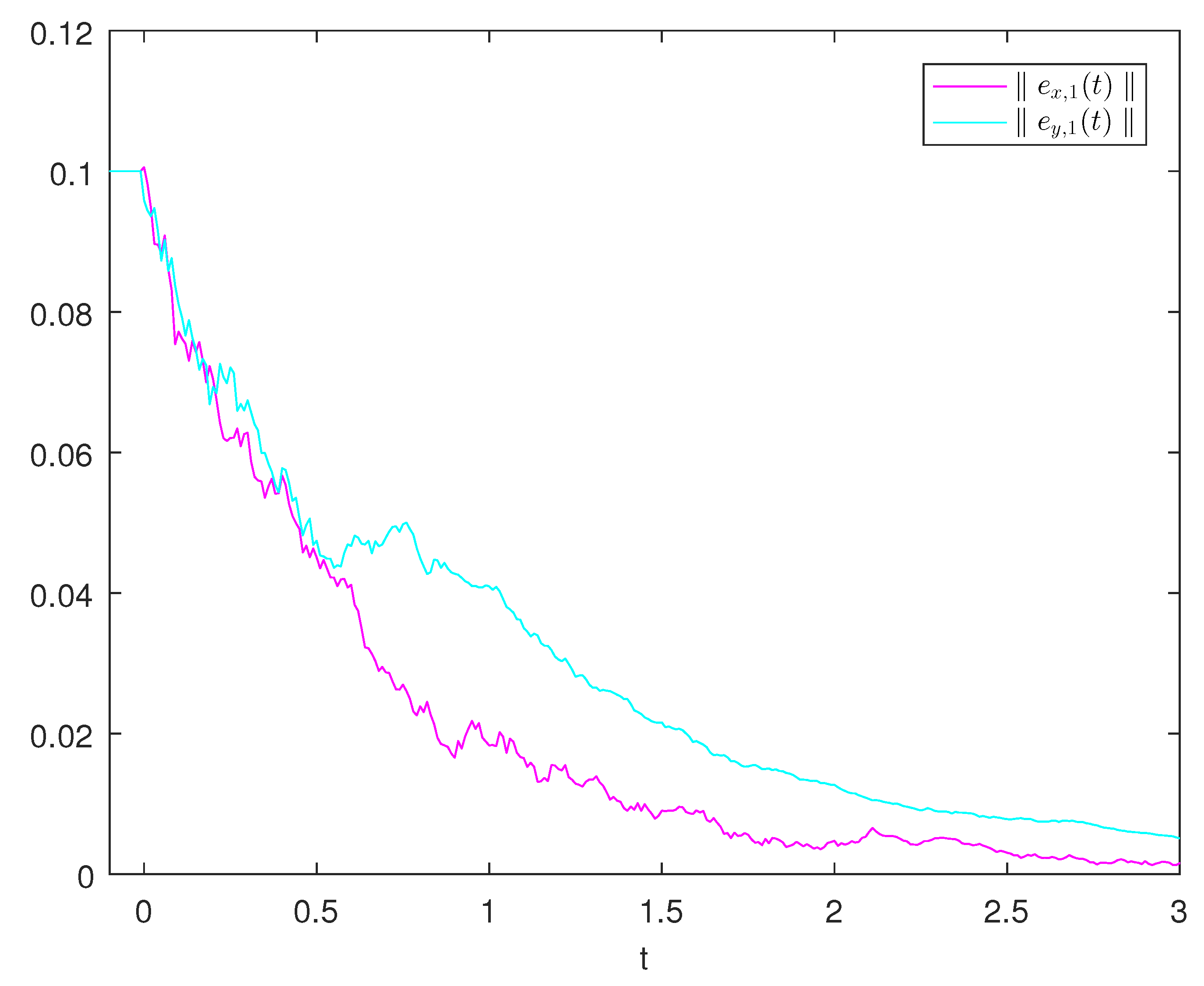
Figure 2.
The errors and are computed for and with .
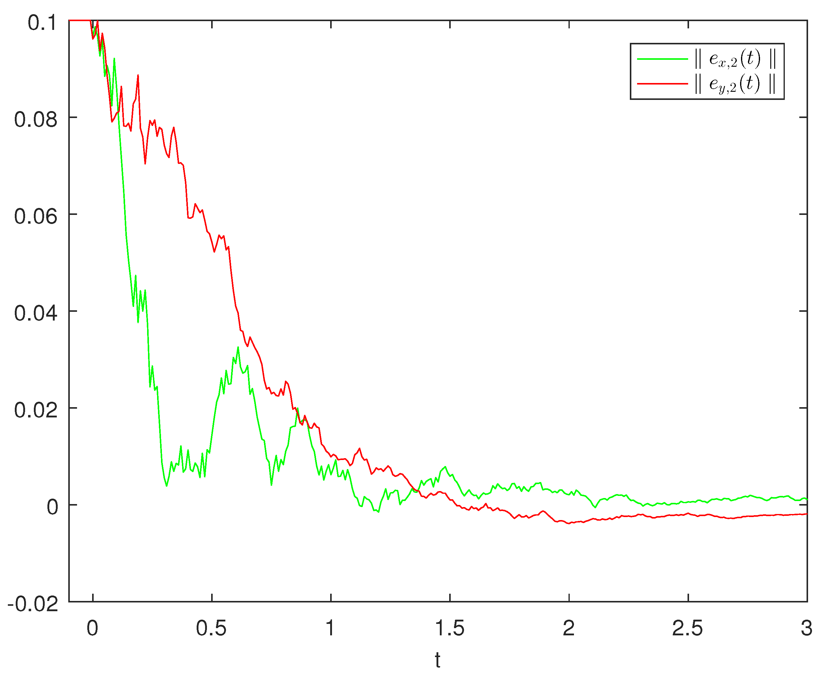
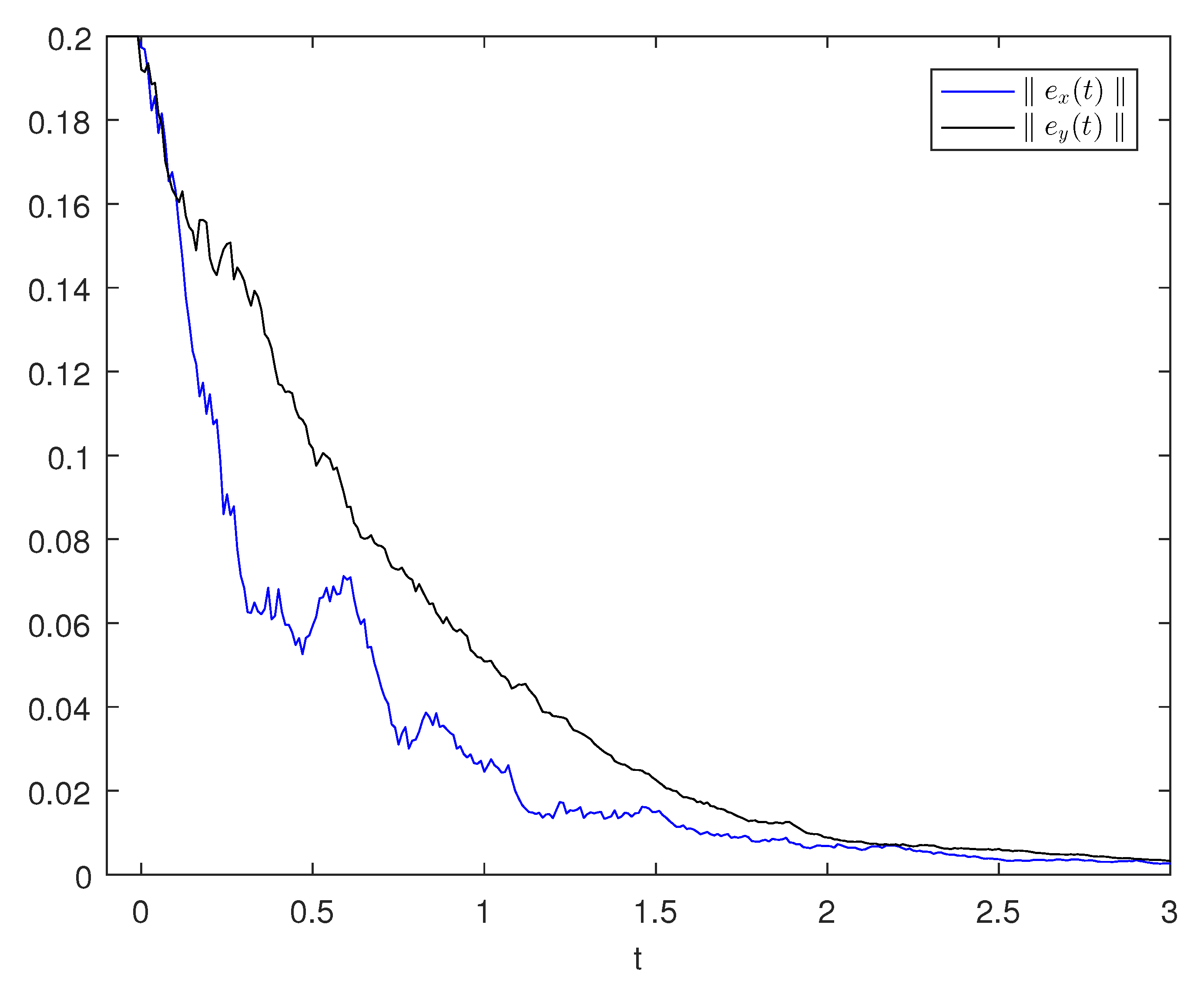
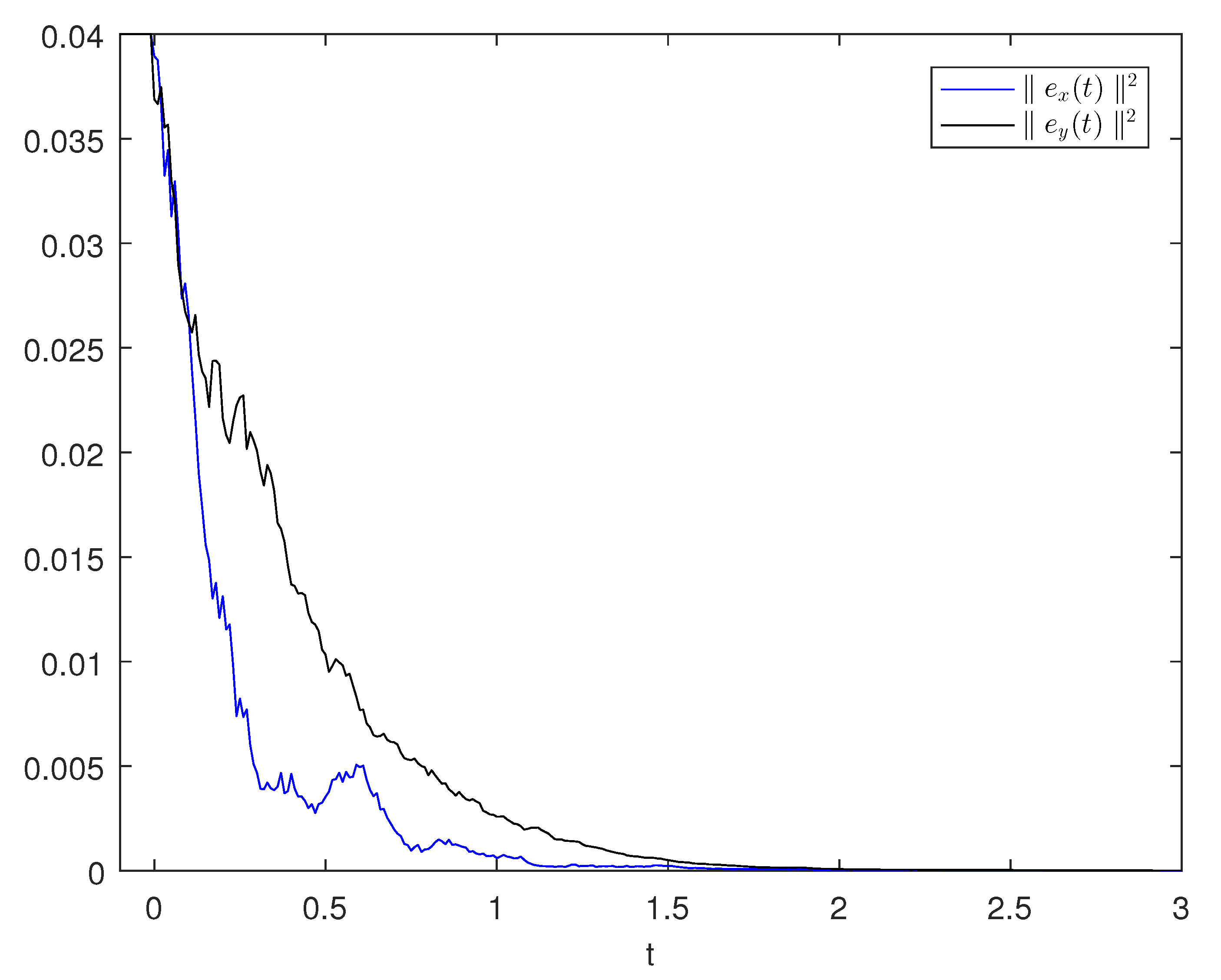
Figure 5.
The evaluation function with .
Disclaimer/Publisher’s Note: The statements, opinions and data contained in all publications are solely those of the individual author(s) and contributor(s) and not of MDPI and/or the editor(s). MDPI and/or the editor(s) disclaim responsibility for any injury to people or property resulting from any ideas, methods, instructions or products referred to in the content. |
© 2023 by the authors. Licensee MDPI, Basel, Switzerland. This article is an open access article distributed under the terms and conditions of the Creative Commons Attribution (CC BY) license (http://creativecommons.org/licenses/by/4.0/).
Copyright: This open access article is published under a Creative Commons CC BY 4.0 license, which permit the free download, distribution, and reuse, provided that the author and preprint are cited in any reuse.


