
Submitted:
20 August 2023
Posted:
21 August 2023
You are already at the latest version
Abstract
We present a near real-time solution for 3D reconstruction from aerial images captured by consumer UAVs. Our core idea is to simplify the multi-view stereo problem into a series of two-view stereo matching problems. Our method applies to UAVs equipped with only one camera and does not require special stereo-capturing setups. We found that the neighboring two video frames taken by UAVs flying at a mid-to-high cruising altitude can be approximated as left and right views from a virtual stereo camera. Leveraging GPU-accelerated real-time stereo estimation, efficient PnP correspondence solving algorithms and extended Kalman filter, our system simultaneously predicts scene geometry and camera position/orientation from the virtual stereo cameras. Also, this method allows user selection of varying baseline lengths, which provides more flexibility given the trade-off between camera resolution, effective measuring distance, flight altitude, and mapping accuracy. Our method outputs dense point clouds at a constant speed of 25 frames per second and is validated on a variety of real-world datasets with satisfactory results.
Keywords:
3D Reconstruction
; Unmanned Aerial Vehicles
; Real-time Systems
1. Introduction
Recent advances in chipmaking and imaging sensor technologies enabled micro unmanned aerial vehicles (UAV) to reduce cost and quickly progress into consumer markets. Micro UAVs are widely used in agriculture, construction, transportation, and film-making because of their exceptional stability, mobility, and flexibility. Specifically, aerial remote sensing provides a rapid, inexpensive, and highly automated approach to producing 3D digital assets for easy measurement, inspection, planning, and management. Currently, large-scale terrestrial scans are typically done by ground-based LiDAR systems. However, such systems are bulky, expensive, power-intensive, and often unable to provide dense textured mesh. It is more desirable to enable real-time high-resolution mapping capabilities for consumer-level camera drones. Compared to terrestrial LiDARs, consumer UAVs capture high-quality data in less time and at a lower overall cost. Also, the operational complexity is much less for drones compared to terrestrial LiDAR workflows. The redundancy of overlapping images, together with georeferencing and auto-alignment enforced by photogrammetry algorithms, translates to high accuracy outputs even in non-ideal operational or imaging conditions.
However, current photogrammetry pipelines usually take hours to days to fully process captured imagery data, which greatly limits their capability for real-time data acquisition. Such ability is essential in scenarios such as onsite scan and inspection, emergency response and planning, etc. An ideal scanning pipeline should be able to map the scene in real time as the drone travels along the flight path, and gives inspectors the ability to examine the partial scan even before the flight mission is finished. Currently, it is difficult to achieve such goals using photogrammetry approaches, for a few reasons. Firstly, photogrammetry approaches typically require global optimization for camera pose estimation, dense multi-view stereo matching, meshing and texture mapping. So, at the framework level it prevents online real-time mapping in an incremental manner. Some algorithms first loads all feature points into memory and begins from the initial image pairs then incrementally extends the scene by registering new images and new 3D points. Our method is along the lines of performing incremental 3D reconstructions. However, our method still has subtle differences from the aforementioned approaches. Our method performs feature extraction, verification, camera pose estimation/refinement and dense stereo all at the same time on a frame-by-frame basis, whereas other approaches still separates the whole process into stages. For example, in most competitor approaches the dense multi-view stereo matching step cannot begin without the camera pose estimation (or SfM/sparse reconstruction) process completed for all images. In such cases, although the camera pose estimation or sparse point cloud reconstruction step is performed incrementally, the whole pipeline still requires the entire dataset as input, thus not applicable for online or real-time reconstruction. Secondly, for most of the prior work the structure from motion (SfM) and multi-view stereo (MVS) components used in their pipelines are typically computationally intensive and time-consuming. SfM algorithms typically densely scan the input images and extract feature points in order to find correspondences between these images in different views. Thirdly, a few failures or mismatches of images may break the entire photogrammetry pipeline. Imaging issues such as reflection, lack of texture, strong lighting, and moving objects may also result in poorly reconstructed scenes.
To tackle this problem, we propose an alternative approach. At the core of our design is to use high-efficiency algorithms with the lowest computational cost at each and every step of the pipeline. Therefore, we choose to use Harris corner [1] instead of SIFT [2] or SURF descriptors [3] for feature extraction. We adopt real-time Belief Propagation (BP) stereo matching on downsampled images instead of running large-scale full-resolution MVS matching. We also use the very fast EPnP [4] algorithm instead of performing Bundle Adjustment (BA) [5,6] as in many SfM pipelines. Finally, we employ EKF filter [7] to ensure reconstruction accuracy. The resulting system outputs an accurate dense point cloud in near real-time at a constant speed of 25 frames per second.
2. Related Work
Global vs. Local Stereo Matching Because of computing efficiency and accuracy constraints, for this work, we are only investigating stereo algorithms before the deep learning era. Deep learning algorithms have made tremendous progress in terms of both speed and accuracy for this task. However, such algorithms require special hardware and training data. Collecting the training data is very time-consuming and labor-intensive. In contrast, traditional stereo matching algorithms are bottom-up and unsupervised; and do not require any training data. Such algorithms are generally composed of the following stages: 1. cost computation; 2. cost aggregation, 3. cost optimization, and 4. disparity refinement. The main difference between local/semi-local [8,9,10,11] and global [12,13,14,15,16,17] algorithms are whether one can construct and optimize a global energy function. Typically local algorithms are based on computing windows and are sensitive to occlusion and homogeneous regions. Global methods are time-consuming but are much more accurate. This is done by incorporating smoothness terms and ensuring an optimal/sub-optimal solution via multiple iterations to reduce the global energy. In recent years, due to the rapid development of high-performance parallel computing hardware, it is possible to issue several thousands of threads at the same time to speed up the disparity calculation. By leveraging such massively parallel computing frameworks it is possible to perform global stereo matching in real-time.
vSLAM vs. SfM Visual SLAM [18,19,20,21,22] and SfM approaches [6,23,24,25] are both based on multiview geometry and both aiming at solving the camera motion/ scene geometry estimation problem. The main difference between the two methods is in time complexity requirements and practical applications. Typically SLAM is used in robotic applications focusing on using a single visual sensor with limited computing resources. Algorithms along this line generally use a very fast feature detector (e.g. LSD [22], ORB [19], FAST [26] etc.) and incorporate predictive/closed loop estimation frameworks to adjust the trajectory. Scene geometry estimation is a nice to-have feature but not mandatory. This is because most vSLAM applications are only aiming at getting the trajectory/pose graphs. In contrast, SfM algorithms are more geared towards reconstructing accurate 3D representations of the scene/objects. Therefore, SfM algorithms typically trade speed for accuracy, process data offline, and have a high demand for computing power [24]. SfM is often combined with multiview-stereo, surface reconstruction, and texture mapping steps to output the final mesh model. Such pipelines typically have very high requirements for imaging quality and are not very robust to real-world data (e.g. lens glare, motion/defocus blur, reflection/transparency, thin structures, etc.).
Aerial vs. Terrestrial Data Collection Using consumer drones for 3D reconstruction has many benefits compared to traditional ground-based survey practices. Firstly, drones can automatically fly in a pre-programmed pattern, collecting well-lit and occlusion-free images, while covering inaccessible or dangerous places with much lower risk (e.g. inspecting highway bridges without stopping traffic). Secondly, it only takes a fraction of the time and cost of ground-based surveys. Besides, the data collection process is reproducible, meaning that the drone could fly in the exact same pattern and collect data for comparison in the future. This is extremely helpful for tasks like inspecting structural cracks on highways/bridges/critical infrastructure, surveying coastline/sea floor/wetlands, or tracking of construction projects [27,28]. While consumer drones are great for aerial photogrammetry, there are a few drawbacks. Firstly, current onboard sensors and local obstacle avoidance systems are still not good enough for close-proximity flights, meaning that the drone could not collect enough parallax on vertical structures, limiting the accuracy of the final mesh when there is heavy occlusion. Secondly, LiDAR works on a variety of objects including specular/metallic surfaces and textureless regions with certain levels of see-through capability on transparent objects (e.g. cloud, rain, snow). On the contrary, photogrammetry algorithms operating on camera sensors will start to fail when reflective/textureless/transparent regions increase.
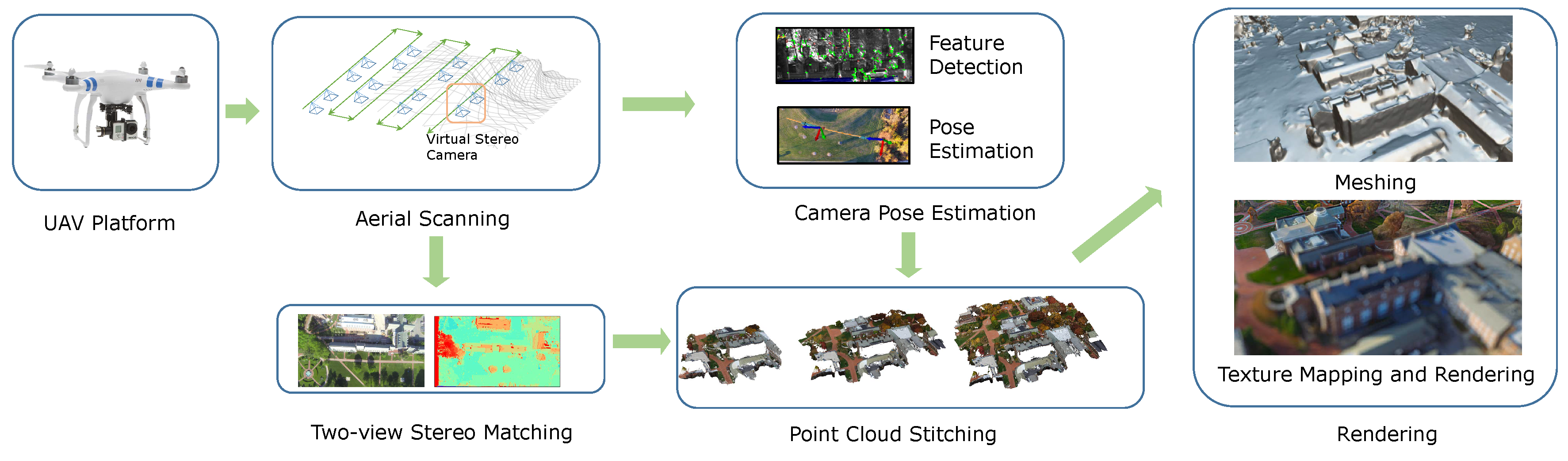
Figure 1.
The processing pipeline of our system. We decompose the multi-view reconstruction problem into pair-wise two-view stereo-matching problems. We perform fast camera pose estimation to stitch point clouds together and achieve near real-time speed at producing dense point clouds. Finally, we perform a meshing and texture mapping routine to obtain the final scanned model and visualize it in a web environment.
3. Methodology
3.1. Camera Calibration
Our goal is to generate scans of buildings and terrain with accurate measurements. Therefore, it is very important to map camera measurements to real-world coordinates. Since the GoPro camera we are using is wide-angle with severe distortion, we need to perform calibration to obtain the intrinsic parameters of the camera. Our method supposes that nearby frames captured by UAVs flying at high altitudes can be approximated as left and right views from a generic stereo camera system. Therefore, for camera calibration, we only recover the intrinsic parameters and ignore the calibration of extrinsic parameters. We also assume that the camera has only radial distortion and does not have any tangential distortion. More formally,
We use a planar checkerboard to calibrate the stereo camera [29]. In OpenCV [30], this process can be done by calling cvCalibrateCamera2(). Once we obtained the calibration parameters, we could rectify and undistort individual images so that a point projected in the left image will always have its correspondent point projection laying on the same scan line in the right image. This rectification process is done by calling cvInitUndistortMap() and cvRemap().
3.2. Depthmap Processing
Once the images are rectified, we seek to obtain depth maps representing 3D coordinates of real-world points in the camera coordination system. Our GoPro camera device is with 2.7K resolution recording at 60 frames per second. It is almost impossible to run traditional global stereo-matching methods on this resolution in real time. To address this problem, we choose to perform stereo matching on low-resolution image pairs first, and subsequently upsample the results with guidance from raw color images [31]. We use the GPU-based Belief Propagation [17] and Joint Bilateral Upsampling [32] in our implementation. We downsample the stereo image pairs to the resolution of 320 × 180 and seek to minimize the following energy function [17]:
Where is the message vector passed from a pixel to its neighbor. is the data term and is the smoothness term. After a given number of optimization iterations, the label d that minimizes is assigned to each pixel to form the disparity map. Next, we upsample the disparity map to obtain a high-resolution copy [32]:
The formula involves iterating over neighboring pixels in the downsampled depth map, represented by , within a filter window W centered around the pixel p in the high-resolution image. The upsampled depth value at position p is obtained by combining the downsampled depth values from neighboring pixels with spatial weight and range weight . The spatial weight measures the spatial distance between and , while the range weight captures the color similarity between the pixel values and at positions p and q in the high-resolution and input images, respectively. By combining spatial and range weights, the technique preserves edges and details during upsampling, reducing artifacts and noise in the output. This also combines appearance information with fine levels of details from the full-resolution image and spatial information from the downsampled disparity maps.
Once we have obtained the full resolution depth-map, suppose the baseline of the camera is B, and are lengths of the pixels on the horizontal and vertical axis, f is the focal length of the camera, is the 3D point coordinate in the camera coordinate system and is the 2D projection of the point on the imaging plane, we could get:
Therefore, we could obtain point clouds for all virtual stereo image pairs with respect to their own camera coordinate systems.
3.3. Pose Estimation and Refinement
Our approach supposes nearby frames taken from the aerial video with a fixed interval can be treated as a set of left-right image pairs taken by virtual stereo cameras with identical baselines. However, it is worth noting that this assumption only holds locally. If the time difference between the two frames are too much, then we cannot assume ideal stereo camera setup (exact same camera pose) and must re-estimate camera pose and orientation. In this section, we discuss how to recover orientations and poses for all virtual stereo cameras. Firstly, we need to introduce a feature descriptor to build correspondence between two camera frames. Instead of the commonly used SIFT [2]/ SURF [3] feature descriptor, we choose to use the very fast Harris corner detector for our application. Suppose the image is and we choose a patch with a small shift , the change of intensity could be formulated as [1]:
Where
A and B are first-order partial derivatives of the image, w is the gaussian window function to improve robustness to noises. is a matrix computed from the image derivatives. Harris corner is detected when the response R reaches the local maximum:
The Harris corner is related to the response from two directions and is thus invariant to rotation and translation. Also, the computation is relatively simple and could be performed in real-time. For a given threshold R, we choose a patch centered at every Harris corner, and compute correspondence between frame and , where t is the timestamp. The computation of correspondence will only be performed within the given search range. We use Squared Difference (ZSSD) to calculate the cost. Once the correspondences are obtained, we seek to obtain the rotation and translation matrices which describes the relative camera pose between time and . We adopt the very fast algorithm described in [4] for determining the position and orientation of the cameras given their calibrated intrinsics and a set of correspondences. At the core of this algorithm is to express 3D points as a weighted sum of 4 control points, reducing the computational complexity to . Suppose is the intrinsic matrix obtained from the previous section, are a set of Harris corners representing 3D points , we now have:
Where are projective parameters, are control points in the camera coordinate system. By solving this linear system, we could obtain the translation and rotation matrices which maps control point coordinates from real-world coordinate system to camera coordinate system:
Since the proposed system is completely based on visual information, it is possible that bad imaging conditions (e.g. textureless regions, reflective surface glares) would lead to inconsistency in feature matching between the stereo frames. Additionally, the presence of noise interference introduces considerable fluctuations in the computed results. Consequently, the utilization of filtering techniques becomes essential to obtain more reliable and smoother outcomes. Given the relatively smooth nature of the camera’s motion, without abrupt movements, we employ the Kalman filter based on a constant velocity model [7]. This choice is justified by its suitability for handling such motion characteristics and its potential to enhance the accuracy and robustness of the pose estimation results.
We begin by defining a 13-dimensional state vector as follows:
Where represents the 3D coordinates of the camera in the world coordinate system at time step . denotes the quaternion representation of the camera’s pose in the world coordinate system at time step . is the linear velocity vector of the camera with respect to the world coordinate system at time step . Finally, represents the angular velocity vector of the camera relative to the camera coordinate system at time step . These state variables constitute the essential elements for describing the camera’s position, orientation, linear velocity, and angular velocity at each time step in a 3D environment. The constant velocity model assumes that the camera motion is relatively smooth, without abrupt changes, and thus, it is suitable for accurately estimating the camera’s trajectory and poses in a continuous manner. Incorporating this model into our pose estimation framework will enable more reliable and accurate camera tracking results as our drone is programmed to move and capture images in constant velocity and altitude.
Let’s denote as the predicted state estimate at time step given the measurements up to time step k. It is computed using the function as follows:
The function transforms a rotation vector into a quaternion. and represent the noise sequences associated with linear velocity and angular velocity, respectively. They are considered to be zero-mean Gaussian random sequences with a covariance matrix . The measurements of satisfy a linear relationship, given by the measurement equation:
Where H is the measurement matrix
And represents the measurement noise at time step k, given by . This linear measurement equation enables the fusion of measurements with the predicted state to update and refine the state estimates using the Kalman filter. Therefore, we could derive the discrete-time predict and update equations on the camera poses. In the prediction stage, the predicted state and covariance estimate can be formulated as:
Where represents the predicted state estimate at time step k given all past measurements up to time step , and is obtained using the motion model . denotes the predicted state covariance matrix at time step k incorporating the uncertainty in the state estimate due to the motion model and control input . is the state transition matrix or Jacobian matrix of the motion model, while is the control matrix or Jacobian matrix of the motion model with respect to the control input . Finally, represents the e zero-mean noise added to the motion model at time step . In the update stage, we denote the near-optimal Kalman gain as: The updated state estimate can be calculated as: and the updated covariance estimate can be computed as:
Where represents the Kalman gain at time step k. The Kalman gain is a matrix used to determine the weight given to the current measurement and the predicted state estimate in the update process. It is calculated based on the predicted state covariance measurement matrix , measurement noise covariance matrix , and a Jacobian matrix of the measurement function to map the measurement noise covariance from the measurement space to the state space. denotes the predicted state covariance matrix at time step k given all past measurements up to time step . It represents the uncertainty in the state estimate. is the measurement matrix, which maps the state space into the measurement space. It defines how the state variables are related to the measurements obtained from the sensor. It is a constant matrix. represents the actual measurement obtained from the sensor at time step k. It is a vector that contains the measurements. denotes the predicted state estimate at time step k based on all past measurements up to time step . It is the expected value of the state variables given the previous measurements and the motion model. is a transformation matrix that is used to adjust the units or dimensions of the measurement noise covariance . It helps incorporate the measurement noise into the correct space. represents the measurement noise covariance matrix at time step k. It describes the uncertainty or noise present in the measurements obtained from the sensor. is the identity matrix, which has ones on the main diagonal and zeros elsewhere.
To this end, we could obtain camera poses for every virtually captured stereo pair obtained by the UAV. This also enables us to calculate real-time speed, traveled distances and turn angles of the UAV in real-world metrics without using any GPS information. Combined with the point clouds we obtained from Section 3.2, we could stitch the point cloud together into a combined point cloud of the captured scene along the flight trajectory. We use the EKF-filtered poses as initialization and use the CUDA accelerated Iterative Closest Point (ICP) [33] algorithm to fine-register all point clouds together. We run ICP on the point clouds calculated from low-resolution disparity maps using Equation 4. The final module which includes orientation/pose estimation and fine-registration is running at a constant speed of more than 100 Hz on a desktop equipped with a standalone GPU.
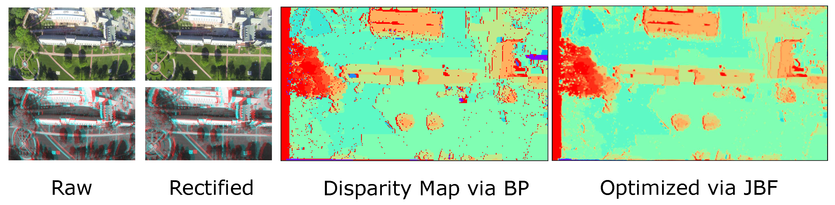
Figure 2.
Example output from our stereo matching module. The first and second columns show raw images and rectified images and corresponding analygraphs. The third row shows the disparity map generated by belief propagation stereo matching. The final row shows the optimized disparity map using joint bilateral upsampling. Note that small errors caused by BP are eliminated via JBF while all important edge details are preserved.
3.4. Meshing and Texture Mapping
To this end, we have shown an efficient approach to generate dense point cloud data. We also leverage Screened Poisson Surface Reconstruction [34] for mesh reconstruction and Large-Scale Texturing [35] for texture mapping.
Screened Poisson Surface Reconstruction aims to reconstruct a smooth surface, denoted as S, from an unorganized point cloud, denoted as P, with N points in . The goal is to find a scalar field over 3D space such that it satisfies the Poisson equation with a guidance function :
Where is the Laplacian operator. The guidance function is derived from the point cloud P and helps to direct the reconstruction process. To ensure a stable and smooth reconstruction, Screened Poisson Surface Reconstruction introduces a screening function that acts as a spatially varying weight. The screened Poisson equation is given by:
The screening function assigns higher weights to points near the surface and lower weights to points further away. This effectively suppresses the influence of noisy or distant points, resulting in a more robust and accurate reconstruction. The reconstructed surface S can be obtained by applying the marching cubes algorithm to the level set of the scalar field , where the level set defines the boundary of the surface. The marching cubes algorithm generates a triangular mesh that represents the reconstructed surface S. By incorporating the screening function into the Poisson equation, Screened Poisson Surface Reconstruction achieves a high-quality and smooth surface representation that respects the input point cloud while mitigating artifacts and irregularities.
Once we obtained the mesh, raw images and projection matrices, we can proceed with texture mapping. We could first start with image Projection. For each vertex in the 3D reconstruction, the corresponding 2D UV coordinates are computed by projecting onto the camera images. This projection is given by:
Where is the camera intrinsic matrix, is the camera projection matrix, and is the 3D vertex. Next we create the UV map. Using the computed UV coordinates, a UV map is created for each camera image. The UV map is a 2D representation of the camera image where each pixel corresponds to a 3D point on the reconstructed surface. To assign color information to the 3D reconstruction, we need to perform texture sampling. For each vertex , the corresponding color value is obtained by sampling the UV map at the UV coordinates . This process is given by:
Where Sample represents the sampling function. Finally, to handle occlusions and seams, we need to perform texture fusion. The color information from multiple camera images is fused together to obtain the final texture value at each vertex in the 3D reconstruction. This is done using a weighted averaging scheme:
Where N is the number of cameras, is the color value at vertex from camera i, and is the weight associated with camera i. The weights are computed based on the distance between the 3D vertex and the camera center.
Note that these two steps are used for generate visually-pleasing results and are not included in our real-time workflow. In the future, we will investigate different fast meshing and texture mapping approaches and work towards a more complete end-to-end 3D reconstruction pipeline.
4. Experiments
4.1. Hardware and Software Setup
A DJI-Phantom Vision 2 Plus quadcopter with 2.4G datalink and iPad ground station is used in this project. It weighs about 1.2 kg with a diameter of 350 mm. The maximum forward, ascent and descent speed are 15 m/s, 6 m/s and 3 m/s, respectively. Automatic flights can be set up with a maximum altitude of 122 m (FAA 14 CFR part 107) and a maximum distance of 5 km. A GoPro Hero 3+ Black Edition camera is attached to a Zenmuse H3-3D gimbal to capture stabilized imagery off the UAV. The video signal is transmitted to the ground station via built-in Wi-Fi and an AVL58 FPV system is applied to increase the video transmission range to about 1 km in open space. An iOSD Mark II system is connected to the onboard controller to transmit real-time flight data such as power voltage, velocity, height, distance from the home point, horizontal attitude and GPS satellite number, etc. For all our experiments, we collect the videos, extract all frames and test on a desktop with NVIDIA Geforce Titan V 12GB graphics card. Although we process the frames in an offline fashion, there is a potential to run the same approach online with real-time speed. To achieve this, either a reliable high-speed datalink or an embedded onboard computing platform (e.g. NVIDIA Jetson) is required. Building such a system is outside of the scope of this work thus we only evaluate the offline data.
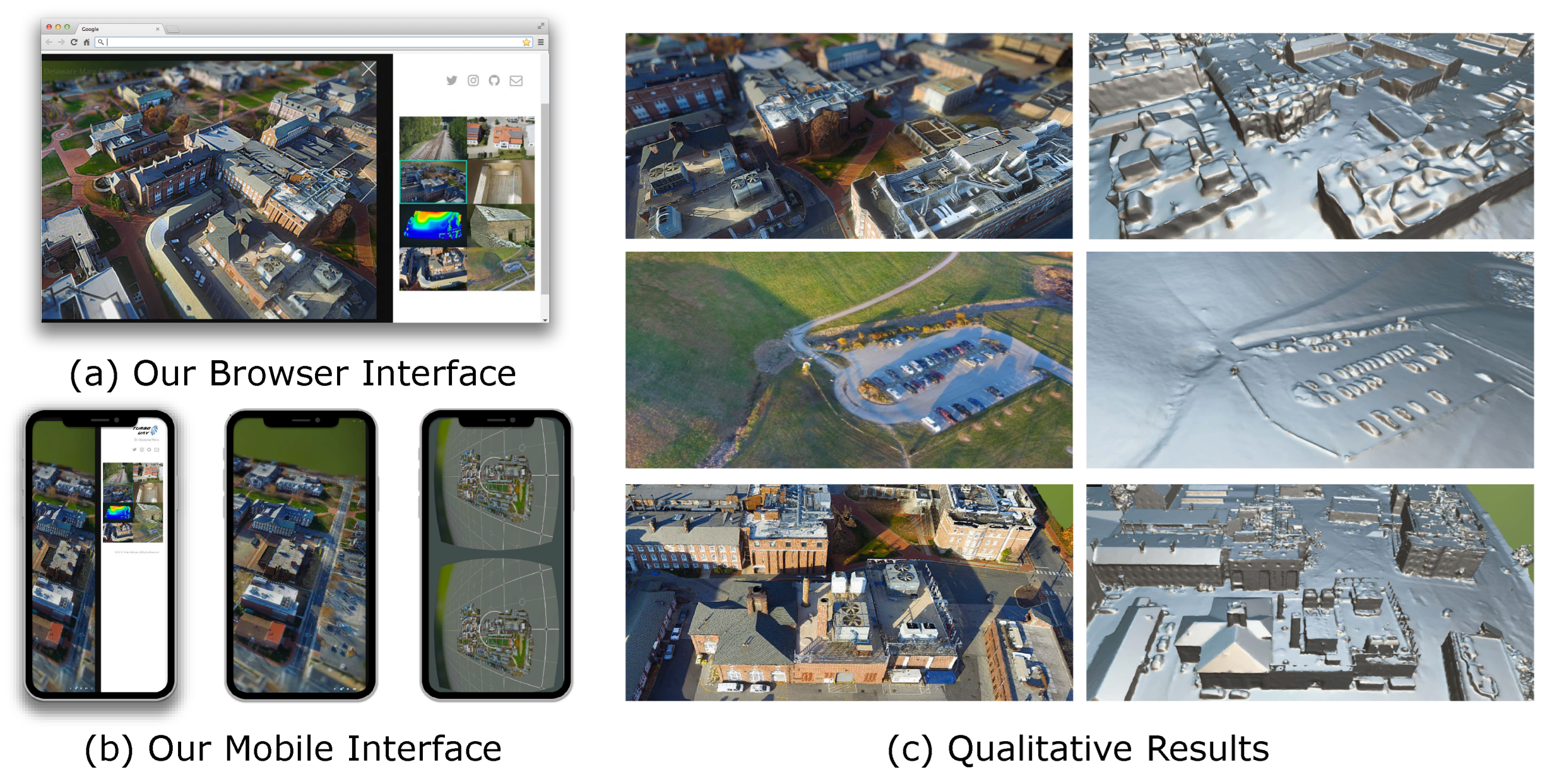
We tested the CUDA accelerated BP algorithm with the maximum iteration set to 5 and the maximum disparity value set to 16. We set both the spatial and range filter size of the JBF to 15 and the diameter of the filtering neighborhood to 10 pixels. We divide the imaging plane to a grid and calculate Harris corners inside each grid individually to prevent too many points detected at the same region given a hard threshold. We fly at 100 meters with a speed of 3 m/s and maintain altitude using the DJI built-in NAZA flight controller. We choose two frames out of every 10 frames to form a virtual stereo camera. The baseline is approximately 0.5 meters. We conducted experiments in various environments and upload the results to Sketchfab [36]. We set the field of view (FOV) to 60 degrees, physically based rendering (PBR) to “shadeless”, and enable additional depth of field (DoF), bloom, and Reinhard tone mapping effects. We also construct a dynamic web portal for navigation, preview, and management of the uploaded 3D models.
4.2. High Resolution Reconstruction Experiments
In order to assess the upper bound of our reconstruction quality, we have also carried out experiments using a more recent consumer drone, namely the DJI Mavic 3 equipped with the Hasselblad L2D-20c 4/3 CMOS 20-megapixel aerial camera. This particular camera features a 24mm equivalent focal length lens and an adjustable aperture ranging from f/2.8 to f/11, providing a native dynamic range of 12.8 stops. For flight path planning and image capture, we utilized the publicly available Map Pilot Pro application. Our experimentation took place at the Montalvo Arts Center in Saratoga, California.
The results obtained from our proposed algorithm exhibit superiority in both texture and geometric accuracy when compared to the Google Maps 3D reconstruction. Despite the inherent advantage of Google Maps employing satellite imagery for large-scale 3D reconstruction, our utilization of UAV drones presents a noteworthy advantage due to the close proximity of data capture. The reduced distance from the target scene allows for enhanced resolution and finer detail acquisition. Moreover, this advantage is complemented by the cost-effectiveness of our approach. The deployment of UAV drones is considerably more economical than satellite-based methods, making our algorithm not only superior in terms of texture and geometric accuracy but also economically viable for widespread implementation. This cost-effectiveness renders our 3D reconstruction algorithm an attractive option for various applications, particularly those with limited financial resources, and further underscores its significance in the domain of geographical mapping and remote sensing technologies.
Figure 3.
Qualitative results on the reconstructed 3D scenes. Note that the VR view shown in (b) and the mesh rendered in (c) are provided by Sketchfab [36].
Figure 3.
Qualitative results on the reconstructed 3D scenes. Note that the VR view shown in (b) and the mesh rendered in (c) are provided by Sketchfab [36].
4.3. Auto Labeling and Measurements
We seek to automatically label the 3D point cloud, using open source OpenStreetMap (OSM) [37] geographical mapping tool. For the OSM users, given a GPS boundary request, the OSM API server returns an XML file containing tags represented by various data structures (nodes, ways, and relations). Each tag describes a geographic attribute, including roads, buildings, water, vegetation, etc. The boundaries are represented by a polygon based on GPS coordinates. We consider generating an orthographic projection from the 3D point cloud and align with the OSM map file to achieve automatic labeling of the 3D scene object segments. We first perform a RANSAC-based plane detection method to extract the ground plane and define the normal direction of the plane to be the Z axis. We translate the 3D point cloud to Z=0 and place a virtual orthographic camera is placed at center +Z direction such that all points are covered in the camera view. Next, we render the scene to obtain an orthophoto as well as a depth map stored in the Z-buffer. Once the orthophoto is obtained, we send GPS coordinates recorded by the original image to request a RGB satellite image from the Google Maps API. SIFT descriptors are extracted from both images and matched against each other. Again, we apply RANSAC to solve for scale, rotation and translation to align the orthophoto with the satellite image. This fully automated process givens us (pixel accurate) high precision coordinates of our reconstructed mesh. Next, we filter all objects less than 5 meters in height to obtain building segmentation masks as shown in Figure 4. To validate the accuracy of our approach, we manually label 12 main buildings from the University of Delaware using Google Earth Pro, obtaining the groundtruth areas and perimeters of each building. The measurements obtained from our automatic pipeline closely match the groundtruth data, as presented in Table 1, establishing the precision of our 3D reconstruction pipeline. The final reconstruction results are presented in Figure 5.
In conclusion, our method demonstrates remarkable accuracy in automatically labeling 3D point clouds, incorporating orthophotos aligned with satellite imagery. The close agreement between our automated measurements and groundtruth data underscores the effectiveness of our pipeline, offering great potential for various applications in geographic mapping and 3D scene analysis.
4.4. Flight Path planning
Automatic flight path planning plays a pivotal role in ensuring efficient and safe operation of UAVs in various applications. We import the point clouds data obtained from Section 3.3 into the Robot Operating System (ROS) [38] and leverage state-of-the-art algorithm [39] for trajectory planning. Given any target 3D point in space, the algorithm can generate a trajectory that allows the UAV to autonomously navigate through complex environments with enhanced precision (See Figure 4b). This paper underscores the necessity of automated flight path planning by elucidating how our proposed methodology harnesses the power of real-time point cloud data and advanced trajectory planning techniques to enable UAVs to effectively navigate through intricate spaces, thereby bolstering the reliability and versatility of UAV operations across a spectrum of real-world scenarios. Furthermore, the integration of automatic flight path planning with point cloud data can facilitate task-level UAV command and streamline fleet operations, paving the way for coordinated and collaborative missions with multiple UAVs operating seamlessly in real-world environments. Notably, this approach enables a unique strategy where one drone can be designated to fly at a higher altitude for 3D mapping purposes, subsequently providing other drones with essential 3D map information. These secondary drones can then leverage this map data for low-altitude optimal trajectory planning and obstacle avoidance, enhancing overall operational efficiency and safety during complex missions.
5. Discussion
We show quantitative results in Table 1 and compare with ground-truth measurement data. As can be seen from Table 1, our method achieves highly precise results across different building structures. Qualitative results from Figure 5 and Figure 6 show superiority in both texture and geometric quality when compared to the Google Maps 3D reconstruction. We also demonstrate useful applications such as fully automated labeling of buildings, building measurements, and flight path planning.
A crucial challenge in the current photogrammetry pipelines is the significant processing time required to fully analyze the captured imagery data, thereby constraining the real-time data acquisition capability. Such rapid data acquisition is indispensable in scenarios like onsite scanning, emergency response, and planning. An optimal scanning pipeline should ideally enable real-time scene mapping as the drone follows its flight path, allowing inspectors to assess partial scans even before the flight mission concludes. However, the high time complexity of traditional photogrammetry approaches makes it inapplicable to achieve these objectives.
Our proposed approach emphasizes the utilization of high-efficiency algorithms with minimal computational burden at each pipeline stage. Notably, we employ the Harris corner detector for feature extraction, as opposed to more resource-intensive options like SIFT or SURF descriptors. For stereo matching, we adopt real-time Belief Propagation (BP) on downsampled images, diverging from the resource-demanding full-resolution multi-view stereo matching. Furthermore, we opt for the expedited EPnP algorithm for camera pose estimation/refinement instead of the conventional Bundle Adjustment (BA) technique found in many SfM pipelines. Finally, we derive a constant speed model using the Kalman filter to improve the pose estimation accuracy. The culmination of these choices results in our system’s remarkable capability to generate accurate dense point clouds in near real-time, achieving a consistent speed of 25 frames per second.
6. Conclusions
We have presented an efficient, near-real-time solution for 3D reconstruction using off-the-shelf consumer UAVs. Our proposed alternative approach addresses the limitations of current photogrammetry pipelines for real-time mapping using consumer-level camera drones. By employing high-efficiency algorithms with minimal computational cost at each step of the pipeline, we have achieved significant advancements in real-time 3D reconstructions. Our method conducts feature extraction, verification, camera poses estimation/refinement, and dense stereo simultaneously on a frame-by-frame basis, allowing for incremental and online mapping. This is in contrast to conventional approaches that rely on global optimization and require the entire dataset as input, hindering real-time capabilities.
Our approach holds great promise for various applications, including onsite scans and inspections, emergency response, and planning. The ability to examine partial scans even before completing the flight mission is a significant advantage, enhancing decision-making and operational efficiency. Moreover, the real-time data acquisition achieved by our method opens up new possibilities for micro UAVs in diverse industries, such as agriculture, construction, transportation, and film-making, where rapid and cost-effective mapping solutions are increasingly in demand.
While our method has demonstrated remarkable performance, further research and development are necessary to continue refining and expanding its capabilities. Future work could focus on optimizing algorithms even further, exploring different feature extraction and matching techniques, and investigating ways to handle challenging imaging conditions more effectively. Also, we plan to compare the proposed approach with other methods on 3D reconstruction benchmark datasets and add more global/loop-closure constraints to minimize trajectory errors. Additionally, we would like to validate the method’s accuracy and robustness in various real-world scenarios to speed up its engineering adoption and deployment.
In conclusion, our work represents a significant step towards unlocking the full potential of consumer-level camera drones for real-time high-resolution mapping, offering promising prospects for enhanced efficiency and productivity across numerous industries.
References
- Harris, C.G.; Stephens, M.; et al. A combined corner and edge detector. In Proceedings of the Alvey vision conference; Citeseer. 1988; Volume 15, pp. 10–5244. [Google Scholar]
- Lowe, D.G. Object recognition from local scale-invariant features. In Proceedings of the Proceedings of the seventh IEEE international conference on computer vision. 1999; Volume 2, pp. 1150–1157. [Google Scholar]
- Bay, H.; Tuytelaars, T.; Van Gool, L. Surf: Speeded up robust features. In Proceedings of the Computer Vision–ECCV 2006: 9th European Conference on Computer Vision, Graz, Austria, 7-13 May 2006; Proceedings, Part I 9. Springer, 2006; pp. 404–417. [Google Scholar]
- Lepetit, V.; Moreno-Noguer, F.; Fua, P. Epnp: An accurate o (n) solution to the pnp problem. International journal of computer vision 2009, 81, 155. [Google Scholar] [CrossRef]
- Triggs, B.; McLauchlan, P.F.; Hartley, R.I.; Fitzgibbon, A.W. Bundle adjustment—a modern synthesis. In Proceedings of the Vision Algorithms: Theory and Practice: International Workshop on Vision Algorithms Corfu, Greece, 21–22 September; 1999 Proceedings. Springer, 2000; pp. 298–372. [Google Scholar]
- Agarwal, S.; Furukawa, Y.; Snavely, N.; Simon, I.; Curless, B.; Seitz, S.M.; Szeliski, R. Building rome in a day. Communications of the ACM 2011, 54, 105–112. [Google Scholar] [CrossRef]
- Civera, J.; Grasa, O.G.; Davison, A.J.; Montiel, J.M. 1-Point RANSAC for extended Kalman filtering: Application to real-time structure from motion and visual odometry. Journal of field robotics 2010, 27, 609–631. [Google Scholar] [CrossRef]
- Yoon, K.J.; Kweon, I.S. Locally adaptive support-weight approach for visual correspondence search. In Proceedings of the 2005 IEEE Computer Society Conference on Computer Vision and Pattern Recognition (CVPR’05); 2005; Volume 2, pp. 924–931. [Google Scholar]
- Hirschmuller, H. Stereo processing by semiglobal matching and mutual information. IEEE Transactions on pattern analysis and machine intelligence 2007, 30, 328–341. [Google Scholar] [CrossRef] [PubMed]
- Geiger, A.; Roser, M.; Urtasun, R. Efficient large-scale stereo matching. In Computer Vision–ACCV 2010; Springer, 2011; pp. 25–38. [Google Scholar]
- Hosni, A.; Rhemann, C.; Bleyer, M.; Rother, C.; Gelautz, M. Fast cost-volume filtering for visual correspondence and beyond. IEEE transactions on pattern analysis and machine intelligence 2012, 35, 504–511. [Google Scholar] [CrossRef] [PubMed]
- Boykov, Y.; Veksler, O.; Zabih, R. Fast approximate energy minimization via graph cuts. IEEE Transactions on pattern analysis and machine intelligence 2001, 23, 1222–1239. [Google Scholar] [CrossRef]
- Sun, J.; Zheng, N.N.; Shum, H.Y. Stereo matching using belief propagation. IEEE Transactions on Pattern Analysis and Machine Intelligence 2003, 25, 787–800. [Google Scholar]
- Yang, Q.; Wang, L.; Yang, R.; Stewénius, H.; Nistér, D. Stereo matching with color-weighted correlation, hierarchical belief propagation, and occlusion handling. IEEE transactions on pattern analysis and machine intelligence 2008, 31, 492–504. [Google Scholar] [CrossRef] [PubMed]
- Kolmogorov, V.; Zabin, R. What energy functions can be minimized via graph cuts? IEEE transactions on pattern analysis and machine intelligence 2004, 26, 147–159. [Google Scholar] [CrossRef] [PubMed]
- Felzenszwalb, P.F.; Huttenlocher, D.P. Efficient belief propagation for early vision. International journal of computer vision 2006, 70, 41–54. [Google Scholar] [CrossRef]
- Yang, Q.; Wang, L.; Ahuja, N. A constant-space belief propagation algorithm for stereo matching. In Proceedings of the 2010 IEEE Computer Society Conference on Computer Vision and Pattern Recognition; 2010; pp. 1458–1465. [Google Scholar]
- Klein, G.; Murray, D. Parallel tracking and mapping for small AR workspaces. In Proceedings of the 2007 6th IEEE and ACM international symposium on mixed and augmented reality; 2007; pp. 225–234. [Google Scholar]
- Mur-Artal, R.; Montiel, J.M.M.; Tardos, J.D. ORB-SLAM: a versatile and accurate monocular SLAM system. IEEE transactions on robotics 2015, 31, 1147–1163. [Google Scholar] [CrossRef]
- Newcombe, R.A.; Lovegrove, S.J.; Davison, A.J. DTAM: Dense tracking and mapping in real-time. In Proceedings of the 2011 international conference on computer vision; 2011; pp. 2320–2327. [Google Scholar]
- Engel, J.; Koltun, V.; Cremers, D. Direct sparse odometry. IEEE transactions on pattern analysis and machine intelligence 2017, 40, 611–625. [Google Scholar] [CrossRef]
- Engel, J.; Schöps, T.; Cremers, D. LSD-SLAM: Large-scale direct monocular SLAM. In Proceedings of the European conference on computer vision. Springer; 2014; pp. 834–849. [Google Scholar]
- Gherardi, R.; Farenzena, M.; Fusiello, A. Improving the efficiency of hierarchical structure-and-motion. In Proceedings of the 2010 IEEE computer society conference on computer vision and pattern recognition; 2010; pp. 1594–1600. [Google Scholar]
- Schonberger, J.L.; Frahm, J.M. Structure-from-motion revisited. In Proceedings of the IEEE conference on computer vision and pattern recognition; 2016; pp. 4104–4113. [Google Scholar]
- Wilson, K.; Snavely, N. Robust global translations with 1dsfm. In Proceedings of the Computer Vision–ECCV 2014: 13th European Conference, Zurich, Switzerland, 6-12 September 2014; Proceedings, Part III 13. Springer, 2014; pp. 61–75. [Google Scholar]
- Rosten, E.; Porter, R.; Drummond, T. Faster and better: A machine learning approach to corner detection. IEEE transactions on pattern analysis and machine intelligence 2008, 32, 105–119. [Google Scholar] [CrossRef]
- Bhardwaj, A.; Sam, L.; Bhardwaj, A.; Martín-Torres, F.J. LiDAR remote sensing of the cryosphere: Present applications and future prospects. Remote Sensing of Environment 2016, 177, 125–143. [Google Scholar] [CrossRef]
- Bolourian, N.; Hammad, A. LiDAR-equipped UAV path planning considering potential locations of defects for bridge inspection. Automation in Construction 2020, 117, 103250. [Google Scholar] [CrossRef]
- Zhang, Z. A flexible new technique for camera calibration. IEEE Transactions on pattern analysis and machine intelligence 2000, 22, 1330–1334. [Google Scholar] [CrossRef]
- Bradski, G. The openCV library. Dr. Dobb’s Journal: Software Tools for the Professional Programmer 2000, 25, 120–123. [Google Scholar]
- Wang, Q.; Yu, Z.; Rasmussen, C.; Yu, J. Stereo vision–based depth of field rendering on a mobile device. Journal of Electronic Imaging 2014, 23, 023009. [Google Scholar] [CrossRef]
- Kopf, J.; Cohen, M.F.; Lischinski, D.; Uyttendaele, M. Joint bilateral upsampling. In Proceedings of the ACM Transactions on Graphics (ToG); 2007; Volume 26, p. 96. [Google Scholar]
- ICPCUDA Open Source Utility Library. https://github.com/mp3guy/ICPCUDA.
- Kazhdan, M.; Hoppe, H. Screened poisson surface reconstruction. ACM Transactions on Graphics (ToG) 2013, 32, 1–13. [Google Scholar] [CrossRef]
- Waechter, M.; Moehrle, N.; Goesele, M. Let there be color! Large-scale texturing of 3D reconstructions. In Proceedings of the European conference on computer vision; Springer, 2014; pp. 836–850. [Google Scholar]
- Sketchfab. https://sketchfab.com.
- Haklay, M.; Weber, P. Openstreetmap: User-generated street maps. IEEE Pervasive computing 2008, 7, 12–18. [Google Scholar] [CrossRef]
- Quigley, M.; Conley, K.; Gerkey, B.; Faust, J.; Foote, T.; Leibs, J.; Wheeler, R.; Ng, A.Y.; et al. ROS: an open-source Robot Operating System. In Proceedings of the ICRA workshop on open source software; 2009; p. 5. [Google Scholar]
- Zhou, B.; Gao, F.; Pan, J.; Shen, S. Robust real-time uav replanning using guided gradient-based optimization and topological paths. In Proceedings of the 2020 IEEE International Conference on Robotics and Automation (ICRA); 2020; pp. 1208–1214. [Google Scholar]
Figure 4.
Demonstration of UAV applications. (a) Automatic building segmentation results. The ground plane is marked in green and the segmented 3D buildings are coded in random color (see Section 4.3). (b) Automatic flight path planning on the point cloud. The purple 3D path shows the planned flight trajectory between the current location and the target. (see Section 4.4)

Figure 5.
Qualitative results between our 3D model and Google Earth. Note that the viewpoints are manually adjusted to roughly align with each other. Our method is highly efficient while performing favorably against Google Earth in terms of final reconstruction quality.
Figure 5.
Qualitative results between our 3D model and Google Earth. Note that the viewpoints are manually adjusted to roughly align with each other. Our method is highly efficient while performing favorably against Google Earth in terms of final reconstruction quality.
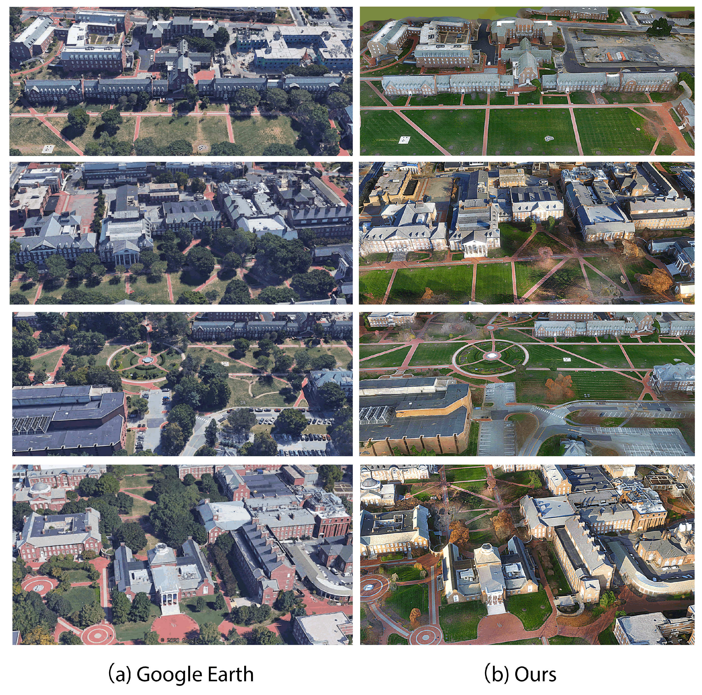
Figure 6.
High-Resolution Reconstruction Experiments. We reconstructed the Montalvo Arts Center (Saratoga, California) using a more recent consumer drone equipped with a 20-megapixel aerial camera 4.2. Row 1 to 4 shows the reconstructed mesh and 3D model with zoom-in views. Note that the zoom level is more than 10X. Row 5 shows the same 3D building visualization in Google Maps. Our results exhibit much-improved quality in both texture and geometry details.
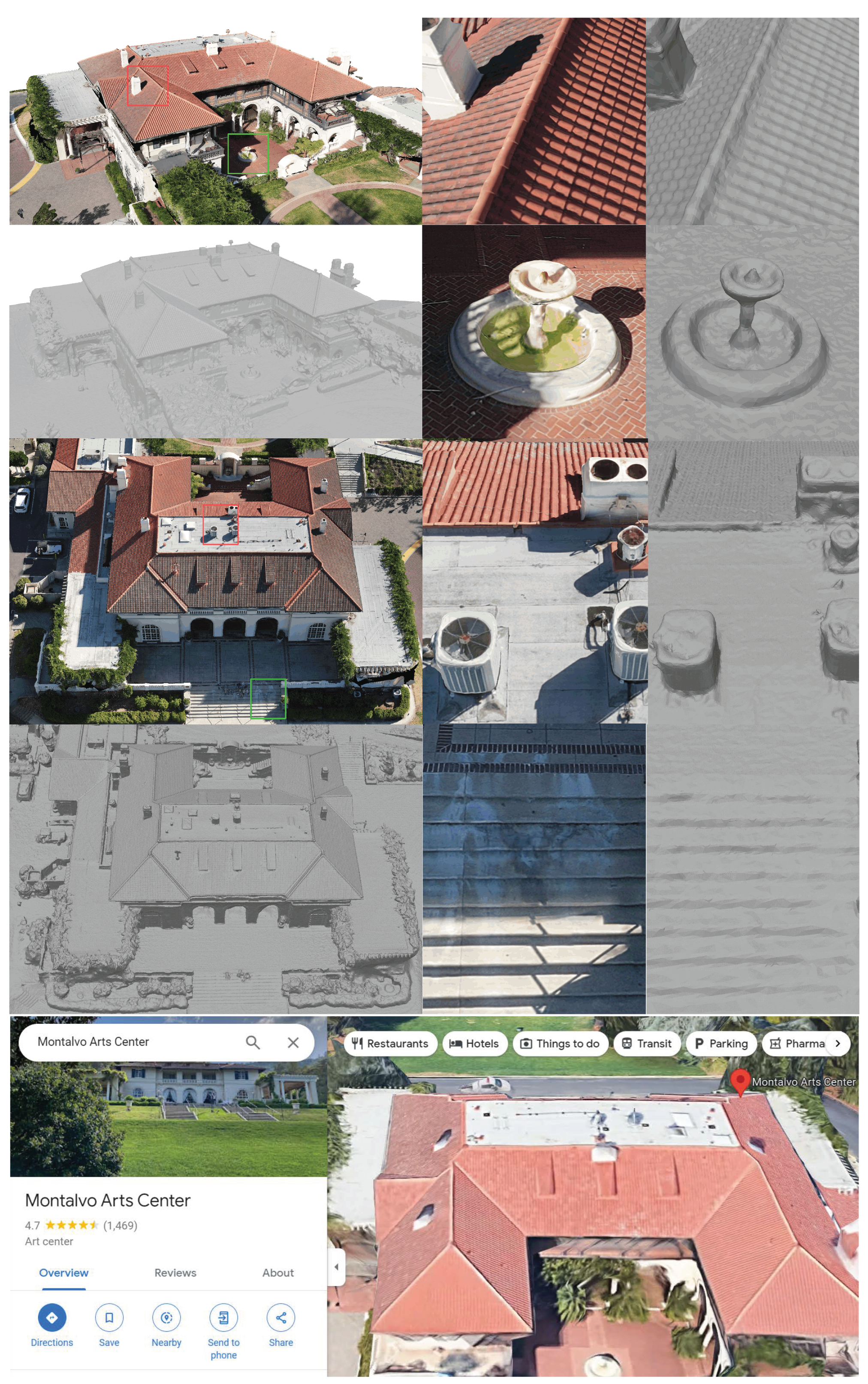

Table 1.
Automatic measurement results on buildings from the University of Delaware. GTArea and GTPerim denote the ground truth area and perimeter. The camera settings column shows the shutter speed (in seconds) and ISO value. The detailed measurement process is outlined in Section 4.3.
Table 1.
Automatic measurement results on buildings from the University of Delaware. GTArea and GTPerim denote the ground truth area and perimeter. The camera settings column shows the shutter speed (in seconds) and ISO value. The detailed measurement process is outlined in Section 4.3.
| Morris Library | 7047.85 | 7000.00 | 389.69 | 390.00 | 1.12 | 1/300, 100 |
| Memorial Hall | 2458.78 | 2440.00 | 281.84 | 280.00 | 0.63 | 1/300, 100 |
| Hullihen Hall | 2368.23 | 2320.00 | 195.80 | 196.00 | 0.63 | 1/300, 100 |
| Mitchell Hall | 1091.59 | 1080.00 | 169.54 | 168.00 | 0.55 | 1/300, 100 |
| Gore Hall | 2781.18 | 2760.00 | 224.43 | 224.00 | 0.65 | 1/300, 100 |
| Sharp Laboratory | 2652.83 | 2620.00 | 294.71 | 292.00 | 0.62 | 1/300, 100 |
| Wolf Hall | 2599.18 | 2560.00 | 300.32 | 296.00 | 0.68 | 1/150, 200 |
| Du Pont Hall | 3886.30 | 3840.00 | 341.62 | 338.00 | 0.73 | 1/150, 200 |
| Evans Hall | 2638.77 | 2600.00 | 206.14 | 204.00 | 0.69 | 1/150, 200 |
| Brown Lab | 4690.47 | 4640.00 | 298.94 | 296.00 | 0.82 | 1/150, 200 |
| Lammot du Pont Lab | 1533.21 | 1520.00 | 186.15 | 184.00 | 0.64 | 1/60, 400 |
| Robinson Hall | 768.33 | 764.00 | 119.84 | 118.00 | 0.45 | 1/60, 400 |
Disclaimer/Publisher’s Note: The statements, opinions and data contained in all publications are solely those of the individual author(s) and contributor(s) and not of MDPI and/or the editor(s). MDPI and/or the editor(s) disclaim responsibility for any injury to people or property resulting from any ideas, methods, instructions or products referred to in the content. |
© 2023 by the authors. Licensee MDPI, Basel, Switzerland. This article is an open access article distributed under the terms and conditions of the Creative Commons Attribution (CC BY) license (http://creativecommons.org/licenses/by/4.0/).
Copyright: This open access article is published under a Creative Commons CC BY 4.0 license, which permit the free download, distribution, and reuse, provided that the author and preprint are cited in any reuse.


