Estimating model for COVID-19 Infected Cases and Deaths in Tamil Nadu State

1. Introduction

1.1. Study Background

The coronavirus epidemic that beginning in Wuhan city (China) on December 31, 2019 and has since evolved into a pandemic. The incidence of novel COVID-19 infections has dramatically grown in the absence of antiviral medications and vaccinations, resulting in huge economic losses, panic and many deaths.

The use of different statistical models to analyse epidemic data has emerged as a key study field for predicting number of COVID-19 deaths and coronavirus-infected individuals.

The numerical data relevant to certain samples or groups are represented by statistical models. In order to assess trends in the data shown, these models frequently take the form of line graphs and scatterplots. While statistical models may display data in a variety of scenarios, those that deal with COVID-19 are particularly well-liked in the present since they provide numerical information about this pandemic, such as the number of cases as well as deaths brought on by COVID-19. These models have also proved very helpful in locating cases throughout the globe to specific nations, regions, cities, and specific areas within cities, enabling the authorities in these locations to respond appropriately to the infection. Additionally, models have focused on a variety of crucial traits among individuals who present with COVID-19, such as age, race, gender, and pre-existing diseases. This enables researchers to determine which populations are most at danger from this pandemic [1].

AI (Artificial Intelligence) techniques built on ML (Machine Learning) and mathematical models are being utilised to evaluate the type of the epidemic’s progress throughout each country and identify any potential amplifying factors that might impede its effects [2].

1.2. Literature Review

In order to examine the relationship between dependent and independent variables and determine the current rate of corona virus spread, [3] sought to build on earlier research. This research statistically analysed the relationship of factors like region, sex, birth year, infection date, and release date or decease with the noted number of recovered as well as died patients. The findings revealed that region, infection date, and sex were associated with the number of both recovered and died patients, whereas birth year was associated with the number of died patients only. Furthermore, no deaths from COVID were noted among released patients, whereas 11.3 percent of died patients were confirmed to be COVID positive after their deaths. In South Korea, the main factor associated with infection numbers was found to be the number of patients infected by an unknown source, representing more than 33% of total infected patients.

The association between the overall number of COVID-19 infections and recoveries in various countries was studied and analysed by [4] using the chain-binomial variant of Bailey’s model. They also pointed out that most studies have investigated COVID-19 cases with different regression as well as time series models, which are commonly used to assess the trend or growth of any illness.

The relationship between the transmission of viral infections and human migration was investigated by [5]. They concluded that the intensity of pedestrian traffic in the research period impacted the virus spread after 15-20 days on average.

A time series-based system to track epidemics is a term that [6] aimed to create. Utilizing univariate time series models, he showed the evolution of the reported incidents in the first stage. Additionally, he combined the models to offer more precise and reliable findings and thought about statistical probability distributions to create hypothetical futures. The “time series susceptible-infected-recovered” [tsiR] model was created and used as last stage, and its epidemiological ratio (R₀) was calculated to determine when the epidemic ended. Time series models used comprised the traditional exponential smoothing along with ARIMA techniques, in addition to feed-forward ANN (“Artificial Neural Networks”) and MARS (“Multivariate Adaptive Regression Splines”) from the ML toolbox. The basic mean, Granger-Newbold, and Bates-Granger techniques were included in the combinations. To assess the spread and containment of the epidemic, the tsiR model as well as the R₀ ratio was applied. The recommended method was applied to monitor the COVID-19 outbreak in Greece.

Using Bailey’s model and secondary data, [7] calculated the removal rate, or the percentage of eliminated individuals in the infected population. Additionally, regression analysis was done to demonstrate the linear association between this indicator and the frequencies of all infections. Finally, they discussed the connection between the model and decision-making.

By carefully analyzing the cases that had been reported in the country up until 22 April 2020, [8] used exploratory data analysis to create a statistical model that would help people understand the Corona virus in India. The study’s findings illustrated the daily and weekly effects of COVID-19 in India and drew comparisons between that nation and its neighbours as well as other badly afflicted nations.

The impact of travel history and interaction with travellers on the dissemination of the corona virus in Nigeria was evaluated by [9] using the OLS ("Ordinary Least Squares") estimator. They created predictions with extracting data from the NCDC (“Nigeria Centre for Disease Control”) website spanning March 31, 2020, to May 29, 2020. The model evaluated the time before and after the Nigeria federal government imposed travel restrictions. Based on the diagnostic checks performed, the fitted model had good fit to dataset and no validity violations. With travel history as well as contact with travellers observed to rise likelihood of coronavirus infection by 85 and 88%, the results demonstrate that govt. made the right selection in enforcing travel restrictions. The authors came to the conclusion that the govt must enforce this policy to contain Coronavirus.

Using stochastic modeling, [10] forecasted the prevalence of COVID-19 trends in East African countries, with a focus on Somalia, Sudan, Djibouti, and Ethiopia. The study’s findings indicated that, under the average rate scenario, the number of coronavirus positive individuals in Ethiopia might increase range between 5,846 to 56,610 within four months after 30 June, 2020.

An "autoregressive distributed lag model and limits Cointegration tests" were used by [11] to evaluate the long-run equilibrium relationship between the cumulative number of new COVID-19 infections (X) and the cumulative number of fatalities brought on by COVID-19 (Y).The stability of the calculated model was also assessed. The consistency of the model parameters is evaluated using both the cumulative sum of recursive residuals test and squares test.

The dynamic relationship between NCASE and DEATH was examined by [12] using the VECM ("Vector Error Correction Model"), Johnsen-Fisher Cointegration test, and the "Granger causality" test. From 1 April 2020 to 26 December 2010, data on daily new COVID-19-infected cases along with COVID-19 related deaths in the India, Ukraine, Canada, and United States have been gathered from the website. Summary figures showed that the United States had the largest number of instances of COVID-19 infection, followed by India, Canada, and Ukraine. The US also had the highest number of COVID-19-related deaths, followed by India, Ukraine, and Canada. Canada leads all other countries in terms of the death rate, followed by the US, Ukraine, as well as India. Results of the Johnsen-Fisher Cointegration test indicate that there is only one Cointegration equation. The Granger causality test and the VECM demonstrate that there is a short & long-term causal correlation between COVID-19 infection and mortality instances. It is discovered that the rate of adjustment is 9.9%.

1.3. Objectives of the Present Study

This study aims to determine the relations and trends between the number of COVID-19 deaths (DEATH) and number of new COVID-19 infections (NCASE) in all 37 regions of Tamil Nadu (India) in the month of August 2020 based on the foregoing discussion. A panel regression model will be used, with DEATH serving as the dependent variable and NCASE serving as the “independent variable”.

1.4. Panel Data Model

These are a sort of data that include observations of various events gathered over various time scales for same group of people, entities, or units. Econometric panel data, in a nutshell, are multidimensional data gathered over a certain time.

A simple “regression model” of panel data is defined as

$$Y_{it}=\alpha +\beta X_{it}+v_{it}$$

where ${\nu }_{it}={\gamma }_i{\nu }_{i(t-1)}+{\mu }_{it}$present predicted residuals obtained from panel regression analysis where, Y represents dependent variable, X denotes explanatory or independent variable, $\alpha$and$\beta$indicates intercept and slope, t for the t^th time period, and i represents i^th cross-sectional unit and X is considered to be non-stochastic as well as error term to follow the “classical assumptions”, i.e., $E(v_{it})=N(0,{\sigma }^2)$. In the present research, the number of cross-sections (districts) is 37 (i=1, 2, 3,..., 37), and the number of time points is 1, 2, 3,..., 30.

Panel data modelling detailed discussions may be observed in, viz., [13,14,15,16,17].

Panel data give “more informative data, more variability, less collinearity among variables, more degrees of freedom and more efficiency” because they combine time series of cross-sectional observations, [14].

2. Materials and Methods

2.1. Materials

The COVID-19 infected and deaths dataset of month of August, 2020, related to all 37 regions of Tamil Nadu, India was gathered from the Tamil Nadu govt official website. The research objectives of the current study were examined using a variety of econometric methodologies linked to panel data regression modelling. The techniques section discusses several panel data regression modelling strategies. Model and parameter estimates was done using EViews Ver. 11.

Models based on panel data provide descriptions of individual behaviour across time and across individuals. Pooled models (OLS regression) or Constant Coefficient Models (CCM), RE (Random Effects) and FE (Fixed Effects) models are the three different types of models.

2.2.1. Unit Root Tests

LM (Lagrange Multiplier) stationarity [15] or the [16] test the may be used to check for unit roots inside panel data. The alternative hypothesis is that the panels are stationary, wheras null hypothesis is that they have unit roots. Based on the findings, one could accept the alternative hypothesis as well as reject null hypothesis if the p value is <0.05.

2.2.2. OLS Regression (Pooled Model) or CCM

Cross-sectional analysis often makes the following assumptions about the pooled model with constant coefficients:

$$Y_{it}=\alpha +\beta X_{it}+v_{it}$$

where, i=1,2,3, …, 37, & t= 1,2,3, …,31, here i stands for i^th cross-sectional units as well as t for the t^th time period, and it is considered that X indicates a non-stochastic and error term follows “classical assumptions”, i.e.,.

$$E(v_{it})~N(0,{\sigma }^2)$$

2.2.3. Individual-Specific Effects Model

We suppose that the people that were captured ${\alpha }_i$exhibit unobserved heterogeneity. The fundamental question is if there is a relationship between the individual-specific effects${\alpha }_i$and the regressor. A FE model exists if they are linked. A RE model exists if they are not correlated.

2.2.4. FE LSDV (Least Squares Dummy Variable) Model [17]

The phrase "fixed effects" is applied since every entity’s intercept does n’t fluctuate with time; it is therefore time invariant, although the intercept might change among districts.

$$y_{it}=\alpha +x_{it}\beta +{\gamma }_{it}$$

After estimating, one may obtain the person-specific result as

$$\widehat{{\alpha }_i}={\overline{y}}_i-{\overline{x}}_i\widehat{\beta }$$

In other terms, individual-specific impacts are the residual variance in the “dependent variable” that the regressor is unable to account for. The fixed effects intercept might differ amongst the districts when utilising the dummy variable approach.

2.2.5. RE Model

It is assumed that the regressor is not affected by the individual-specific effects${\alpha }_i$, which are included ${\alpha }_i$in error term. The composite error term and slope parameters are the same for each person i.e.,${\epsilon }_{it}={\alpha }_i+v_{it}$.

$$y_{it}=x_{it}\beta +({\alpha }_i+v_{it})$$

Here $\mathrm{var}({\epsilon }_{it})={\sigma }_{\alpha }{}^2+{\sigma }_v{}^2$and$\mathrm{cov}({\epsilon }_{it},{\epsilon }_{is})={\sigma }_{\alpha }{}^2$so ${\rho }_{\epsilon }=cor({\epsilon }_{it},{\epsilon }_{is})=\frac{{\sigma }_{\alpha }{}^2}{{\sigma }_{\alpha }{}^2+{\sigma }_{\epsilon }{}^2}$

Rho indicates the error’s interclass correlation, or the percentage of its variation accounted for by person-specific effects. If the individual effects exceed the idiosyncratic mistake, it becomes closer to 1.

2.2.6. Hausman Test

The RE model is favoured, which is the null hypothesis of given test and the FE model is favoured, which is the alternative hypothesis. The “null hypothesis” is that there is no correlation between the regressor and the$({\alpha }_i)$, and this test checks for that relationship. If the Hausman test [18] suggests using the RE estimator, one should do so since it is more effective. Only the time-varying regressors could be used to calculate the Hausman test statistic.

$$H={({\widehat{\beta }}_{RE}-{\widehat{\beta }}_{FE})}^{|}(V({\widehat{\beta }}_{RE})-V({\widehat{\beta }}_{FE})({\widehat{\beta }}_{RE}-{\widehat{\beta }}_{FE})$$

2.2.7. Wald Test

The Wald test [19] is used to determine which model variables significantly contribute to the observed impact. The test, also known as the “Wald chi-squared test”, could be utilised to examine if explanatory variables within a model are important, namely, whether they add to the model’s explanatory power. Variables with no explanatory power could be removed from the model without having any significant influence. Some parameter equals some value is the test’s null hypothesis.

3. Results and Discussions

3.1. Unit Root Tests

It is crucial for time series data studies that the research variables remain stationary, which indicates that the variable data’s variances and means are same. “Levin-Lin-Chu unit root tests” were performed in order to determine if the research variables—namely, NCASE and the DEATH were stationary. Table 1 present the findings.

Table 1. Unit root test outcomes for variable DEATH and NCASE.

Varibles	NCASE	DEATH
Method	Levin, Lin & Chu t*
Statistic	-8.62523	-8.66106
Prob**	0.0000	0.0000

** Probabilities are calculated supposing asymptotic Normality.

Table 1. Unit root test outcomes for variable DEATH and NCASE.

Varibles	NCASE	DEATH
Method	Levin, Lin & Chu t*
Statistic	-8.62523	-8.66106
Prob**	0.0000	0.0000

** Probabilities are calculated supposing asymptotic Normality.

The NCASE and DEATH variables are shown to be stationary in level in Table 1 test findings because the method are shown to be highly significant (p<0.0000). As a result, it is determined that the analysis’s variables are stationary.

3.2. Summary Statistics

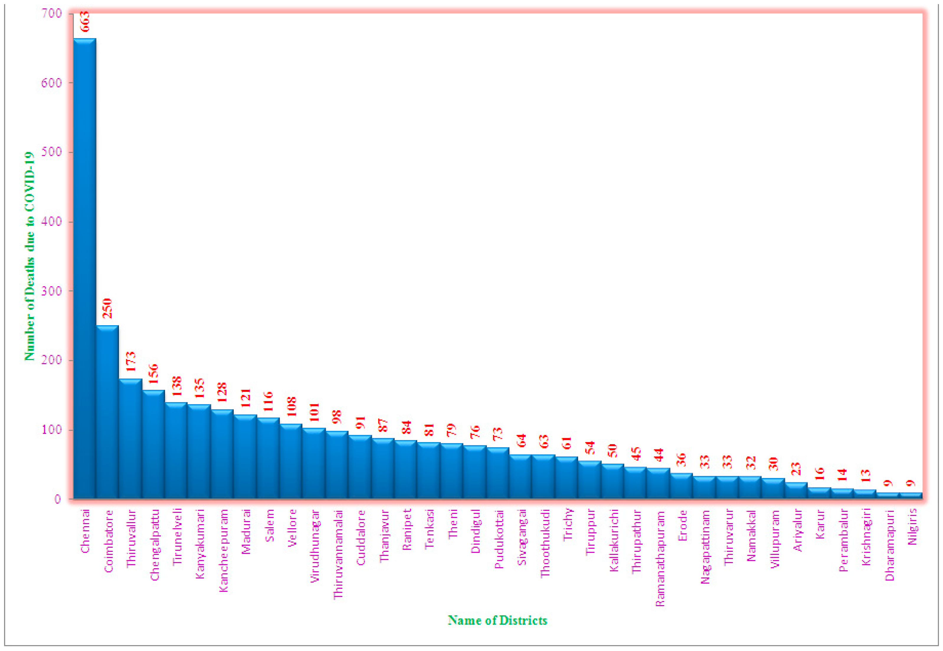
Positive patients of COVID-19 reported in the various regions of Tamil Nadu in August 2020 is shown in Figure 1.The greatest numbers of COVID-19 infections were noted in Chennai (35,491), followed by Coimbatore (11,504), Thiruvallur (11,334), Chengalpattu (10,517), and Tirunelveli (8,393). The smallest numbers of new COVID-19-infections have been noted in Krishnagiri (917), Dharmapuri (802) and Nilgiris (502). Overall, in August 2020, 181,817 COVID-19 infections have been reported over Tamil Nadu. Figure 2 shows that the maximum number of fatalities owing to coronavirus in Chennai (663), followed by Coimbatore (250), Thiruvallur (138), Chengalpattu (156), Tirunelveli (138), and Kanyakumari (135). Nine deaths were registered in Dharmapuri and Nilgiris, which is the lowest number among the districts. In total, in August 2020, 3,387 deaths were repoted owing to COVID-19 in Tamil Nadu, for a monthly death rate of 0.02%.

Figure 1. Total numbers of new cases infected by COVID-19 in August-2020.

Figure 1. Total numbers of new cases infected by COVID-19 in August-2020.

Figure 2. Total number of COVID-19-related deaths in August, 2020.

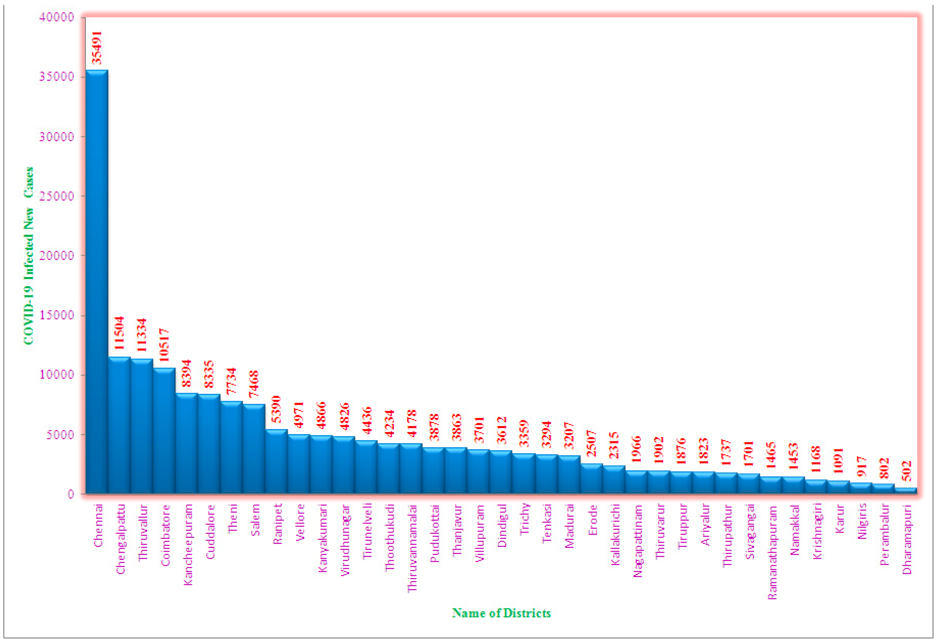
Figure 2. Total number of COVID-19-related deaths in August, 2020.

3.3. Differences between Districts

ANOVA tests were performed separately for NCASE and DEATH to assess the differences across districts in terms of number of COVID-19-positive patients and COVID-19-related fatalities. The findings are revealed in Table 2 and Table 3.

Table 2. Analysis findings for the mean equality of COVID-19 infections.

Method	df	Value	Probability
ANOVA F-test	(36, 1110)	364.6168	0.0000
Welch F-test*	(36, 389.769)	191.3449	0.0000
Analysis of Variance
Between	36	41239909	1145553.00
Within	1110	3487398	3141.80
Total	1146	44727306	39029.06

Table 2. Analysis findings for the mean equality of COVID-19 infections.

Method	df	Value	Probability
ANOVA F-test	(36, 1110)	364.6168	0.0000
Welch F-test*	(36, 389.769)	191.3449	0.0000
Analysis of Variance
Between	36	41239909	1145553.00
Within	1110	3487398	3141.80
Total	1146	44727306	39029.06

Table 3. Finding of a test for mean equality of COVID-19-related deaths.

Method	df	Value	Probability
ANOVA F-test	(36, 1110)	105.9176	0.0000
Welch F-test*	(36, 390.212)	44.55014	0.0000
Analysis of Variance
Between	36	14006.17	389.0602
Within	1110	4077.290	3.6732
Total	1146	18083.46	15.77963

Table 3. Finding of a test for mean equality of COVID-19-related deaths.

Method	df	Value	Probability
ANOVA F-test	(36, 1110)	105.9176	0.0000
Welch F-test*	(36, 390.212)	44.55014	0.0000
Analysis of Variance
Between	36	14006.17	389.0602
Within	1110	4077.290	3.6732
Total	1146	18083.46	15.77963

The findings show that highly significant differences exist between the districts as the tests of ANOVA are highly significant (p < 0.0000) for research variables. This indicates that there are considerable disparities in the number of positive infections reported in various areas, as well as the number of deaths.

3.4. A Model with Constant Coefficients or Pooled OLS Regression

NCASE and the DEATH are the dependent & independent variables, respectively, in a panel least squares analysis. Table 4 displays the regression findings on the basis of EViews, Version 11.

Table 4. Findings from a model with constant coefficients or pooled OLS regression.

Variable	Coefficient	Std Error	t-Statistic	Prob.
C	0.293996	0.082975	3.543191	0.0004
NCASE	0.016774	0.000328	51.19073	0.0000
Durbin-Watson stat	1.498142	Prob. (F-Statistic)		0.0000
Hannan-Quinn criterion	4.412060	F-Statistic		2620.491
Schwarz criterion	4.417535	Log likelihood		-2526.412
Akaike info criterion	4.408739	Sum squared resid.		5498.767
SD dependent var.	3.972358	SE of regression		2.191442
Mean dependent var.	2.952921	Adjusted R-squared		0.695657
Root MSE	2.189530	R-squared		0.695923

Table 4. Findings from a model with constant coefficients or pooled OLS regression.

Variable	Coefficient	Std Error	t-Statistic	Prob.
C	0.293996	0.082975	3.543191	0.0004
NCASE	0.016774	0.000328	51.19073	0.0000
Durbin-Watson stat	1.498142	Prob. (F-Statistic)		0.0000
Hannan-Quinn criterion	4.412060	F-Statistic		2620.491
Schwarz criterion	4.417535	Log likelihood		-2526.412
Akaike info criterion	4.408739	Sum squared resid.		5498.767
SD dependent var.	3.972358	SE of regression		2.191442
Mean dependent var.	2.952921	Adjusted R-squared		0.695657
Root MSE	2.189530	R-squared		0.695923

According to the findings, the slopes and intercept are extremely highly significant as wll as model “F-statistic” is also quite significant, with an extraordinarily high R² of 70%. This demonstrates that there is a direct correlation between growth in the cases of COVID-19 and variation in COVID-19-related deaths. Additionally, as previously mentioned, the DEATH rate rises by 0.02 percent for every unit increase in NCASE.

The main issue with this model is that it does not differentiate between the various districts or inform us as to whether the overall COVID-19 mortality response to explanatory variable over time is consistent across all districts. As a result, there is a good chance that the error term and the model’s regressor will be associated. If this is the case, the calculated coefficients in the aforementioned model could be biased and inconsistent.

3.5. FE LSDV Model

The dummy variable approach is applied to create this FE model. The model is expressed as

$$Y_{it}={\alpha }_1+{\alpha }_2{D}_{2i}+{\alpha }_{3i}{D}_{3i}+{\alpha }_4{D}_{4i}+\dots +{\alpha }_{37}{D}_{37i}+{\beta }_2{X}_{it}+{\nu }_{it}$$

where $D_{2i}=1$if the observation from Chengalpattu region and 0 otherwise, $D_{3i}=1$ if it is from Chennai and 0 otherwise,$D_{4i}=1$if it is from Coimbatore and 0 otherwise, and so on. The baseline or reference category in this case is the district of Ariyalur.As a result, the intercept${\alpha }_1$shows the value of intercept for the Ariyalur region while the other coefficients of α show how much the “intercept values” for the other regions deviate from the Ariyalur district’s intercept value. Therefore,${\alpha }_2$indicates how much the intercept 2^nd district value, Chengalpattu, differs from${\alpha }_1$. The sum $({\alpha }_2+{\alpha }_2)$provides the intercept’s actual value for Chengalpattu. Similar calculations may be made for the intercept values of the remaining districts.

The findings shown in Table 6 demonstrate that FE model is extremely significant, with an impressive R² of 77%. It is also discovered that slope coefficient for COVID-19 infections is extremely significant, demonstrating that COVID-19 infections display considerable fluctuations in the link to COVID-19-related deaths. There are several negative dummy variable coefficients discovered, but none of them are significant. The dummy variables for Nagapattinam, Karur, Kanyakumari, Erode, Dharmapuri, Cuddalore, Coimbatore, Chennai, Chengalpattu, Ramanathapuram, Salem, Sivaganga, Tenkasi, Thanjavur, Theni, Thiruvannamalai, Thiruvarur, Tirunelveli, Tiruppur, Trichy, Vellore, Virudhunagar and Villupuram are discovered to be quite highly significant, indicating that it’s possible that these district changes are heterogeneous and that the results from the combined regression model may not be useful. Moreover, the slope coefficient values in Table 5 are also different, which raises additional questions about the outcomes in Table 4. Furthermore, there is no autocorrelation in the FE model if the value of Durbin-Watson d is closer to 2. Therefore, it would appear that the FE model is superior to pooled regression paradigm.

Table 5. Regression model FE or LSDV results.

	Coefficient	Std Error	t-Statistic	Prob
C(1)	0.397195	0.256785	1.546802	0.1222
C(2)	0.005136	0.001006	5.103878	0.0000
C(3)	2.728933	0.504221	5.412180	0.0000
C(4)	15.10930	1.141332	13.23830	0.0000
C(5)	5.924730	0.486907	12.16810	0.0000
C(6)	1.157239	0.454344	2.547056	0.0110
C(7)	-0.190050	0.423176	-0.449104	0.6534
C(8)	1.455935	0.417680	3.485765	0.0005
C(9)	0.348703	0.416850	0.836520	0.4030
C(10)	0.832129	0.417020	1.995417	0.0462
C(11)	2.341012	0.455110	5.143838	0.0000
C(12)	3.151382	0.422328	7.461933	0.0000
C(13)	-0.061837	0.420283	-0.147132	0.8831
C(14)	-0.171370	0.419968	-0.408054	0.6833
C(15)	2.974654	0.417018	7.133154	0.0000
C(16)	0.341569	0.417568	0.817996	0.4135
C(17)	0.394311	0.418929	0.941237	0.3468
C(18)	-0.258813	0.421050	-0.614685	0.5389
C(19)	-0.078468	0.421597	-0.186121	0.8524
C(20)	1.315087	0.418339	3.143588	0.0017
C(21)	0.779420	0.418889	1.860682	0.0631
C(22)	1.419398	0.425410	3.336537	0.0009
C(23)	2.107346	0.443887	4.747482	0.0000
C(24)	1.385478	0.418189	3.313044	0.0010
C(25)	1.669916	0.417125	4.003391	0.0001
C(26)	1.769185	0.418298	4.229489	0.0000
C(27)	0.869724	0.446933	1.945983	0.0519
C(28)	0.766609	0.418094	1.833581	0.0670
C(29)	3.305488	0.501135	6.596002	0.0000
C(30)	2.071831	0.419295	4.941222	0.0000
C(31)	0.352173	0.417702	0.843121	0.3993
C(32)	0.933520	0.419498	2.225323	0.0263
C(33)	3.319404	0.420296	7.897779	0.0000
C(34)	1.033901	0.417759	2.474873	0.0135
C(35)	1.013985	0.417218	2.430347	0.0152
C(36)	2.263017	0.422893	5.351281	0.0000
C(37)	2.061236	0.422120	4.883059	0.0000
Durbin-Watson stat	1.914845	Prob(F-statistic)		0.000000
Hannan-Quinn criter	4.209112	F-statistic		109.0998
Schwarz criterion	4.310412	Log likelihood		-2341.690
Akaike info criterion	4.147673	Sum squared resid		3984.570
SD dependent var	3.972358	SE of regression		1.894651
Mean dependent var	2.952921	Adjusted R-squared		0.772510
Root MSE	1.863842	R-squared		0.779657”

Table 5. Regression model FE or LSDV results.

	Coefficient	Std Error	t-Statistic	Prob
C(1)	0.397195	0.256785	1.546802	0.1222
C(2)	0.005136	0.001006	5.103878	0.0000
C(3)	2.728933	0.504221	5.412180	0.0000
C(4)	15.10930	1.141332	13.23830	0.0000
C(5)	5.924730	0.486907	12.16810	0.0000
C(6)	1.157239	0.454344	2.547056	0.0110
C(7)	-0.190050	0.423176	-0.449104	0.6534
C(8)	1.455935	0.417680	3.485765	0.0005
C(9)	0.348703	0.416850	0.836520	0.4030
C(10)	0.832129	0.417020	1.995417	0.0462
C(11)	2.341012	0.455110	5.143838	0.0000
C(12)	3.151382	0.422328	7.461933	0.0000
C(13)	-0.061837	0.420283	-0.147132	0.8831
C(14)	-0.171370	0.419968	-0.408054	0.6833
C(15)	2.974654	0.417018	7.133154	0.0000
C(16)	0.341569	0.417568	0.817996	0.4135
C(17)	0.394311	0.418929	0.941237	0.3468
C(18)	-0.258813	0.421050	-0.614685	0.5389
C(19)	-0.078468	0.421597	-0.186121	0.8524
C(20)	1.315087	0.418339	3.143588	0.0017
C(21)	0.779420	0.418889	1.860682	0.0631
C(22)	1.419398	0.425410	3.336537	0.0009
C(23)	2.107346	0.443887	4.747482	0.0000
C(24)	1.385478	0.418189	3.313044	0.0010
C(25)	1.669916	0.417125	4.003391	0.0001
C(26)	1.769185	0.418298	4.229489	0.0000
C(27)	0.869724	0.446933	1.945983	0.0519
C(28)	0.766609	0.418094	1.833581	0.0670
C(29)	3.305488	0.501135	6.596002	0.0000
C(30)	2.071831	0.419295	4.941222	0.0000
C(31)	0.352173	0.417702	0.843121	0.3993
C(32)	0.933520	0.419498	2.225323	0.0263
C(33)	3.319404	0.420296	7.897779	0.0000
C(34)	1.033901	0.417759	2.474873	0.0135
C(35)	1.013985	0.417218	2.430347	0.0152
C(36)	2.263017	0.422893	5.351281	0.0000
C(37)	2.061236	0.422120	4.883059	0.0000
Durbin-Watson stat	1.914845	Prob(F-statistic)		0.000000
Hannan-Quinn criter	4.209112	F-statistic		109.0998
Schwarz criterion	4.310412	Log likelihood		-2341.690
Akaike info criterion	4.147673	Sum squared resid		3984.570
SD dependent var	3.972358	SE of regression		1.894651
Mean dependent var	2.952921	Adjusted R-squared		0.772510
Root MSE	1.863842	R-squared		0.779657”

3.6. Wald Test

We use the Wald test to examine whether pooled OLS or FE model is more appropriate. The null hypothesis in this situation is that OLS regression model is suitable (all dummy variables equivalent 0), as well as alternative hypothesis is the model of FE is suitable (all dummy variables don’t equivalent 0). Thus, this test is performed and the findings are expressed in Table 6.

Table 6. Findings of Wald test.

Test Statistic	Value	df	Probability
F-Statistic	12.05191	(35, 1110)	0.0000
Chi-square	421.8168	35	0.0000

Table 6. Findings of Wald test.

Test Statistic	Value	df	Probability
F-Statistic	12.05191	(35, 1110)	0.0000
Chi-square	421.8168	35	0.0000

The FE or LSDV regression model is shown to be more suitable as compared to panel pooled regression model by the Wald test F-statistic, which is determined to be highly significant (p < 0.0000). Not every dummy variable has a value of zero.

3.7. RE Mode

Table 7 displays the test results for the RE model, which keeps the number of COVID-19-related deaths as the dependent variable as well as NCASE as independent variable.

Table 7. Fitted RE model results.

Variable	Coefficient	Std. Error	t-Statistic	Prob.
C	0.943137	0.188271	5.009478	0.0000
NCASE	0.012679	0.000644	19.675290	0.0000
Effects Specification
Cross-section random			0.899741	0.1839
Idiosyncratic random			1.895478	0.8161
Weighted Statistics
Root MSE	1.967594	R-squared		0.238511
Mean dependent var	1.045002	Adjusted R-squared		0.237846
S.D. dependent var	2.255761	S.E. of regression		1.966931
Sum squared resid	4440.525	F-statistic		358.6336
Durbin-Waston stat	1.784844	Prob (F-statistic)		0.000000
Unweighted Statistics
Sum squared resid	6248.849	Durbin-watson stat.		1.268337
R-squared	0.654444	Mean dependent var		2.952921

Table 7. Fitted RE model results.

Variable	Coefficient	Std. Error	t-Statistic	Prob.
C	0.943137	0.188271	5.009478	0.0000
NCASE	0.012679	0.000644	19.675290	0.0000
Effects Specification
Cross-section random			0.899741	0.1839
Idiosyncratic random			1.895478	0.8161
Weighted Statistics
Root MSE	1.967594	R-squared		0.238511
Mean dependent var	1.045002	Adjusted R-squared		0.237846
S.D. dependent var	2.255761	S.E. of regression		1.966931
Sum squared resid	4440.525	F-statistic		358.6336
Durbin-Waston stat	1.784844	Prob (F-statistic)		0.000000
Unweighted Statistics
Sum squared resid	6248.849	Durbin-watson stat.		1.268337
R-squared	0.654444	Mean dependent var		2.952921

The findings are revealed in Table 8, and the model coefficients are shown to be extremely significant. The RE model only explains 24 percent of the variance in DEATH in proportion to the NCASE. The cross-sectional effects individually amount to 0.2 percent according to the rho value of 0.1839.

Table 8. Results of Hausman test (Test cross-section REs).

Test Summary		Chi-Sq. Statistic	Chi-Sq. d.f.	Prob.
Cross-section random		91.938632	1	0.0000
Cross-section random effects test comparisons:
Variable	Fixed	Random	Var(Diff.)	Prob.
NCASE	0.005159	0.012679	0.000001	0.0000
Cross-section random effects test equation:
Variable	Coefficient	Std. Error	t-Statistic	Prob.
C	2.135067	0.170350	12.53341	0.0000
NCASE	0.005159	0.001015	5.083191	0.0000
Effects Specification
Durbin-Watson stat	1.914989	Prob(F-statistic)		0.000000
Hannan-Quinn criter	4.212487	F-statistic		106.0594
Schwarz criterion	4.316525	Log likelihood		-2341.674
Akaike info criterion	4.149388	Sum squared resid		3984.456
S.D. dependent var	3.972358	S.E. of regression		1.895478
Mean dependent var	2.952921	Adjusted R-squared		0.772312
Root MSE	1.863815	R-squared		0.779663”

Table 8. Results of Hausman test (Test cross-section REs).

Test Summary		Chi-Sq. Statistic	Chi-Sq. d.f.	Prob.
Cross-section random		91.938632	1	0.0000
Cross-section random effects test comparisons:
Variable	Fixed	Random	Var(Diff.)	Prob.
NCASE	0.005159	0.012679	0.000001	0.0000
Cross-section random effects test equation:
Variable	Coefficient	Std. Error	t-Statistic	Prob.
C	2.135067	0.170350	12.53341	0.0000
NCASE	0.005159	0.001015	5.083191	0.0000
Effects Specification
Durbin-Watson stat	1.914989	Prob(F-statistic)		0.000000
Hannan-Quinn criter	4.212487	F-statistic		106.0594
Schwarz criterion	4.316525	Log likelihood		-2341.674
Akaike info criterion	4.149388	Sum squared resid		3984.456
S.D. dependent var	3.972358	S.E. of regression		1.895478
Mean dependent var	2.952921	Adjusted R-squared		0.772312
Root MSE	1.863815	R-squared		0.779663”

3.8. Hausman Test

The RE model performs better. The FE and RE estimators are compared using the Hausman test to observe if there is a significant variation. The statistic of Hausman test is significant, and null hypothesis is rejected, according to the findings shown in Table 9, demonstrating the suitability of the FE model. The Hausman test yields an R² value of 80%, which is exceptionally high. The conclusion that the RE model is suitable is refuted by this observation. Additionally, the regressor variable’s RE and FE coefficient values are shown to be highly statistically significant in the final row of Table 8.

4. Conclusions

For analysing trends and the link between new COVID-19 infections and COVID-19-related mortality, a pooled regression model was not appropriate. ANOVA test results show significant variation across districts. The greatest number of fresh cases of COVID-19 has been noted in Chennai (35,491), followed by Coimbatore (11,504), Thiruvallur (11,334), Chengalpattu (10,517), and Tirunelveli (8,393). The least numbers of fresh cases of COVID-19 were reported in Krishnagiri (917), Dharmapuri (802) and Nilgiris (502). Overall, in August 2020, 181,817 COVID-19-infected patients were registered across Tamil Nadu. The greatest DEATH because of COVID-19 was in Chennai (663), followed by Coimbatore (250), Thiruvallur (138), Chengalpattu (156), Tirunelveli (138), and Kanyakumari (135). Nine deaths were registered in Dharmapuri and Nilgiris, which is the lowest figure among the districts. In total, in August 2020, 3,387 deaths have been reported because of COVID-19 in Tamil Nadu, India. The fixed effect model, which has the greatest R² value of 77%, is quite important. The slope coefficient is also found to be highly significant, showing that significant variation exists in the relationship between fresh COVID-19 cases and deaths because of COVID-19. Additionally, for every unit increase in COVID-19-infected cases, the death rate increased by 0.02%.

References

- Voyages, A. The Importance of Statistical Modeling for the COVID-19 Pandemic. Young Scientist Journal 2021. [Google Scholar]
- Santosh, K. C. AI-Driven Tools for Coronavirus Outbreak: Need of Active Learning and Cross-Population Train/Test Models on Multitudinal/Multimodal Data. J. Med. Syst. 2020, 44(5). [Google Scholar] [CrossRef]
- Al-Rousan, N.; Al-Najjar, H. Data Analysis of Coronavirus COVID-19 Epidemic in South Korea Based on Recovered and Death Cases. J. Med. Virol. 2020, 92(9), 1603–1608. [Google Scholar] [CrossRef]
- Gondauri, D.; Mikautadze, E.; Batiashvili, M. Research on COVID-19 Virus Spreading Statistics Based on the Examples of the Cases from Different Countries. Electron. J. Gen. Med. 2020, 17(4), em209. [Google Scholar] [CrossRef]
- Gondauri, D.; Batiashvili, M. The Study of the Effects of Mobility Trends on the Statistical Models of the COVID-19 Virus Spreading. Electron. J. Gen. Med. 2020, 17(6), em243. [Google Scholar] [CrossRef]
- Katris, C. A Time Series-Based Statistical Approach for Out Break Spread Forecasting: Application of COVID-19 in Greece. Expert Systems with Applications 2021, 166. [Google Scholar] [CrossRef]
- Kumar, A. Application of Mathematical Modeling in Public Health Decision Making Pertaining to Control of COVID-19 Pandemic in India. Epidemiology International 2020, 5, 23–26. [Google Scholar]
- Mittal, S.; International Institute of Information Technology-Banglore. An Exploratory Data Analysis of COVID-19 in India. Int. J. Eng. Res. Technol. (Ahmedabad) 2020, V9(04). [Google Scholar] [CrossRef]
- Ogundokun, R. O.; Lukman, A. F.; Kibria, G. B. M.; Awotunde, J. B.; Aladeitan, B. B. Predictive Modelling of COVID-19 Confirmed Cases in Nigeria. Infect. Dis. Model. 2020, 5, 543–548. [Google Scholar] [CrossRef]
- Takele, R. Stochastic Modelling for Predicting COVID-19 Prevalence in East Africa Countries. Infect. Dis. Model. 2020, 5, 598–607. [Google Scholar] [CrossRef]
- Rajarathinam, A.; Tamilselvan, P. Autoregressive Distributed Lag Model of COVID-19 Cases and Deaths. Appl. Math. Inf. Sci 2021. [Google Scholar]
- Rajarathinam, A.; Tamilselvan, P. Vector Error Correction Modeling of Covid-9 Infected Cases and Deaths. Journal of Statistics Applications & Probability 2021. [Google Scholar]
- Hsiao, C. Analysis of Panel Data; Cambridge University Press, 2003. [Google Scholar]
- Baltagi, B. H. Econometric Analysis of Panel Data, 4th ed.; Standards Information Network; 2012. [Google Scholar]
- Allison, P. D. Fixed Effects Regression Models; SAGE Publications: Thousand Oaks, CA, 2009. [Google Scholar]
- Biorn, E. Econometrics of Panel Data: Methods and Applications; Oxford University Press: London, England, 2016. [Google Scholar]
- Gujarati, D. N.; Porter, D. C. Basic Econometrics, 6th ed.; McGraw-Hill Education: Singapore, Singapore, 2017. [Google Scholar]
- Hadri, K. Testing for Stationarity in Heterogeneous Panel Data. Econom. J. 2000, 3, 148–161. [Google Scholar] [CrossRef]
- Levin, A.; Lin, C.-F.; James Chu, C.-S. Unit Root Tests in Panel Data: Asymptotic and Finite-Sample Properties. J. Econom. 2002, 108, 1–24. [Google Scholar] [CrossRef]
- Hausman, J. A. Specification Tests in Econometrics. Econometrica 1978, 46. [Google Scholar] [CrossRef]
- Wald, A. Tests of Statistical Hypotheses Concerning Several Parameters When the Number of Observations Is Large, Transactions of The; American Mathematical Society, 1943; Vol. 54. [Google Scholar]
Disclaimer/Publisher’s Note: The statements, opinions and data contained in all publications are solely those of the individual author(s) and contributor(s) and not of MDPI and/or the editor(s). MDPI and/or the editor(s) disclaim responsibility for any injury to people or property resulting from any ideas, methods, instructions or products referred to in the content. |
© 2023 by the authors. Licensee MDPI, Basel, Switzerland. This article is an open access article distributed under the terms and conditions of the Creative Commons Attribution (CC BY) license (http://creativecommons.org/licenses/by/4.0/).
Copyright: This open access article is published under a Creative Commons CC BY 4.0 license, which permit the free download, distribution, and reuse, provided that the author and preprint are cited in any reuse.