Submitted:
08 August 2023
Posted:
09 August 2023
You are already at the latest version
Abstract
The Chen circuit system, a three-dimensional autonomous system with intriguing dynamics, has gained considerable attention due to its potential applications in diverse scientific fields. In this article, a Chen circuit-like system is defined and a comprehensive dynamics has been studied. The system exhibits chaotic dynamics, limit cycles, and bifurcations, making it a captivating subject of study. By employing numerical simulations and analytical techniques, we explore the system's stability and identify critical parameter values leading to qualitative changes. Notably, we delve Hopf bifurcations, which give rise to stability changes and the emergence of limit cycles. Furthermore, we analyze the fractal dimension of the system's attractor, providing insights into its complexity and self-similarity. Through a systematic examination of the Chen circuit-like system, we deepen our understanding of its intricate dynamics and offer valuable insights into the underlying mechanisms. The findings contribute to the field of dynamical systems and hold potential implications in areas such as chaos-based secure communications, signal processing, and nonlinear control. This work serves as a valuable reference for researchers and practitioners interested in the dynamics and bifurcation analysis of nonlinear systems.
Keywords:
Chen-like chaotic system
; limit cycle
; chaotic solution
; local asymptotic stability
; bifurcation
; phase portrait analysis
MSC: 54A40; 22A05; 54E15; 03E72; 08A72
1. Introduction
The exploration of dynamical systems plays a pivotal role in understanding complex phenomena across diverse scientific disciplines, ranging from physics and biology to engineering and economics. Most of the complex dynamical chaotic and hyper-chaotic system of nonlinear ODEs characterizes phenomenons. For instance, variations in population dynamics can be discussed and predictions can be made for the future scenarios. Moreover, Lorenz introduced a model in 1963 for weather forecasting [1], demonstrating temperature and wind speed variations. He observed that small perturbations in the initial conditions of the proposed dynamical model led to surprising results. This effect is known as the butterfly effect, as the system has sensitive dependence on the initial conditions.
The world chaos was used by Li and Yorke in 1975 for the first time in their research [2]. In 1976, Rossler considered a prototype equation to the Lorenz model that behaves similarly to the Lorenz model but in low dimensional dissipative dynamical systems [3]. He also proposed an even simpler (algebraic) model in 1979 [4]. Matsumoto et al. developed an autonomous chaotic system 1986 concerning the basic circuit layout. This circuit is known in the literature as the “Chua circuit” [5]. Chen and Ueta discovered a chaotic system in 1999, known as the Chen system [6] based on the Lorenz model. Another chaotic system has been investigated in [7] by Lu and Chen, representing the transition between the Lorenz and Chen systems. Sprott studied generic three-dimensional systems with quadratic nonlinearities [8,9,10]. He found nineteen different chaotic systems by exhaustive computer research such that there is no apparent transformation of one to another. Many other chaotic systems have been introduced and analyzed in the literature, including the Liu system [11,12].
Thus chaos is a highly complex nonlinear dynamical phenomenon in nature. Much research has been reported in the literature investigating various characteristics associated with dynamical systems. Edward Lorenz discovered a strange attractor while finding the numerical solutions to the proposed weather model [13]. In recent years, motivated by different applications, great works have been reported in constructing the chaotic and hyper-chaotic dynamical models [17,18,19,20,21,22,23,24,25,26,27,28,29,30,31,32].
Among the intriguing dynamical systems, the Chen circuit system has garnered significant attention due to its remarkable dynamics and potential applications in various domains. In this study, a Chen circuit-like system is defined as follows:
The Chen circuit-like system exhibits a rich variety of behaviors, including chaotic dynamics, bifurcations, and limit cycles. Its dynamics are governed by a set of nonlinear ordinary differential equations, capturing the interactions among its state variables. Specifically, the system involves variables and z, coupled through nonlinear terms incorporating parameters and d.
In this article, we embark on a comprehensive analysis of the Chen circuit-like system, aiming to unveil its intricate dynamics and investigate its bifurcation behavior. Our objective is to comprehend the system’s stability, explore the critical parameter values triggering qualitative changes, and elucidate the underlying mechanisms governing its observed dynamics. To achieve this, we employ a combination of numerical simulations and analytical techniques to study the system’s behavior under parameter variations. Our focus lies on conducting bifurcation analyses to identify the specific parameter values at which significant changes in the system’s dynamics occur. Notably, we delve into the exploration of Hopf bifurcations, which lead to stability changes and the emergence of limit cycles. Furthermore, we delve into the fractal dimension analysis of the attractor generated by the Chen circuit-like system. The fractal dimension provides valuable insights into the complexity and self-similarity of the attractor, shedding light on the underlying dynamical properties of the system. By employing the box-counting method, we estimate the fractal dimension and discuss its implications in relation to the system’s chaotic behavior.
Through our in-depth analysis, we aim to deepen the understanding of the Chen circuit-like system’s complex dynamics and provide valuable insights into the underlying mechanisms governing its behavior. The findings presented in this article contribute to the broader field of dynamical systems and offer potential applications in diverse areas such as chaos-based secure communications, signal processing, and nonlinear control.
The subsequent sections of the article are structured as follows: Section 2 provides a concise overview of the Chen circuit-like system and presents a comprehensive stability analysis of the system and identify critical parameter ranges associated with distinct dynamical regimes. Section 3 and 4 focus on limit cycles and chaotic solutions of the system, respectively. Bifurcation analysis is presented in the Section 5. Finally, Section 6 summarizes the key findings and offers concluding remarks.
We believe that this thorough investigation of the Chen circuit-like system contributes to the growing body of knowledge on nonlinear dynamical systems and serves as an essential reference for researchers and practitioners working in the field.
2. Chen-like system and its dynamical analysis
In this present study, we have introduced the new chaotic system:
where x, y and y are state variables and and d are parameters.
2.1. Symmetry and Invariance
It is simple to see the invariance of system 2.1 under the coordinate transformation
That is, the system 2.1 has symmetry around the z-axis [15]. Hence, we can observe that the variables x and y are symmetrical with respect to the origin .
2.2. Dissipativity
The proposed dynamical system 2.1 can be written in the vector form as
The divergence of the vector field on is given by
For the system 2.1, the divergence is computed as , which is negative if , so that decreases at rate
Solving the above differential equation, we have
So the volume of the system reduces exponentially fast to 0 , and hence the dynamical model 2.1 is a dissipative system for . That is, every volume consisting of the system trajectory shrinks to zero as at an exponential rate of . Thus, all the system orbits are confined to a specific subset containing zero volume and the asymptotic motion converges onto an attractor [16,26].
2.3. System equilibria
Definition 2.1.
[30] The steady-state equilibrium, , is hyperbolic if none of the eigenvalues of lies on the unit circle, i. e., if , for .
Definition 2.2.
[30] Consider the discrete, nonlinear dynamical system in 2.1 with a steady-state equilibrium, . The associated Jacobian matrix has three eigenvalues .
(i) The steady-state equilibrium is called a sink if for all .
(ii) The steady-state equilibrium is called a two-dimensional saddle if one .
(iii) The steady-state equilibrium is called a one-dimensional saddle if one .
(iv) The steady-state equilibrium is called a source if for all .
Resule 2.3.
Routh–Hurwitz stability criterion states that the equilibrium of a three dimensional system is locally asymptotically stable if and only if,are positive and, where,andare the coefficient of the characteristic polynomialof the Jacobian at the equilibrium.
Lemma 2.4.
[31] We consider a cubic polynomial equation of the following type:
where , and represents real constants. Furthermore, all roots for the polynomial equation 2.6 lie within the open disk if and only if the following conditions are satisfied:
The equilibria of the chaotic system 2.1 are found by setting ,
i. e.,
The system 2.1 has three equilibrium points:
, , and
Since the equilibrium points and are reflection of each other with respect to z-axis, we only would be interested to explore dynamical behavior of without loss of generality.
The local behavior of the system around these equilibrium points can be investigated by using the following Jacobian matrix:
Dynamical behavior about :
For the equilibrium point , the above Jacobian matrix becomes the following
To obtain its eigenvalues, let . Then, the characteristic equation has the following form:
Solving the above characteristic equation, the eigenvalues are found as
Lemma 2.5.
(i) is a sink if and only if , and .
(ii) is a source if and only if , and .
(iii) is a saddle node if and only if , and .
(iv) is non-hyperbolic if and only if , and .
Here we present four examples which illustrate Lemma 2.5.
Example 2.6.
Consider the parameters and satisfying the conditions , and . then the equilibrium is a sink. (Figure 1).
Example 2.7.
Consider the parameters and satisfying the conditions , and . then the equilibrium is a source (Figure 2).
Example 2.8.
Consider the parameters and satisfying the conditions , and , then the equilibrium is a saddle node. (Figure 3).
Example 2.9.
Consider the parameters , and , then the of system 2.1 is non-hyperbolic. (Figure 4).
Dynamical behavior about :
For the equilibrium point , the above Jacobian matrix becomes the following
To obtain its eigenvalues, let . Then, the characteristic equation has the following form:
Comparing equation 2.9 and equation 2.6, we have
Lemma 2.10.
The steady state for model 2.1 is a sink and it is locally asymptotically stable if and only if the following inequalities are satisfied:
where and are written in 2.10.
Example 2.11.
By satisfying the Lemma 2.10, consider the parameters be , , , and , then the system 2.1 converges to (Figure 5).
Following examples (2.11–2.12) are presented where the condition stated in the Lemma 2.10 do not satisfy.
Example 2.12.
Consider the parameters be , , , and , then the system 2.1 forms chaotic trajectory (Figure 6).
3. Limit Cycles
Here we present a set of examples depicting limit cycles with very high periodicities.
Example 3.1.
Consider the parameters be , , , and , then the system 2.1(with the initial value forms a limit cycle of period 69. (Figure 7).
Example 3.2.
Consider the parameters be , , , and , then the system 2.1(with the initial value forms a limit cycle of period 425. (Figure 8).
Example 3.3.
Consider the parameters be , , , and , then the system 2.1(with the initial value forms a limit cycle of period 689. (Figure 9).
4. Chaotic Solutions
Here we have listed parameters and d for which the dynamical system 2.1 possesses chaotic trajectories with positive Lyapunov exponent (Table 1, Table 2 and Table 3). For each set of parameters, Lyapunov exponent were calculated and the same is plotted in Figure 10. In addition, box plot of range of values from the interval for each parameter is figured in Figure 10.
Example 4.1.
Consider the parameters be a=0.2575, b=0.8407, c=0.2543, and d=0.8143, then the system 2.1(with the initial value forms a chaotic trajectory (Figure 11).
Here fractal dimension of the three dimensional chaotic attractor is turned out to be 1.9645. Non-zero fractal dimension reconfirms the chaotic behaviour of the three dimensional attractor.
Example 4.2.
Consider the parameters be a=388, b=244, c=218, and d=224, then the system 2.1(with the initial value forms a chaotic trajectory (Figure 12).
Here fractal dimension of the three dimensional chaotic attractor is turned out to be 0.73486. Non-zero fractal dimension reconfirms the chaotic behaviour of the three dimensional attractor.
Example 4.3.
Consider the parameters be a=388, b=244, c=218, and d=224, then the system 2.1(with the initial value forms a chaotic trajectory (Figure 13).
Here fractal dimension of the three dimensional chaotic attractor is turned out to be 0.50202. Non-zero fractal dimension reconfirms the chaotic behaviour of the three dimensional attractor.
5. Bifurcation Analysis
In the present system, the parameter b is the most suitable choice to observe bifurcation. This is because the equation involving b contains a non-linear term () that can lead to bifurcation behavior.
By varying the parameter b, one can observe changes in the system’s dynamics, such as stable equilibrium points, limit cycles, or chaotic behavior. Bifurcations, such as saddle-node bifurcation, pitchfork bifurcation, or Hopf bifurcation, may occur as the parameter b crosses certain critical values. Therefore, focusing on the bifurcation analysis with the parameter b will provide insights into the qualitative changes in the system’s behavior as b is varied.
5.1. Hopf Bifurcation at
The three-dimensional Hopf bifurcation theory is used to analyze the parametric variations of the system 2.1 according to its dynamical bifurcation. In this section we discussion the existence of Hopf bifurcation for the equilibrium point .
In order to see the in stability of system 2.1 let us consider b as bifurcation parameter.For this purpose let us first state the following theorem.
Theorem 5.1.
[33] If and listed in 2.10 are smooth functions of b in an open interval about such that the characteristic equation 2.9 has
(i) a pair of complex eigenvalues (with ) so that they become purely imaginary at and ,
(ii) the other eigenvalue is negative at ,
then a Hopf bifurcation occurs around at (i.e., a stability change of accompanied by the creation of a limit cycle at ).
Theorem 5.2.
System 2.1 possesses a Hopf bifurcation around when b passes through provided
where and are listed in 2.10.
Proof.
For , the characteristic equation of system 2.1 at becomes
providing roots . Thus, there exists a pair of purely imaginary eigenvalues and a strictly negative real eigenvalue. Also are smooth functions of b.
So, for b in a neighbourhood of , the roots have the form , where are real.
Next we shall verify the transversality conditions:
Substituting into the characteristic equation 2.9, we get
Now,let us take derivative of both sides of 5.1 with respect to b:
Equating real and imaginary parts from the both sides of 5.2, we get
and
where
From 5.3 and 5.4, we get
Now,
At :
Case I:
Therefore,
So, at , when .
Case II:
Therefore,
So, at , when .
Therefore,
and
Hence, by Theorem 5.1, the result follows. □
Example 5.3.
Consider the parameters and b as the bifurcation parameter ranging from to . Then exchange the stability and Hopf bifurcation takes place by Theorem 5.2. Therefore the Hopf bifurcation diagrams are presented in (Figure 14). Finally the bifurcation point and Hopf bifurcation for different set of parameters are drawn in (Figure 15).
6. Discussions and Concluding Remarks
The study of the Chen circuit-like system has provided valuable insights into the dynamics and bifurcation behavior of this intriguing three-dimensional autonomous system. Through our analysis, we have unraveled the system’s complex dynamics, explored bifurcation phenomena, and investigated the fractal properties of its attractor. This section presents a summary of the key findings and discusses their implications and potential future directions. Firstly, our analysis revealed that the Chen circuit-like system exhibits a wide range of dynamic behaviors, including chaotic dynamics, stable equilibria, and limit cycles. The system’s sensitivity to initial conditions, demonstrated by its chaotic behavior, suggests its potential applications in chaos-based secure communications and random number generation. Furthermore, the emergence of stable equilibria and limit cycles provides opportunities for designing nonlinear oscillators and exploring synchronization phenomena.
The bifurcation analysis offered valuable insights into the system’s stability and qualitative changes in its dynamics. The Hopf bifurcations unveiled the emergence of limit cycles as the system’s dynamics transitioned from stable equilibria. These findings shed light on the critical parameter values that dictate the system’s stability and the onset of complex dynamics. Moreover, the fractal dimension analysis provided a quantitative measure of the attractor’s complexity and self-similarity. The estimation of the fractal dimension using the box-counting method unveiled the system’s underlying structure and demonstrated its sensitivity to parameter changes. The observed fractal nature of the attractor highlights the intricate patterns and fine-scale details embedded within the system’s dynamics.
In conclusion, the study of the Chen circuit-like system has deepened our understanding of its intricate dynamics and provided valuable insights into the system’s stability, bifurcations, and fractal properties. The findings presented in this work contribute to the broader field of nonlinear dynamical systems and hold potential implications in various scientific disciplines, including secure communications, signal processing, and control engineering. Future research directions may include further exploration of the system’s parameter space, investigating higher-dimensional versions of the Chen circuit-like system, and analyzing the system’s response to external perturbations or feedback control strategies. Additionally, studying the synchronization behavior of multiple Chen circuit-like systems and investigating their applications in chaotic synchronization and secure communications could be fruitful avenues for future investigations.
Authorship Contribution: Both the authors contributed equally from the designing of the project to completion.
Funding: The authors do not receive any funding towards the present study.
Conflict of Interest: We declare that there is no conflict of interest.
Ethical approval: This article does not contain any studies with human participants or animals performed by any of the authors.
References
- E. N. Lorenz, (1963) ”Deterministic nonperiodic flow,” Journal of Atmospheric Sciences, vol. 20, pp. 130-141.
- T. Y. Li and J. A. Yorke, (1975) ”Period Three Implies Chaos,” The American Mathematical Monthly, vol. 82, pp. 985-992.
- O. E. Rossler, (1976) ”An equation for continuous chaos,” Physics Letters A, vol. 57, no. 5, pp. 397-398.
- O. E. Rossler, (1979) ”Continuous chaos; four prototype equations,” Annals of the New York Academy of Sciences, vol. 316, no. 1, pp. 376-392.
- T. Matsumoto, L. O. Chua, and S. Tanaka, (1984) ”Simplest chaotic nonautonomous circuit,” Physical Review A, vol. 30, pp. 1155-1157.
- G. Chen and T. Ueta, (1999) ”Yet another chaotic attractor,” International Journal of Bifurcation and Chaos, vol. 09, no. 07, pp. 1465-1466.
- J. Lu, G. Chen, and S. Zhang, (2002) ”Dynamical analysis of a new chaotic attractor.,” International Journal of Bifurcation and Chaos, vol. 12, no. 5, pp. 1001- 1015.
- J. C. Sprott, (1994) ”Some simple chaotic flows,” Physical Review-Section EStatistical Physics Plasma Fluids Related Interdiscpl Topics, vol. 50, no. 2, p. R647.
- J. C. Sprott, (1997) ”Simplest dissipative chaotic flow,” Physics letters A, vol. 228, no. 4, pp. 271-274.
- J. C. Sprott, (2000) ”A new class of chaotic circuit,” Physics Letters A, vol. 266, no. 1, pp. 19-23.
- J. C. Sprott, (2000) ”A new class of chaotic circuit,” Physics Letters A, vol. 266, no. 1, pp. 19-23.
- R. A. V. Gorder and S. R. Choudhury, (2011) ”Analytical hopf bifurcation and stability analysis of t system,” Communications in Theoretical Physics, vol. 55, no. 4, p. 609.
- I. Pehlivan and Y. Uyaroglu, (2007) ”Simplied chaotic diffusionless lorentz attractor and its application to secure communication systems,” IET Communications, vol. 1, no. 5, pp. 1015-1022.
- P. Lijun, D. Lixia, and L. Huayan, (2010) ”Dynamics of the coupled lorenz-rossler systems,” in Proceedings of the 2010 InternationalWorkshop on Chaos-Fractal Theories and Applications, IWCFTA ’ 10, (Washington, DC, USA), pp. 271- 274, IEEE Computer Society.
- S. Strogatz, (2007) Nonlinear Dynamics And Chaos. Studies in nonlinearity, Sarat Book House.
- X.-F. Li, K. E. X.-F. Li, K. E. Chlouverakis, and D.-L. Xu, (2009) ”Nonlinear dynamics and circuit realization of a new chaotic flow: A variant of lorenz, chen and l,” Nonlinear Analysis: Real World Applications, vol. 10, no. 4, pp. 2357-2368.
- Y. Uyaroglu and I. Pehlivan, (2010) ”Nonlinear sprott94 case a chaotic equation: Synchronization and masking communication applications,” Computers and Electrical Engineering, vol. 36, no. 6, pp. 1093-1100.
- Z. Wei and Q. Yang, (2011) ”Dynamical analysis of a new autonomous 3-d chaotic system only with stable equilibria,” Nonlinear Analysis: Real World Applications, vol. 12, no. 1, pp. 106-118.
- T. Wang, X. T. Wang, X. Wang, M. Wang, (2011) Chaotic control of H´enon map with feedback and nonfeedback methods, Commun. Nonlinear Sci. Numer. Simulat., 16, 3367–3374.
- A. N. Michel, L. A. N. Michel, L. Hou, D. Liu, (2007) Stability of dynamical systems: continuous, discontinuous, and discrete Systems, Boston, Birkhauser.
- E. Ott, C. E. Ott, C. Grebogi, J. A. Yorke, (1990) Controlling chaos, Phys. Rev. Letters, 64(11), 1196–1199.
- I. Pehlivan and Y. Uyaroglu, (2012) ”A new 3d chaotic system with golden proportion equilibria: Analysis and electronic circuit realization,” Computers and Electrical Engineering, vol. 38, no. 6, pp. 1777-1784.
- V. Sundarapandian and I. Pehlivan, (2012) ”Analysis, control, synchronization, and circuit design of a novel chaotic system,” Mathematical and Computer Modelling, vol. 55, no. 7-8, pp. 1904-1915.
- S. Cicek, Y. S. Cicek, Y. Uyaroglu, and I. Pehlivan, (2013) ”Simulation and circuit implementation of sprott case h chaotic system and its synchronization application for secure communication systems,” Journal of Circuits, Systems, and Computers, vol. 22, no. 4.
- S. Gang-Quan, C. S. Gang-Quan, C. Hui, and Z. Yan-Bin, (2011) ”A new four-dimensional hyperchaotic lorenz system and its adaptive control,” Chinese Physics B, vol. 20, no. 1, p. 010509.
- W. Zhou, Y. W. Zhou, Y. Xu, H. Lu, and L. Pan, (2008) ”On dynamics analysis of a new chaotic attractor,” Physics Letters A, vol. 372, no. 36, pp. 5773-5777.
- F. J. Romeiras, C. F. J. Romeiras, C. Grebogi, E. Ott, W. P. Dayawansa, (1992) Controlling chaotic dynamical systems, Physica D, 58, 165–192.
- C. Robinson, (1999) Dynamical Systems: Stability, Symbolic Dynamics and Chaos, Boca Raton, New York.
- S. Wiggins, (2003) Introduction to Applied Nonlinear Dynamical Systems and Chaos, Springer–Verlag, New York.
- A. Tabakovic, (2015) On the Characterization of Steady-States in Three-Dimensional Discrete Dynamical Systems, CREA, University of Luxembouurg.
- E. Camouzis, G. E. Camouzis, G. Ladaas, (2008) Dynamics of Three-Order Rational Difference Equations with Open Problems and Conjectures, Chapman and Hall, New York.
- G. Chen, X. G. Chen, X. Dong, (1998) From Chaos to Order: Perspectives, Methodologies, and Applications, World Scientific, Singapore.
- J.D. Murray,(1989) Mathematical Biology, Springer-Verlag,Berlin.
- G. Wen, (2005) Criterion to identify Hopf bifurcations in maps of arbitrary dimension Phys. Rev. E 72, Article ID 026201.
- G. Wen, S. G. Wen, S. Chen, Q. Jin, (2008) A new criterion of period-doubling bifurcation in maps and its application to an inertial impact shaker. J. Sound Vib. 311, 212–223.
- Y. A. Kuznetsov, (1997) Elements of Applied Bifurcation Theory, Springer-Verlag, New York.
Figure 1.
Sink trajectory in 3 dimension and two dimensional phase portraits
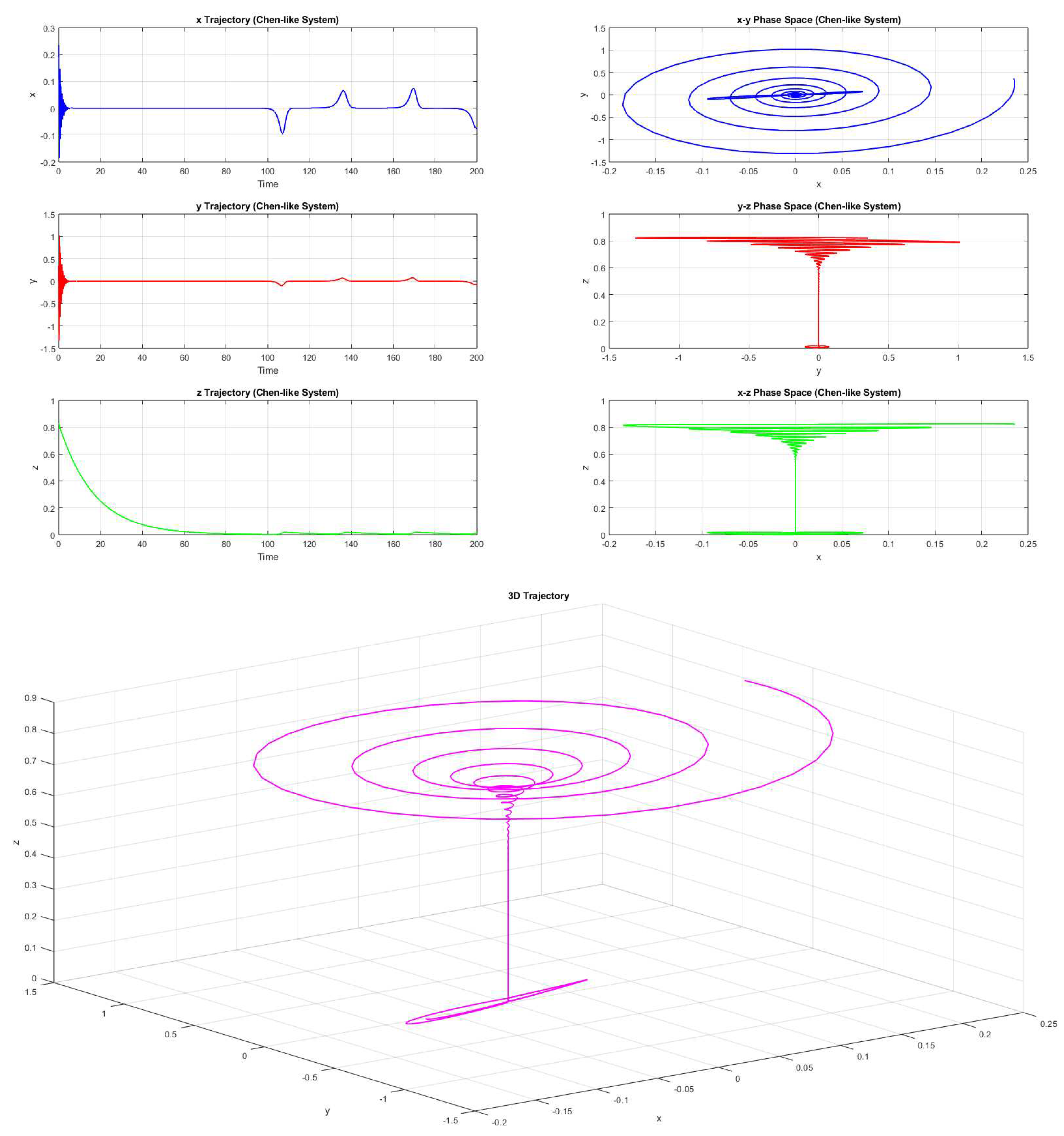
Figure 2.
Source trajectory in 3 dimension and two dimensional phase portraits
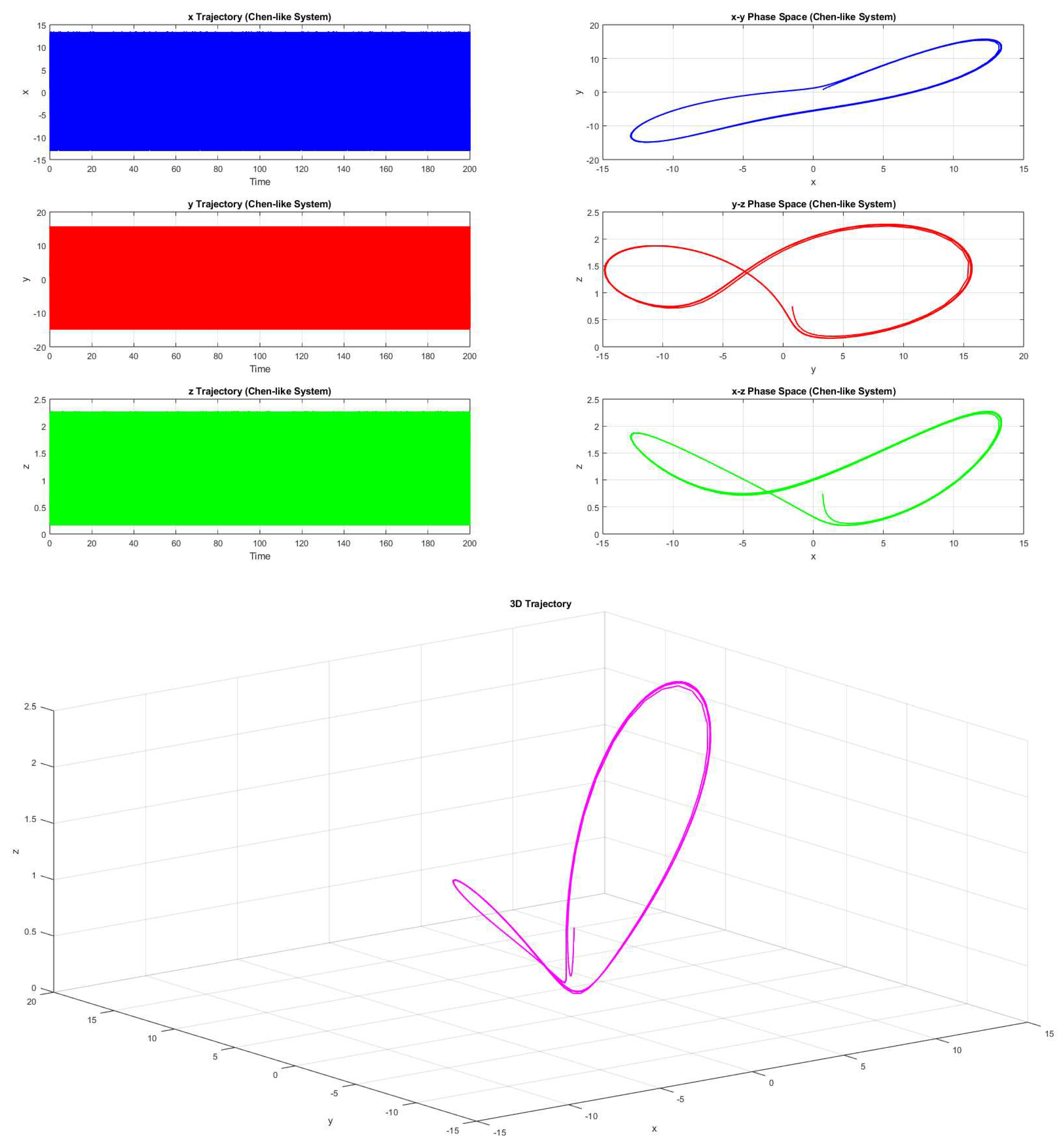
Figure 3.
Saddle node trajectory in 3 dimension and two dimensional phase portraits
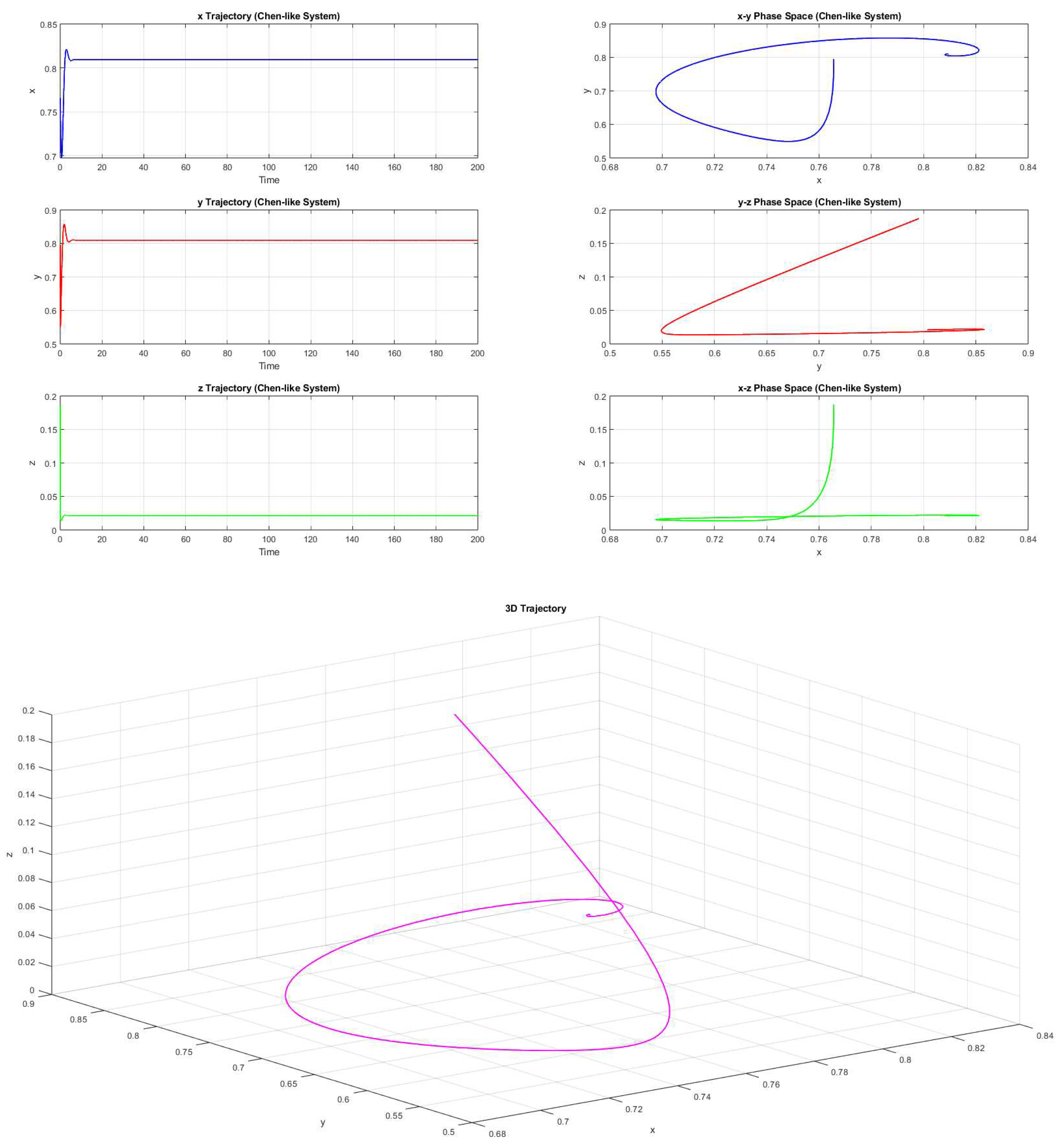
Figure 4.
Non-hyperbolic trajectory in 3 dimension and two dimensional phase portraits
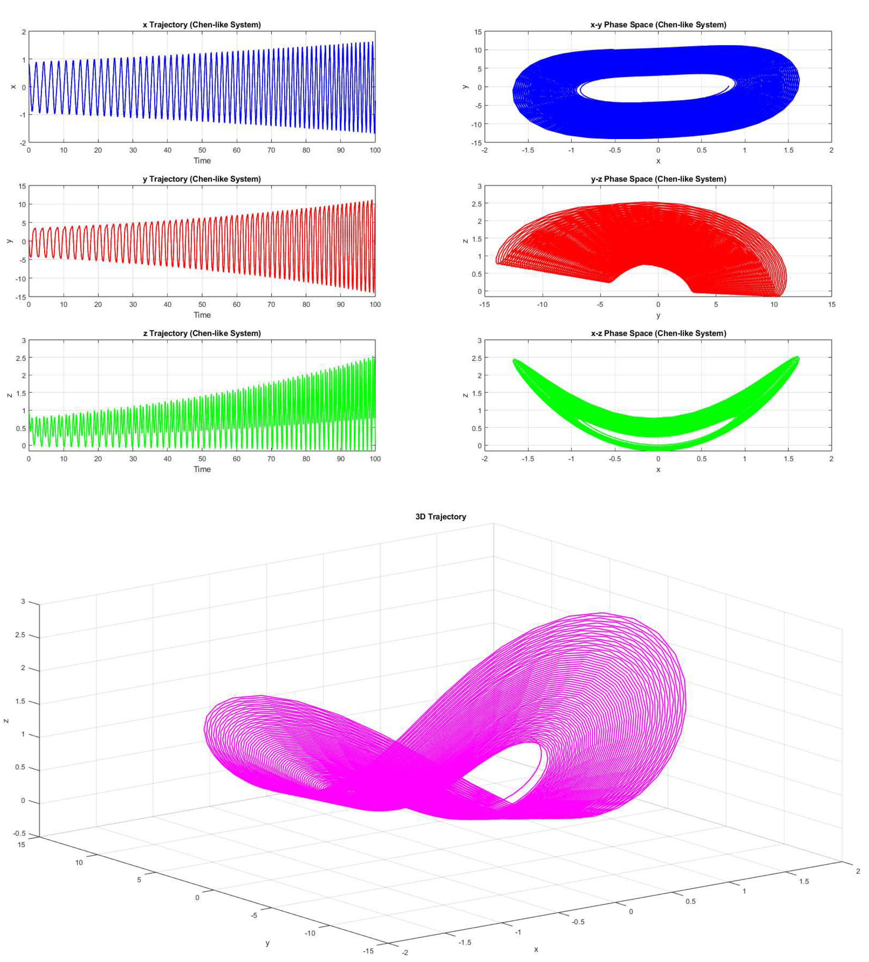
Figure 5.
Convergent trajectory in 3-dimension and 2-dimensional phase portraits
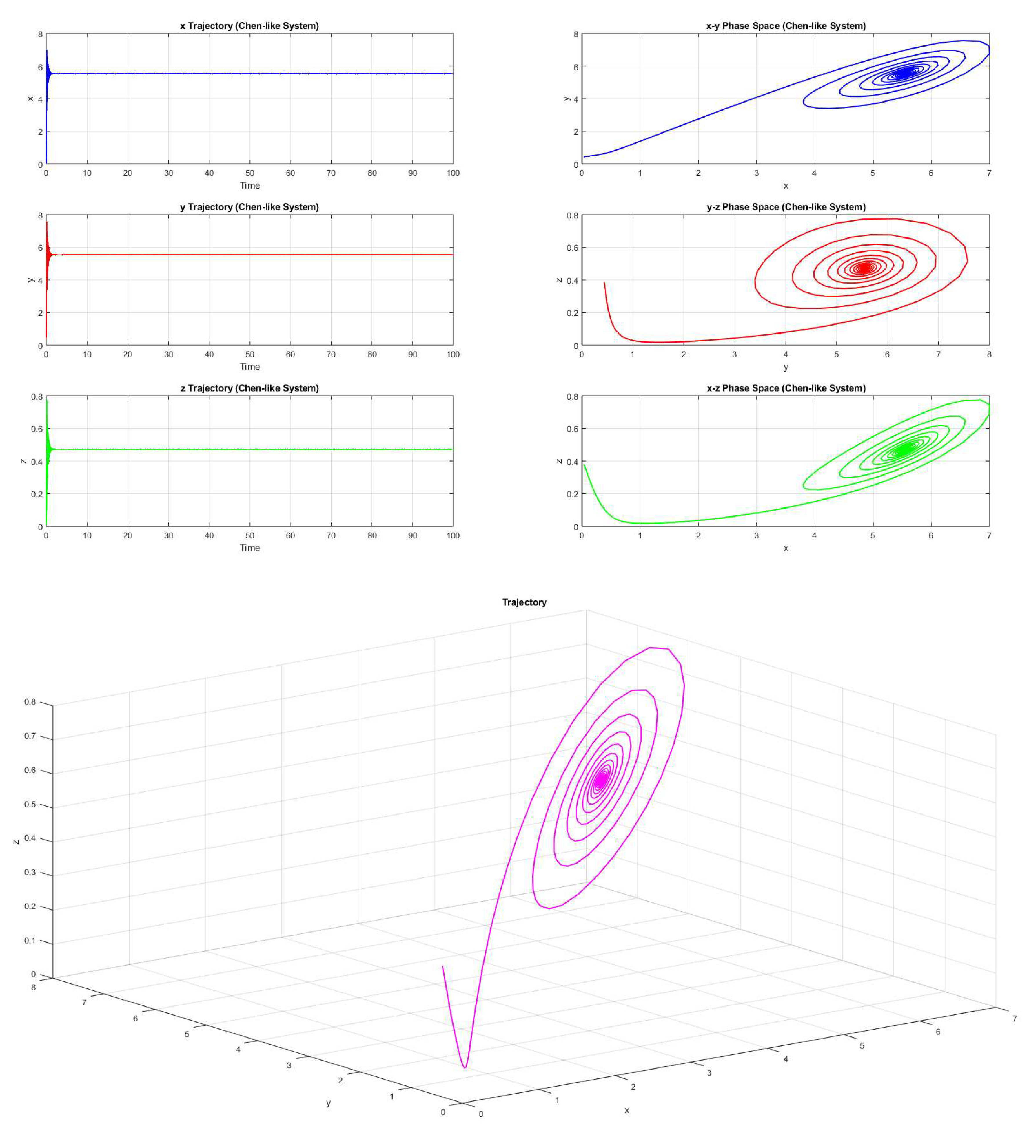
Figure 6.
Chaotic trajectory in 3 dimension and two dimensional phase portraits
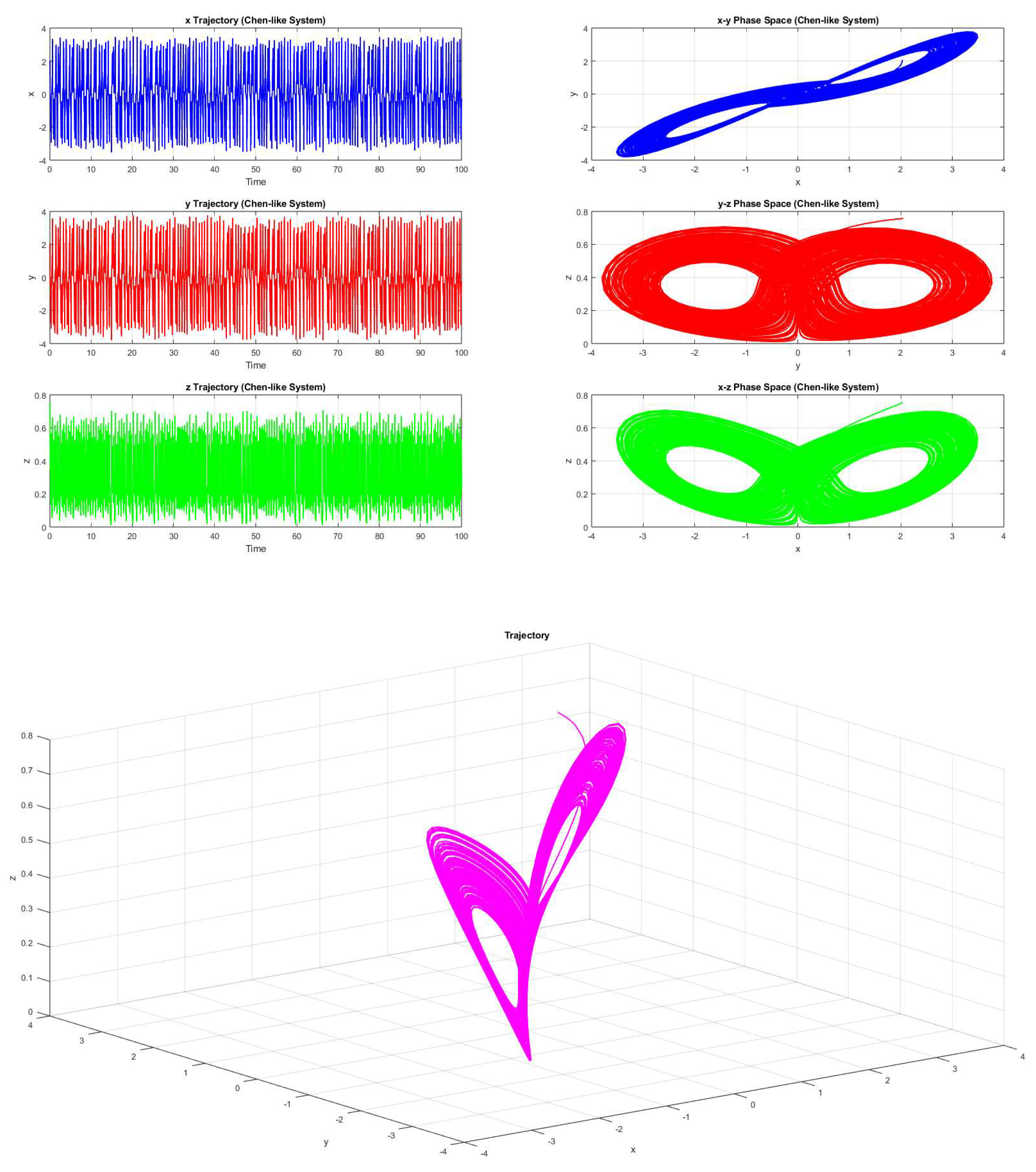
Figure 7.
Periodic trajectories with periodicity 69 and corresponding two dimensional phase portraits
Figure 7.
Periodic trajectories with periodicity 69 and corresponding two dimensional phase portraits
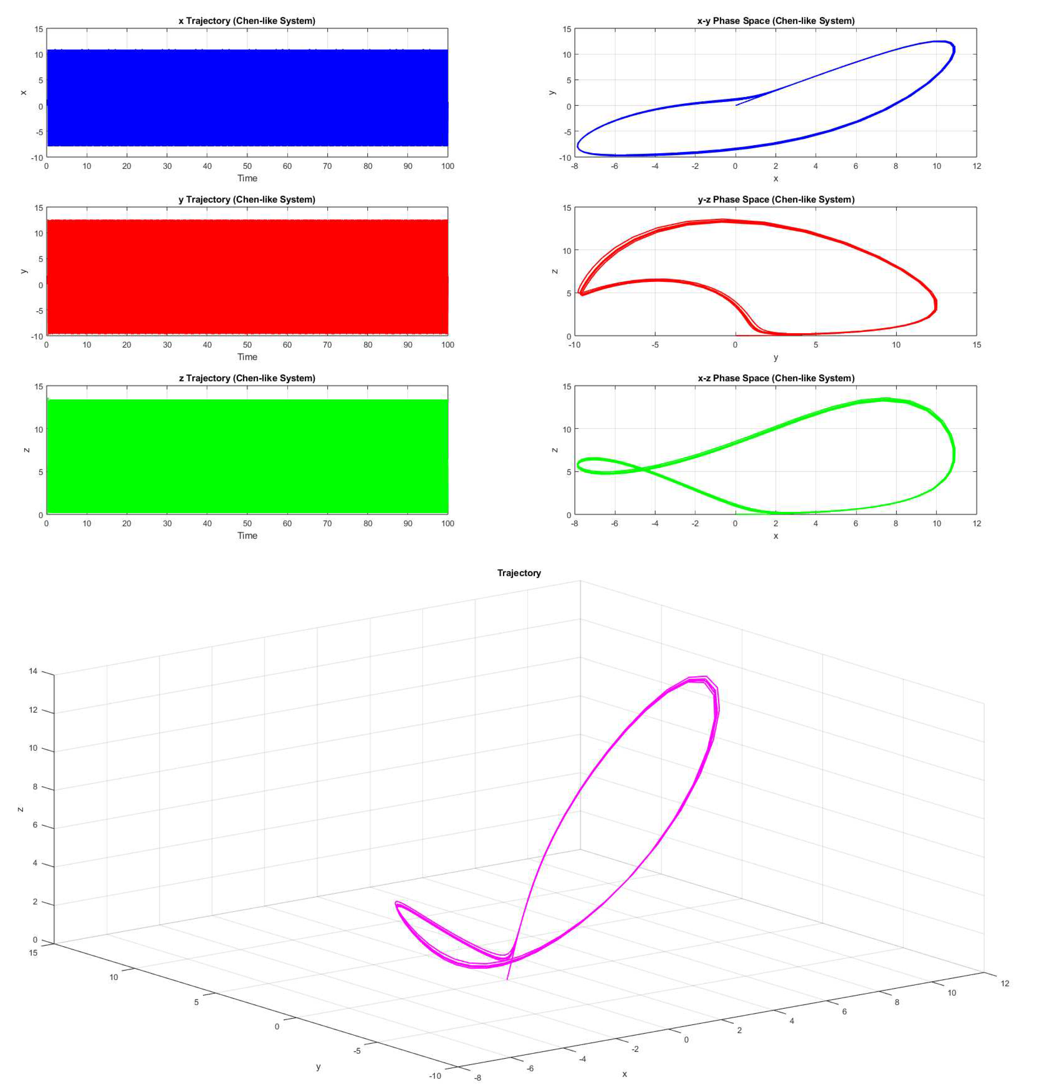
Figure 8.
Periodic trajectories with periodicity 425 and corresponding two dimensional phase portraits
Figure 8.
Periodic trajectories with periodicity 425 and corresponding two dimensional phase portraits
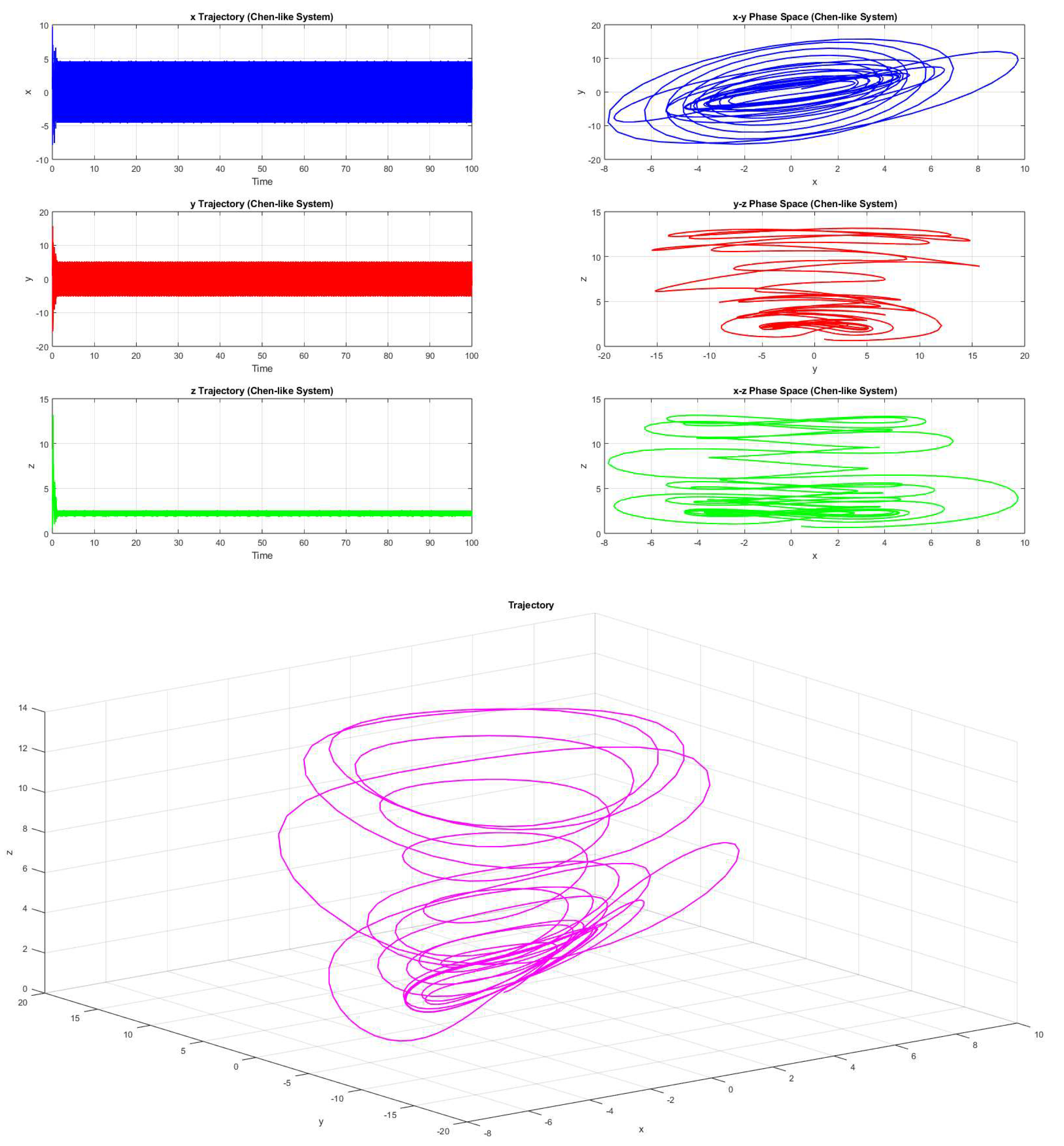
Figure 9.
Periodic trajectories with periodicity 689 and corresponding two dimensional phase portraits
Figure 9.
Periodic trajectories with periodicity 689 and corresponding two dimensional phase portraits
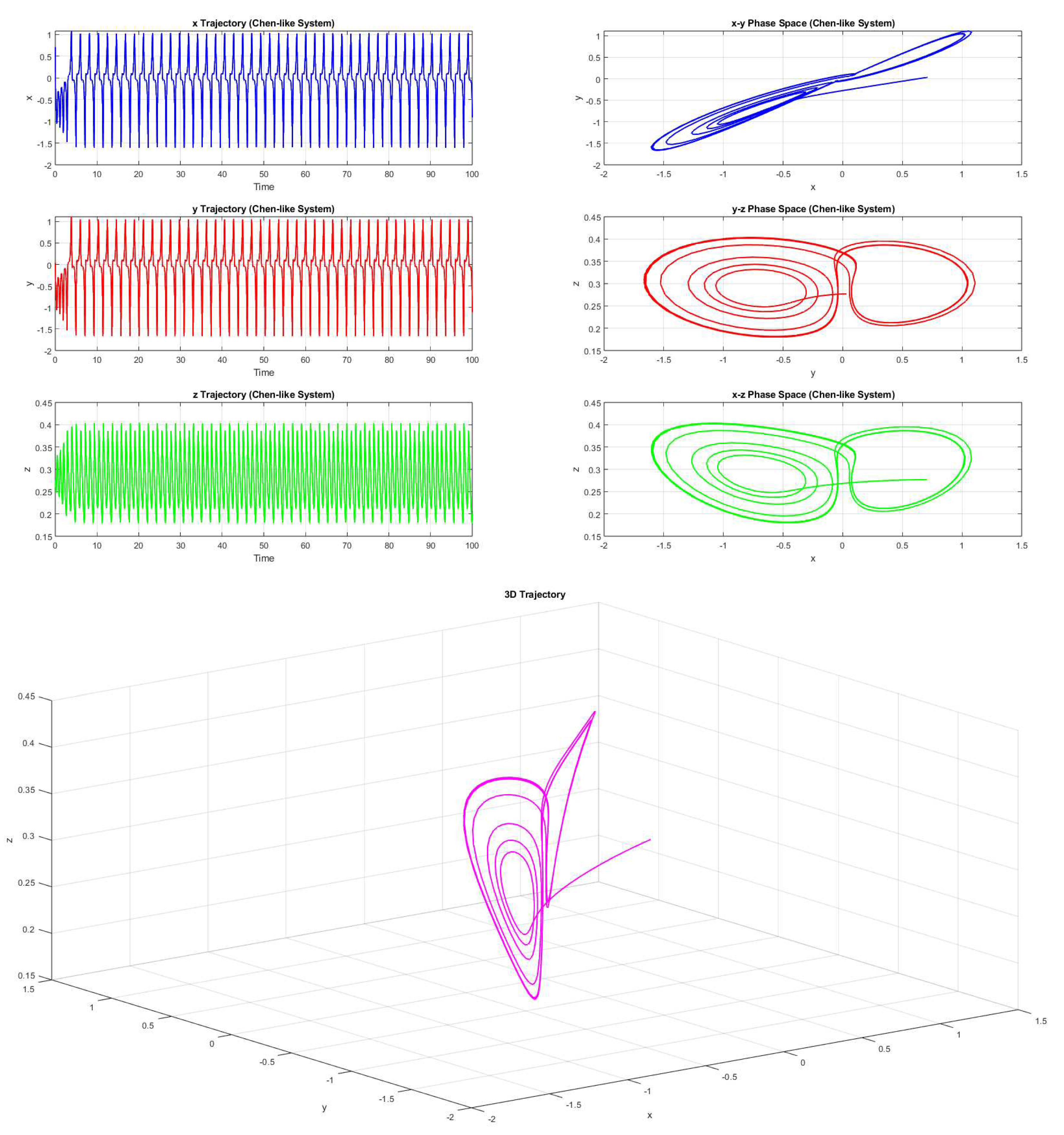
Figure 10.
Lyapunov exponent with associated parameters for 409 cases, where the system possesses chaotic trajectories.
Figure 10.
Lyapunov exponent with associated parameters for 409 cases, where the system possesses chaotic trajectories.
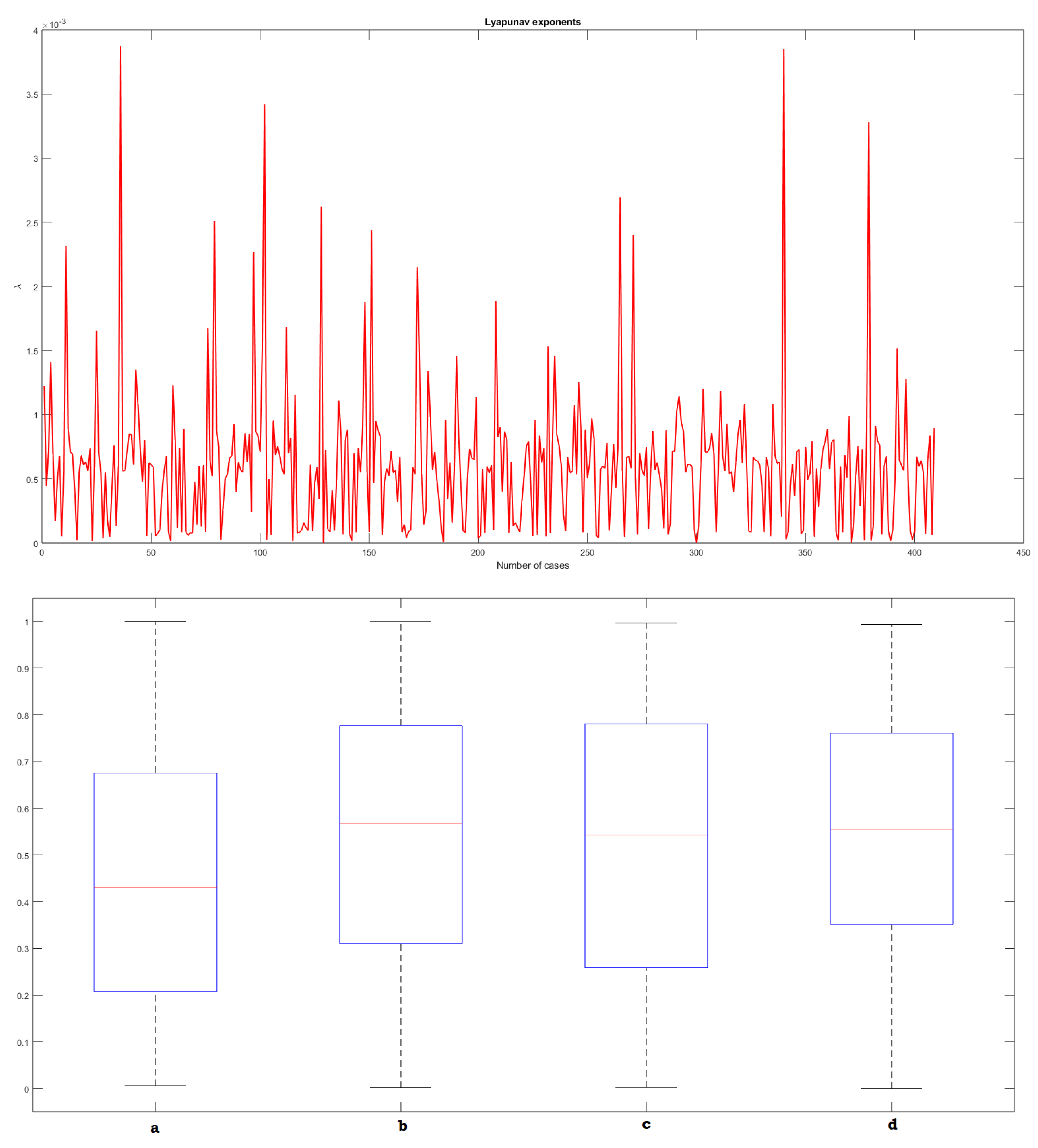
Figure 11.
Chaotic trajectories with Lyapunov exponent (=0.001220) and corresponding two dimensional phase portraits (Parameters: a=0.2575, b=0.8407, c=0.2543, and d=0.8143)
Figure 11.
Chaotic trajectories with Lyapunov exponent (=0.001220) and corresponding two dimensional phase portraits (Parameters: a=0.2575, b=0.8407, c=0.2543, and d=0.8143)
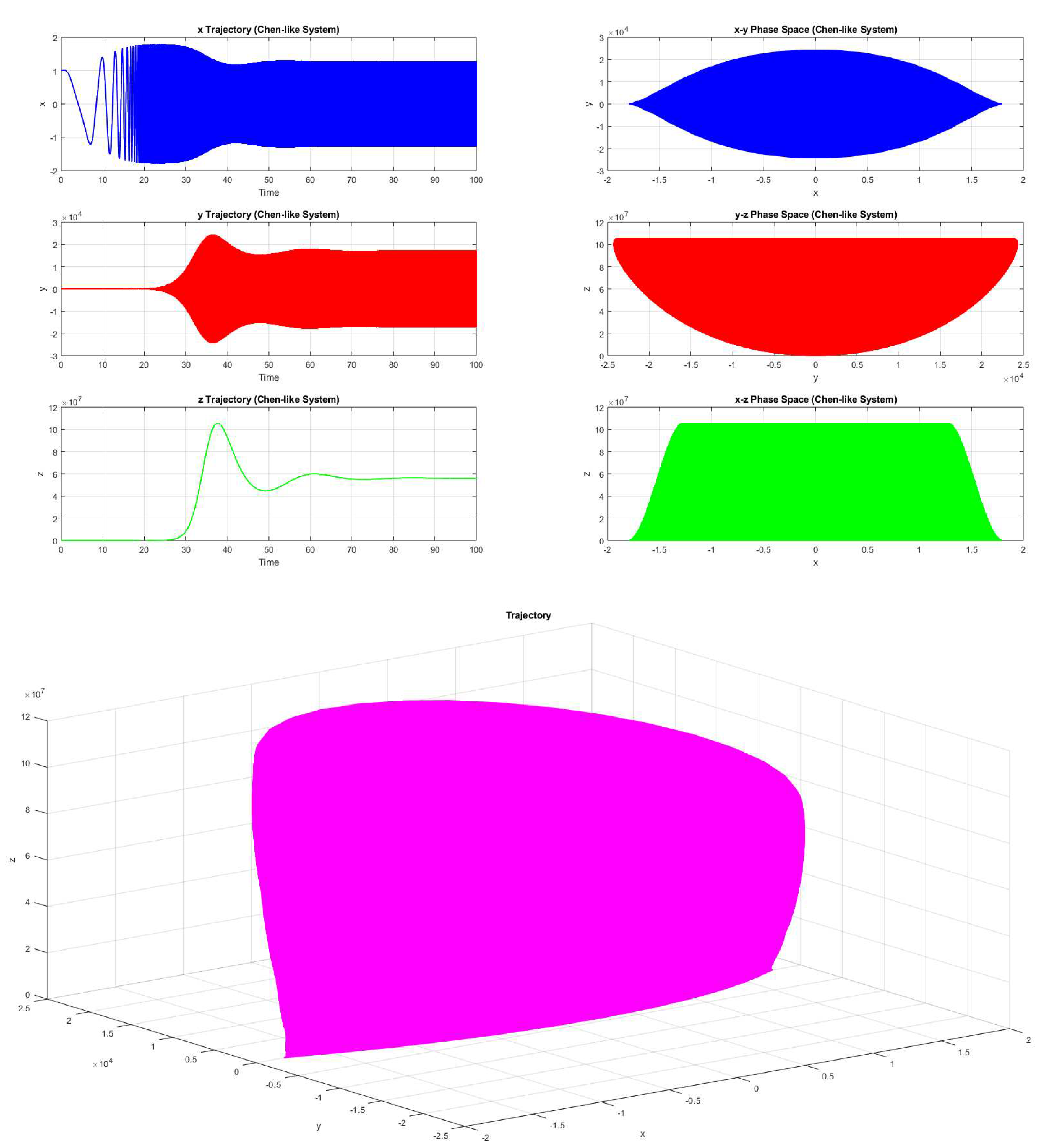
Figure 12.
Chaotic trajectories with Lyapunov exponent (=0.000094) and corresponding two dimensional phase portraits (Parameters: a=388, b=244, c=218, and d=224)
Figure 12.
Chaotic trajectories with Lyapunov exponent (=0.000094) and corresponding two dimensional phase portraits (Parameters: a=388, b=244, c=218, and d=224)
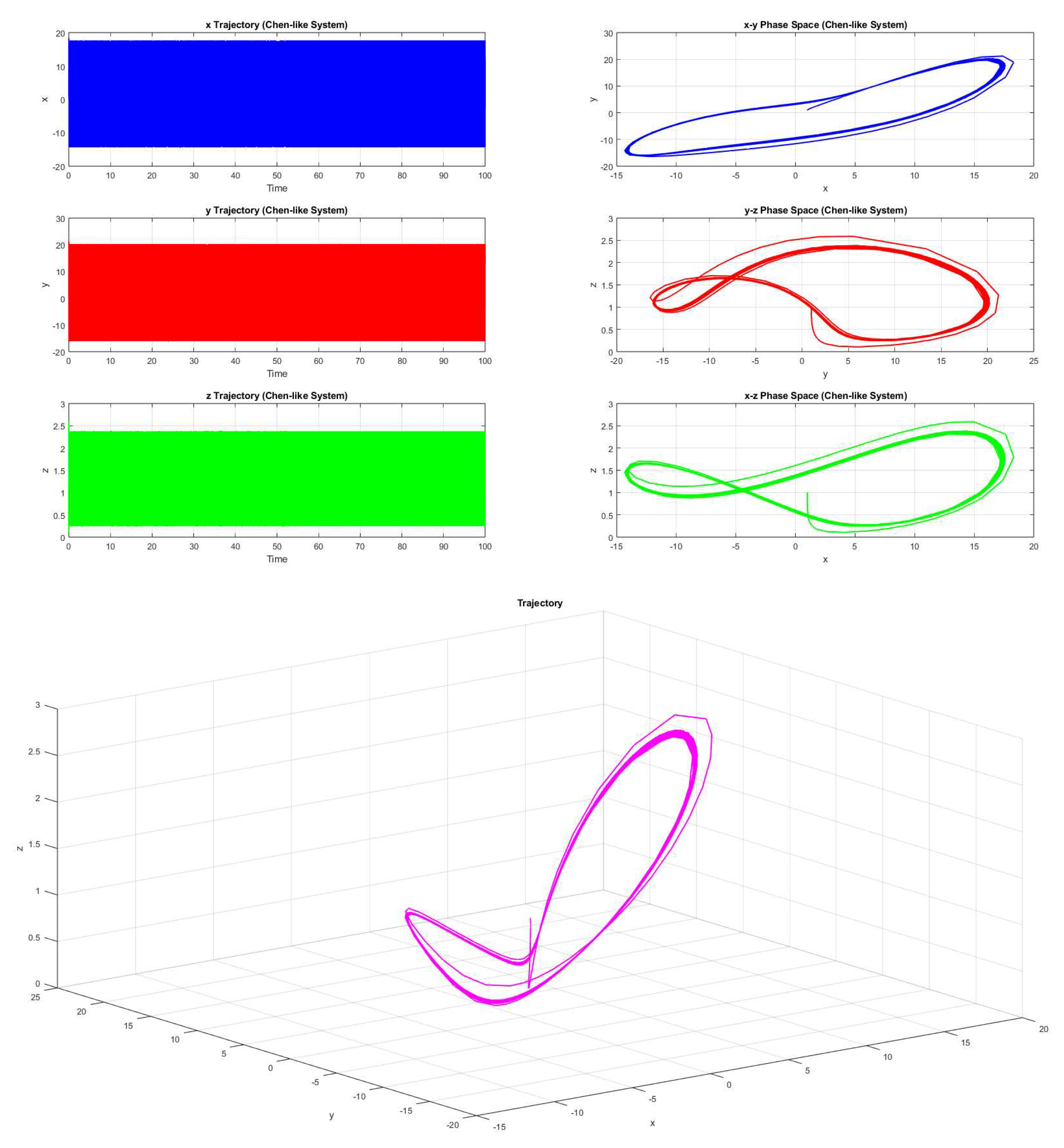
Figure 13.
Chaotic trajectories with Lyapunov exponent (=0.000088) and corresponding two dimensional phase portraits (Parameters: a=205, b=298, c=132, and d=302)
Figure 13.
Chaotic trajectories with Lyapunov exponent (=0.000088) and corresponding two dimensional phase portraits (Parameters: a=205, b=298, c=132, and d=302)
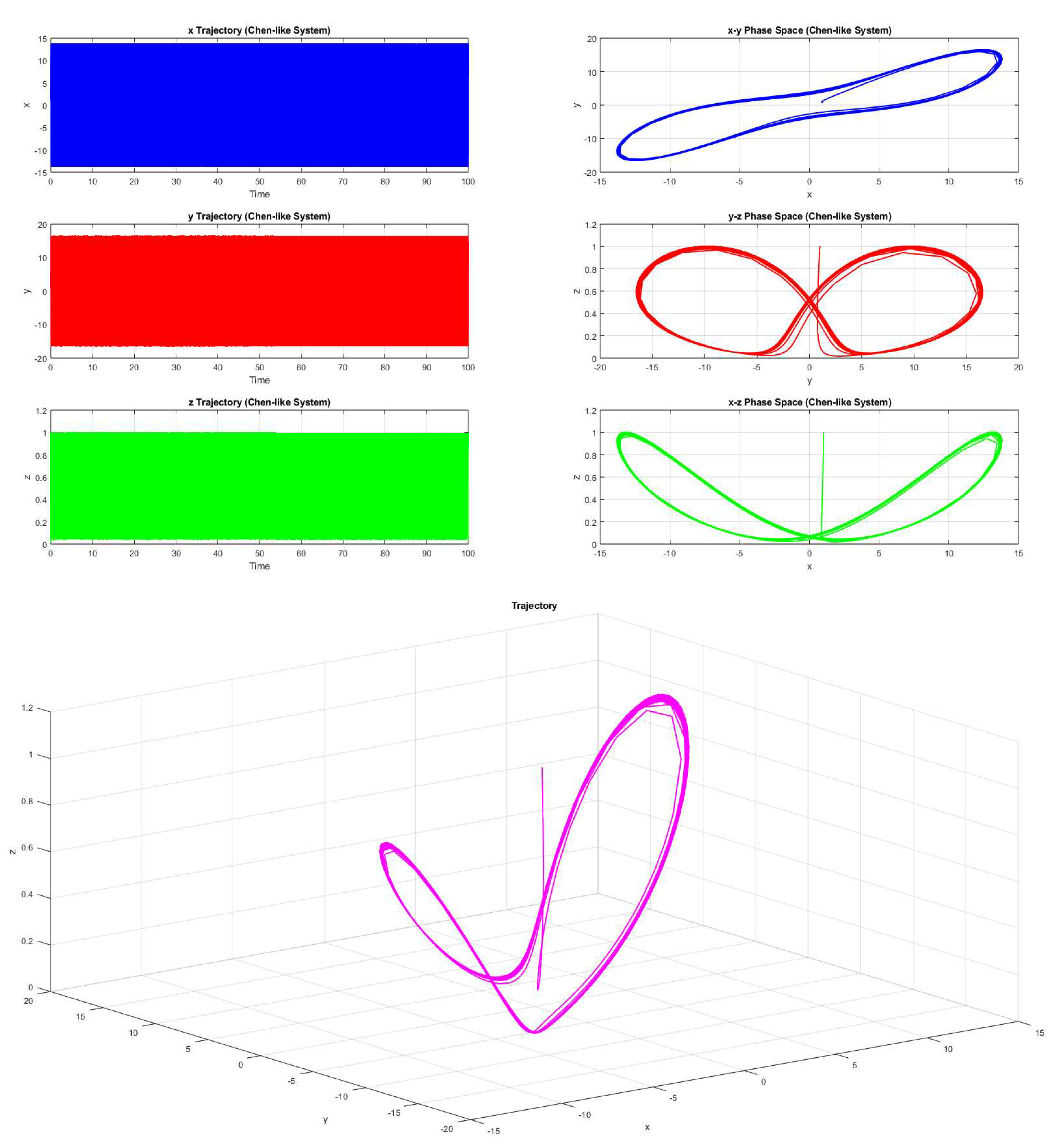
Figure 14.
Hopf Bifurcation diagram at where

Figure 15.
Hopf bifurcation for different set of parameters
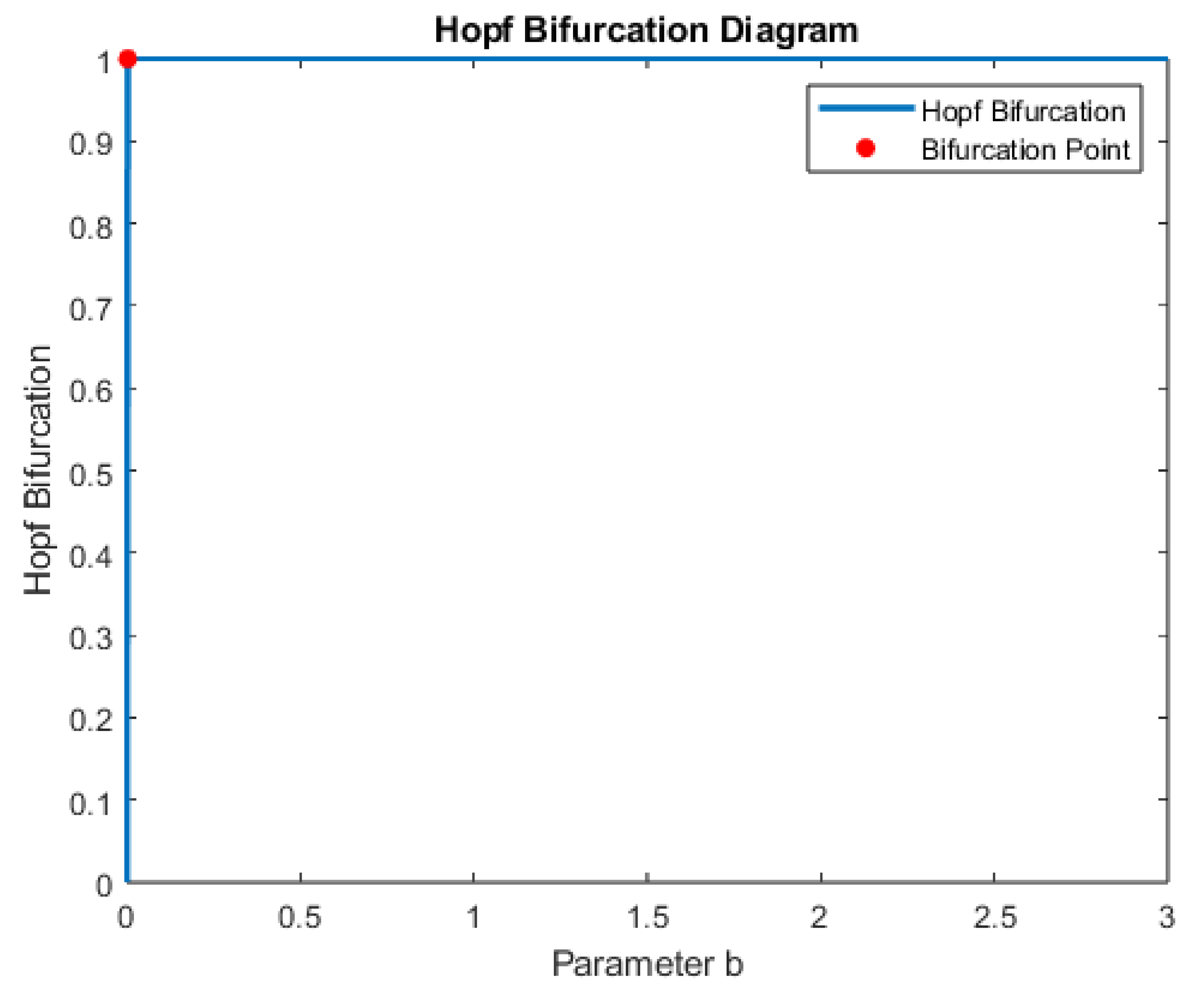

Table 1.
List of parameters and associated Lyapunov exponent for which chaotic were noticed in the model
Table 1.
List of parameters and associated Lyapunov exponent for which chaotic were noticed in the model
| a | b | c | d | Lambda | a | b | c | d | Lambda | a | b | c | d | Lambda | a | b | c | d | Lambda |
|---|---|---|---|---|---|---|---|---|---|---|---|---|---|---|---|---|---|---|---|
| 0.2575 | 0.8407 | 0.2543 | 0.8143 | 0.001220 | 0.7048 | 0.3810 | 0.0764 | 0.4108 | 0.000017 | 0.2732 | 0.3147 | 0.5817 | 0.6894 | 0.000626 | 0.7280 | 0.2020 | 0.7380 | 0.8672 | 0.000450 |
| 0.5285 | 0.1656 | 0.6020 | 0.2630 | 0.000442 | 0.0524 | 0.7343 | 0.4995 | 0.9433 | 0.001155 | 0.7750 | 0.7915 | 0.7095 | 0.9465 | 0.000738 | 0.2811 | 0.8722 | 0.8456 | 0.6480 | 0.000614 |
| 0.1450 | 0.8530 | 0.6221 | 0.3510 | 0.000713 | 0.6042 | 0.6411 | 0.1275 | 0.4962 | 0.000079 | 0.8880 | 0.0497 | 0.6702 | 0.9766 | 0.000053 | 0.6564 | 0.1693 | 0.6212 | 0.4246 | 0.000367 |
| 0.0154 | 0.0430 | 0.1690 | 0.6491 | 0.001406 | 0.6316 | 0.8335 | 0.2702 | 0.4008 | 0.000084 | 0.3218 | 0.9483 | 0.2073 | 0.4893 | 0.001529 | 0.1170 | 0.1304 | 0.7418 | 0.1383 | 0.000710 |
| 0.5502 | 0.6225 | 0.5870 | 0.2077 | 0.000694 | 0.6794 | 0.9768 | 0.1255 | 0.7522 | 0.000100 | 0.8777 | 0.8739 | 0.4896 | 0.6063 | 0.000080 | 0.4802 | 0.4346 | 0.5121 | 0.5245 | 0.000728 |
| 0.2625 | 0.8010 | 0.0292 | 0.9289 | 0.000169 | 0.9200 | 0.3001 | 0.0734 | 0.7674 | 0.000158 | 0.2179 | 0.7530 | 0.5198 | 0.7601 | 0.000793 | 0.7189 | 0.8807 | 0.0107 | 0.5715 | 0.000073 |
| 0.6596 | 0.5186 | 0.9730 | 0.6490 | 0.000490 | 0.9189 | 0.7336 | 0.3011 | 0.4956 | 0.000117 | 0.0338 | 0.8595 | 0.5286 | 0.9755 | 0.001459 | 0.7877 | 0.3098 | 0.1185 | 0.4854 | 0.000097 |
| 0.2691 | 0.4228 | 0.5479 | 0.9427 | 0.000677 | 0.9926 | 0.9322 | 0.0922 | 0.9535 | 0.000100 | 0.0641 | 0.4435 | 0.5430 | 0.5402 | 0.000844 | 0.3261 | 0.8255 | 0.5502 | 0.6448 | 0.000749 |
| 0.5830 | 0.2518 | 0.2904 | 0.6171 | 0.000053 | 0.4210 | 0.6401 | 0.7876 | 0.2700 | 0.000611 | 0.9678 | 0.6341 | 0.7773 | 0.8985 | 0.000758 | 0.3738 | 0.2585 | 0.2606 | 0.4725 | 0.000494 |
| 0.8200 | 0.7184 | 0.9686 | 0.5313 | 0.000557 | 0.8167 | 0.8301 | 0.4890 | 0.7607 | 0.000091 | 0.6803 | 0.8585 | 0.8718 | 0.8971 | 0.000601 | 0.6115 | 0.6153 | 0.8772 | 0.7669 | 0.000544 |
| 0.0067 | 0.6022 | 0.3868 | 0.9160 | 0.002314 | 0.3130 | 0.0764 | 0.7914 | 0.3654 | 0.000476 | 0.5240 | 0.0459 | 0.1013 | 0.4689 | 0.000222 | 0.3532 | 0.7589 | 0.5056 | 0.7658 | 0.000795 |
| 0.2089 | 0.7093 | 0.2362 | 0.1194 | 0.000887 | 0.1827 | 0.1012 | 0.2016 | 0.1347 | 0.000591 | 0.8595 | 0.7132 | 0.5750 | 0.7411 | 0.000095 | 0.9147 | 0.9990 | 0.1705 | 0.1726 | 0.000049 |
| 0.1097 | 0.0636 | 0.4046 | 0.4484 | 0.000710 | 0.5035 | 0.7688 | 0.3881 | 0.4533 | 0.000346 | 0.6022 | 0.6012 | 0.6439 | 0.9219 | 0.000667 | 0.2471 | 0.9018 | 0.9824 | 0.4841 | 0.000581 |
| 0.7487 | 0.8256 | 0.7900 | 0.3185 | 0.000692 | 0.0069 | 0.7666 | 0.0218 | 0.3931 | 0.002623 | 0.4282 | 0.1924 | 0.5675 | 0.6577 | 0.000548 | 0.7982 | 0.9952 | 0.2118 | 0.3290 | 0.000285 |
| 0.2467 | 0.6664 | 0.0835 | 0.6260 | 0.000406 | 0.4591 | 0.4329 | 0.2596 | 0.1337 | 0.000001 | 0.9743 | 0.5027 | 0.8914 | 0.7265 | 0.000557 | 0.2723 | 0.7312 | 0.9695 | 0.3756 | 0.000578 |
| 0.6952 | 0.4991 | 0.5358 | 0.4452 | 0.000019 | 0.2082 | 0.7573 | 0.5467 | 0.3574 | 0.000726 | 0.1108 | 0.8166 | 0.2493 | 0.5092 | 0.001074 | 0.1185 | 0.9190 | 0.6240 | 0.2576 | 0.000729 |
| 0.1339 | 0.0309 | 0.9391 | 0.3013 | 0.000553 | 0.7160 | 0.5529 | 0.1423 | 0.3804 | 0.000105 | 0.2271 | 0.1069 | 0.6628 | 0.9546 | 0.000537 | 0.1117 | 0.8468 | 0.6597 | 0.7797 | 0.000793 |
| 0.2089 | 0.9052 | 0.6754 | 0.4685 | 0.000681 | 0.6610 | 0.3947 | 0.2590 | 0.8479 | 0.000090 | 0.4890 | 0.8061 | 0.3778 | 0.5180 | 0.001251 | 0.0598 | 0.6160 | 0.5639 | 0.6683 | 0.000889 |
| 0.0899 | 0.0809 | 0.7772 | 0.9051 | 0.000610 | 0.8710 | 0.2118 | 0.8367 | 0.8593 | 0.000410 | 0.2397 | 0.9595 | 0.3055 | 0.1549 | 0.000896 | 0.4911 | 0.3418 | 0.9627 | 0.1249 | 0.000578 |
| 0.0729 | 0.0885 | 0.7984 | 0.9430 | 0.000632 | 0.5140 | 0.5484 | 0.2078 | 0.7846 | 0.000098 | 0.9380 | 0.6053 | 0.6389 | 0.7027 | 0.000081 | 0.0509 | 0.1350 | 0.5781 | 0.9044 | 0.000789 |
| 0.4845 | 0.1518 | 0.7819 | 0.1006 | 0.000563 | 0.6786 | 0.4651 | 0.9533 | 0.3547 | 0.000494 | 0.1808 | 0.9956 | 0.5204 | 0.8853 | 0.000885 | 0.2475 | 0.9359 | 0.5646 | 0.8796 | 0.000804 |
| 0.0594 | 0.3158 | 0.7727 | 0.6964 | 0.000739 | 0.3237 | 0.8011 | 0.2996 | 0.7756 | 0.001108 | 0.1879 | 0.0094 | 0.8383 | 0.4813 | 0.000508 | 0.6818 | 0.5632 | 0.1500 | 0.9862 | 0.000080 |
| 0.9879 | 0.1704 | 0.2578 | 0.3968 | 0.000018 | 0.1141 | 0.5408 | 0.4164 | 0.5171 | 0.000856 | 0.6218 | 0.4146 | 0.6476 | 0.4893 | 0.000619 | 0.6006 | 0.4361 | 0.1736 | 0.1949 | 0.000019 |
| 0.6537 | 0.9569 | 0.9357 | 0.4579 | 0.000592 | 0.4797 | 0.1987 | 0.2390 | 0.7802 | 0.000069 | 0.1788 | 0.8597 | 0.2320 | 0.1681 | 0.000970 | 0.4606 | 0.9209 | 0.8862 | 0.8795 | 0.000594 |
| 0.1807 | 0.2554 | 0.0205 | 0.9237 | 0.001652 | 0.3158 | 0.3113 | 0.3450 | 0.6663 | 0.000804 | 0.3937 | 0.9370 | 0.4369 | 0.1625 | 0.000816 | 0.8022 | 0.9645 | 0.1968 | 0.7781 | 0.000085 |
| 0.3833 | 0.6173 | 0.5755 | 0.5301 | 0.000702 | 0.1354 | 0.7655 | 0.3186 | 0.2524 | 0.000885 | 0.9406 | 0.5340 | 0.6712 | 0.6075 | 0.000061 | 0.3814 | 0.6192 | 0.6048 | 0.5356 | 0.000684 |
| 0.9456 | 0.6766 | 0.9883 | 0.7668 | 0.000549 | 0.8570 | 0.8998 | 0.3484 | 0.4863 | 0.000069 | 0.7173 | 0.9801 | 0.0537 | 0.6369 | 0.000042 | 0.5076 | 0.4991 | 0.9115 | 0.7303 | 0.000510 |
| 0.7043 | 0.7295 | 0.2243 | 0.2691 | 0.000036 | 0.6694 | 0.0372 | 0.0033 | 0.1425 | 0.000020 | 0.1299 | 0.2174 | 0.8934 | 0.6217 | 0.000573 | 0.0222 | 0.6580 | 0.4586 | 0.2000 | 0.000989 |
| 0.2815 | 0.2304 | 0.7111 | 0.6246 | 0.000551 | 0.3823 | 0.6929 | 0.6021 | 0.7753 | 0.000701 | 0.4606 | 0.7775 | 0.8168 | 0.6314 | 0.000601 | 0.9790 | 0.6826 | 0.7855 | 0.3488 | 0.000003 |
| 0.9227 | 0.8004 | 0.2859 | 0.5437 | 0.000178 | 0.5087 | 0.6033 | 0.1614 | 0.6355 | 0.000083 | 0.2535 | 0.6782 | 0.9145 | 0.6171 | 0.000582 | 0.6763 | 0.5017 | 0.1133 | 0.4613 | 0.000137 |
| 0.7284 | 0.5768 | 0.0259 | 0.4465 | 0.000048 | 0.1693 | 0.5934 | 0.6081 | 0.7724 | 0.000740 | 0.5198 | 0.6088 | 0.7272 | 0.0001 | 0.000777 | 0.3013 | 0.1542 | 0.7444 | 0.2829 | 0.000533 |
| 0.5989 | 0.1489 | 0.8997 | 0.4504 | 0.000410 | 0.4316 | 0.7179 | 0.9162 | 0.8900 | 0.000553 | 0.8823 | 0.5513 | 0.3215 | 0.8998 | 0.000097 | 0.0948 | 0.8065 | 0.6827 | 0.1732 | 0.000753 |
| 0.3249 | 0.2462 | 0.3427 | 0.3757 | 0.000759 | 0.2973 | 0.4044 | 0.3022 | 0.7573 | 0.000910 | 0.4824 | 0.0639 | 0.8029 | 0.3511 | 0.000412 | 0.5682 | 0.0123 | 0.5898 | 0.3602 | 0.000287 |
| 0.8266 | 0.3945 | 0.6135 | 0.8186 | 0.000135 | 0.0292 | 0.7798 | 0.5674 | 0.0761 | 0.001874 | 0.3136 | 0.7892 | 0.4983 | 0.4370 | 0.000768 | 0.4254 | 0.7827 | 0.5891 | 0.4721 | 0.000728 |
Table 2.
List of parameters and associated Lyapunov exponent for which chaotic were noticed in the model
Table 2.
List of parameters and associated Lyapunov exponent for which chaotic were noticed in the model
| a | b | c | d | Lambda | a | b | c | d | Lambda | a | b | c | d | Lambda | a | b | c | d | Lambda |
|---|---|---|---|---|---|---|---|---|---|---|---|---|---|---|---|---|---|---|---|
| 0.7343 | 0.4303 | 0.6938 | 0.9452 | 0.000597 | 0.1413 | 0.0793 | 0.8761 | 0.4204 | 0.000550 | 0.4327 | 0.0887 | 0.9351 | 0.3908 | 0.000427 | 0.9369 | 0.0359 | 0.1397 | 0.7254 | 0.000020 |
| 0.1432 | 0.5594 | 0.0046 | 0.7667 | 0.003872 | 0.8890 | 0.8598 | 0.5971 | 0.6548 | 0.000088 | 0.4991 | 0.2754 | 0.4196 | 0.5970 | 0.000739 | 0.1165 | 0.9812 | 0.5417 | 0.0865 | 0.000865 |
| 0.3002 | 0.4014 | 0.8334 | 0.4036 | 0.000562 | 0.0984 | 0.1700 | 0.3712 | 0.0398 | 0.002435 | 0.0055 | 0.1629 | 0.2623 | 0.0389 | 0.002692 | 0.1576 | 0.7601 | 0.0919 | 0.9677 | 0.003279 |
| 0.2649 | 0.0684 | 0.4363 | 0.1739 | 0.000566 | 0.8257 | 0.4445 | 0.9821 | 0.5783 | 0.000469 | 0.1315 | 0.0621 | 0.7775 | 0.7422 | 0.000557 | 0.9589 | 0.5074 | 0.6662 | 0.4295 | 0.000020 |
| 0.3365 | 0.1877 | 0.3219 | 0.4039 | 0.000716 | 0.0334 | 0.8390 | 0.5073 | 0.1137 | 0.000953 | 0.6163 | 0.0069 | 0.0629 | 0.9200 | 0.000045 | 0.5811 | 0.9684 | 0.0414 | 0.1886 | 0.000124 |
| 0.1982 | 0.6723 | 0.4315 | 0.6944 | 0.000848 | 0.2449 | 0.3790 | 0.2703 | 0.2156 | 0.000882 | 0.4317 | 0.5428 | 0.6101 | 0.4362 | 0.000667 | 0.6249 | 0.9417 | 0.5668 | 0.6931 | 0.000911 |
| 0.1519 | 0.3971 | 0.3747 | 0.1311 | 0.000843 | 0.0367 | 0.5384 | 0.7372 | 0.1812 | 0.000832 | 0.4002 | 0.5539 | 0.5963 | 0.5063 | 0.000676 | 0.0364 | 0.1939 | 0.7495 | 0.3082 | 0.000797 |
| 0.2299 | 0.5761 | 0.8106 | 0.4038 | 0.000611 | 0.9695 | 0.4421 | 0.5910 | 0.1110 | 0.000062 | 0.3649 | 0.5923 | 0.9052 | 0.2645 | 0.000580 | 0.1847 | 0.5737 | 0.4831 | 0.4216 | 0.000760 |
| 0.0610 | 0.5846 | 0.2851 | 0.8277 | 0.001353 | 0.7145 | 0.4598 | 0.9193 | 0.9889 | 0.000480 | 0.1063 | 0.5020 | 0.0192 | 0.4426 | 0.002400 | 0.8300 | 0.5672 | 0.2600 | 0.7845 | 0.000069 |
| 0.4139 | 0.3091 | 0.2638 | 0.7588 | 0.001083 | 0.8246 | 0.5375 | 0.8175 | 0.4604 | 0.000581 | 0.4569 | 0.2381 | 0.7712 | 0.2734 | 0.000508 | 0.9071 | 0.7020 | 0.8956 | 0.9480 | 0.000596 |
| 0.3963 | 0.7051 | 0.5586 | 0.7566 | 0.000735 | 0.3896 | 0.4901 | 0.8869 | 0.9050 | 0.000526 | 0.6639 | 0.7274 | 0.2230 | 0.5555 | 0.000066 | 0.3356 | 0.3110 | 0.4202 | 0.0877 | 0.000675 |
| 0.6153 | 0.3766 | 0.8772 | 0.7849 | 0.000479 | 0.7816 | 0.9877 | 0.7883 | 0.8529 | 0.000714 | 0.0800 | 0.7353 | 0.8227 | 0.3434 | 0.000700 | 0.9712 | 0.6034 | 0.6676 | 0.8633 | 0.000095 |
| 0.0496 | 0.0911 | 0.5940 | 0.2411 | 0.000800 | 0.4249 | 0.5216 | 0.8403 | 0.6250 | 0.000550 | 0.2798 | 0.7801 | 0.9628 | 0.6882 | 0.000572 | 0.9500 | 0.8285 | 0.6291 | 0.2956 | 0.000018 |
| 0.5481 | 0.3690 | 0.2083 | 0.4409 | 0.000059 | 0.3657 | 0.3449 | 0.6927 | 0.7166 | 0.000566 | 0.6764 | 0.7061 | 0.9577 | 0.9399 | 0.000526 | 0.7505 | 0.3189 | 0.1074 | 0.8061 | 0.000101 |
| 0.6181 | 0.9322 | 0.8351 | 0.8954 | 0.000624 | 0.3938 | 0.3918 | 0.2070 | 0.7245 | 0.000321 | 0.6356 | 0.8062 | 0.6679 | 0.2866 | 0.000744 | 0.3624 | 0.2311 | 0.8602 | 0.6344 | 0.000484 |
| 0.3253 | 0.8318 | 0.8103 | 0.5570 | 0.000613 | 0.4150 | 0.6873 | 0.6577 | 0.6800 | 0.000666 | 0.9315 | 0.9764 | 0.3312 | 0.6237 | 0.000110 | 0.0054 | 0.3653 | 0.5920 | 0.9248 | 0.001517 |
| 0.5464 | 0.3467 | 0.6228 | 0.7966 | 0.000587 | 0.9387 | 0.6181 | 0.2507 | 0.1025 | 0.000085 | 0.3075 | 0.4112 | 0.8163 | 0.3683 | 0.000572 | 0.6527 | 0.6747 | 0.7498 | 0.3059 | 0.000646 |
| 0.4380 | 0.9403 | 0.0058 | 0.6103 | 0.000057 | 0.5199 | 0.7663 | 0.3362 | 0.6260 | 0.000146 | 0.0248 | 0.9178 | 0.6860 | 0.2343 | 0.000874 | 0.6584 | 0.8083 | 0.8564 | 0.7109 | 0.000605 |
| 0.7425 | 0.7579 | 0.3891 | 0.4293 | 0.000074 | 0.7799 | 0.7083 | 0.5909 | 0.3770 | 0.000042 | 0.5430 | 0.3571 | 0.6616 | 0.6787 | 0.000573 | 0.7197 | 0.7773 | 0.6450 | 0.3381 | 0.000565 |
| 0.9737 | 0.9723 | 0.6437 | 0.8601 | 0.000104 | 0.9352 | 0.9698 | 0.3753 | 0.9849 | 0.000089 | 0.1079 | 0.4457 | 0.9388 | 0.6338 | 0.000627 | 0.2998 | 0.6323 | 0.2358 | 0.4893 | 0.001279 |
| 0.5197 | 0.0590 | 0.8900 | 0.3302 | 0.000399 | 0.5805 | 0.6261 | 0.1111 | 0.2137 | 0.000100 | 0.2054 | 0.2597 | 0.9426 | 0.6416 | 0.000527 | 0.4746 | 0.2317 | 0.7810 | 0.6824 | 0.000478 |
| 0.4509 | 0.5511 | 0.8054 | 0.7009 | 0.000564 | 0.6283 | 0.3648 | 0.6366 | 0.8913 | 0.000590 | 0.6273 | 0.2059 | 0.9802 | 0.4378 | 0.000416 | 0.6635 | 0.6355 | 0.3402 | 0.7448 | 0.000093 |
| 0.5811 | 0.6372 | 0.6513 | 0.8646 | 0.000674 | 0.4924 | 0.7294 | 0.9550 | 0.7624 | 0.000539 | 0.2459 | 0.9477 | 0.0324 | 0.9062 | 0.000114 | 0.4792 | 0.4382 | 0.2552 | 0.1411 | 0.000030 |
| 0.8296 | 0.8222 | 0.5707 | 0.5718 | 0.000084 | 0.1889 | 0.4339 | 0.0456 | 0.6555 | 0.002148 | 0.2142 | 0.9058 | 0.2778 | 0.0971 | 0.000876 | 0.6830 | 0.9247 | 0.2917 | 0.4760 | 0.000091 |
| 0.9730 | 0.3650 | 0.3092 | 0.1209 | 0.000014 | 0.0413 | 0.4238 | 0.0756 | 0.3138 | 0.001462 | 0.8031 | 0.8766 | 0.0875 | 0.6679 | 0.000066 | 0.5615 | 0.8522 | 0.7275 | 0.5387 | 0.000672 |
| 0.2379 | 0.2436 | 0.1048 | 0.8584 | 0.001229 | 0.9928 | 0.3901 | 0.8268 | 0.9541 | 0.000539 | 0.9952 | 0.4396 | 0.1514 | 0.7781 | 0.000150 | 0.2413 | 0.5041 | 0.8013 | 0.6635 | 0.000596 |
| 0.0686 | 0.2994 | 0.5916 | 0.2033 | 0.000800 | 0.5444 | 0.8461 | 0.0407 | 0.3294 | 0.000146 | 0.1912 | 0.3784 | 0.2563 | 0.0215 | 0.000720 | 0.3361 | 0.4643 | 0.3777 | 0.0640 | 0.000643 |
| 0.8169 | 0.1895 | 0.1237 | 0.8210 | 0.000118 | 0.7252 | 0.9120 | 0.0864 | 0.5200 | 0.000250 | 0.1148 | 0.8123 | 0.6668 | 0.3818 | 0.000714 | 0.5724 | 0.4917 | 0.8015 | 0.4411 | 0.000555 |
| 0.2470 | 0.3107 | 0.4089 | 0.7080 | 0.000739 | 0.0082 | 0.3984 | 0.4878 | 0.6181 | 0.001342 | 0.0933 | 0.9693 | 0.1900 | 0.1646 | 0.001033 | 0.9976 | 0.3841 | 0.5293 | 0.7842 | 0.000073 |
| 0.4334 | 0.7413 | 0.0705 | 0.8473 | 0.000084 | 0.0899 | 0.8103 | 0.3996 | 0.6553 | 0.000979 | 0.5752 | 0.9760 | 0.4416 | 0.7778 | 0.001142 | 0.4637 | 0.4008 | 0.9439 | 0.0956 | 0.000641 |
| 0.2988 | 0.7040 | 0.3816 | 0.5677 | 0.000891 | 0.4239 | 0.7993 | 0.9323 | 0.4697 | 0.000569 | 0.0343 | 0.5162 | 0.6533 | 0.7541 | 0.000943 | 0.0703 | 0.3794 | 0.5652 | 0.7566 | 0.000838 |
| 0.8776 | 0.4691 | 0.4374 | 0.7462 | 0.000080 | 0.1177 | 0.6573 | 0.7530 | 0.7021 | 0.000711 | 0.1665 | 0.7477 | 0.3346 | 0.3051 | 0.000874 | 0.4658 | 0.7984 | 0.2210 | 0.3824 | 0.000060 |
| 0.7896 | 0.7992 | 0.0496 | 0.2832 | 0.000063 | 0.8236 | 0.4272 | 0.9203 | 0.5280 | 0.000482 | 0.4630 | 0.1669 | 0.4664 | 0.4564 | 0.000550 | 0.0851 | 0.0490 | 0.0804 | 0.2133 | 0.000897 |
Table 3.
List of parameters and associated Lyapunov exponent for which chaotic were noticed in the model
Table 3.
List of parameters and associated Lyapunov exponent for which chaotic were noticed in the model
| a | b | c | d | Lambda | a | b | c | d | Lambda | a | b | c | d | Lambda |
|---|---|---|---|---|---|---|---|---|---|---|---|---|---|---|
| 0.9852 | 0.6088 | 0.2537 | 0.1326 | 0.000079 | 0.3433 | 0.0786 | 0.3022 | 0.3004 | 0.000327 | 0.3547 | 0.6377 | 0.7498 | 0.4924 | 0.000614 |
| 0.7603 | 0.5841 | 0.4030 | 0.5100 | 0.000077 | 0.9997 | 0.1292 | 0.2934 | 0.4769 | 0.000114 | 0.3478 | 0.0713 | 0.8551 | 0.0944 | 0.000611 |
| 0.9820 | 0.5136 | 0.9926 | 0.4558 | 0.000475 | 0.1358 | 0.8583 | 0.0186 | 0.7283 | 0.000011 | 0.1763 | 0.6189 | 0.9703 | 0.6692 | 0.000594 |
| 0.4939 | 0.8627 | 0.2429 | 0.8343 | 0.000143 | 0.2460 | 0.7278 | 0.2882 | 0.2373 | 0.000961 | 0.3644 | 0.8208 | 0.1228 | 0.6494 | 0.000090 |
| 0.1629 | 0.5659 | 0.9316 | 0.7831 | 0.000603 | 0.8600 | 0.0089 | 0.9960 | 0.2752 | 0.000346 | 0.7416 | 0.2173 | 0.3973 | 0.2626 | 0.000002 |
| 0.8506 | 0.1445 | 0.3705 | 0.6224 | 0.000133 | 0.4063 | 0.4302 | 0.6593 | 0.2184 | 0.000626 | 0.7028 | 0.4707 | 0.4089 | 0.9886 | 0.000127 |
| 0.2886 | 0.2690 | 0.5942 | 0.4759 | 0.000604 | 0.7944 | 0.8885 | 0.1425 | 0.9397 | 0.000158 | 0.6875 | 0.7257 | 0.8465 | 0.5538 | 0.000604 |
| 0.3567 | 0.7529 | 0.1100 | 0.5970 | 0.000089 | 0.4310 | 0.7649 | 0.9965 | 0.2650 | 0.000568 | 0.0995 | 0.0909 | 0.0342 | 0.3242 | 0.001201 |
| 0.2698 | 0.9897 | 0.1837 | 0.8617 | 0.001676 | 0.0478 | 0.6983 | 0.2571 | 0.6909 | 0.001453 | 0.7368 | 0.8340 | 0.8363 | 0.0331 | 0.000709 |
| 0.3044 | 0.9677 | 0.8960 | 0.1900 | 0.000635 | 0.0539 | 0.7870 | 0.6301 | 0.5088 | 0.000830 | 0.4332 | 0.3384 | 0.4547 | 0.7700 | 0.000707 |
| 0.2472 | 0.0542 | 0.6090 | 0.7772 | 0.000518 | 0.9827 | 0.6822 | 0.8709 | 0.4962 | 0.000447 | 0.5214 | 0.9418 | 0.6375 | 0.7186 | 0.000740 |
| 0.0346 | 0.4511 | 0.0138 | 0.4737 | 0.002510 | 0.9557 | 0.3079 | 0.3423 | 0.3870 | 0.000100 | 0.2006 | 0.2876 | 0.2926 | 0.4298 | 0.000856 |
| 0.1203 | 0.6255 | 0.3466 | 0.3346 | 0.000878 | 0.3951 | 0.4373 | 0.0849 | 0.5814 | 0.000079 | 0.2993 | 0.7754 | 0.6424 | 0.1795 | 0.000698 |
| 0.3298 | 0.2042 | 0.7672 | 0.0700 | 0.000747 | 0.5073 | 0.4858 | 0.8617 | 0.9655 | 0.000513 | 0.6076 | 0.7765 | 0.0635 | 0.5912 | 0.000083 |
| 0.9685 | 0.0988 | 0.5470 | 0.4030 | 0.000026 | 0.2315 | 0.3811 | 0.4532 | 0.5006 | 0.000736 | 0.2458 | 0.6336 | 0.9601 | 0.7264 | 0.000566 |
| 0.8325 | 0.9954 | 0.6498 | 0.7040 | 0.000268 | 0.4472 | 0.6410 | 0.6489 | 0.6784 | 0.000662 | 0.0117 | 0.7284 | 0.4153 | 0.1186 | 0.001182 |
| 0.3472 | 0.2537 | 0.9525 | 0.2982 | 0.000504 | 0.9804 | 0.7128 | 0.8257 | 0.6832 | 0.000651 | 0.2890 | 0.1431 | 0.3081 | 0.3474 | 0.000678 |
| 0.5088 | 0.5305 | 0.8597 | 0.6777 | 0.000536 | 0.0450 | 0.8420 | 0.1647 | 0.1151 | 0.001136 | 0.6256 | 0.9258 | 0.9832 | 0.7232 | 0.000561 |
| 0.2343 | 0.4647 | 0.6194 | 0.6153 | 0.000664 | 0.3751 | 0.1463 | 0.3168 | 0.2812 | 0.000039 | 0.4070 | 0.2738 | 0.2314 | 0.7379 | 0.000929 |
| 0.5835 | 0.0833 | 0.6602 | 0.0523 | 0.000679 | 0.9805 | 0.3267 | 0.2196 | 0.5182 | 0.000058 | 0.5232 | 0.1247 | 0.4527 | 0.9926 | 0.000540 |
| 0.6065 | 0.7146 | 0.4015 | 0.8587 | 0.000925 | 0.0064 | 0.9199 | 0.0180 | 0.0294 | 0.000573 | 0.3319 | 0.3223 | 0.7654 | 0.3842 | 0.000556 |
| 0.5311 | 0.0015 | 0.8838 | 0.4044 | 0.000397 | 0.9911 | 0.9511 | 0.6382 | 0.5041 | 0.000078 | 0.6393 | 0.1252 | 0.8653 | 0.4878 | 0.000395 |
| 0.6505 | 0.8914 | 0.8611 | 0.2099 | 0.000628 | 0.1013 | 0.0719 | 0.9045 | 0.3118 | 0.000594 | 0.5931 | 0.7313 | 0.6531 | 0.0620 | 0.000623 |
| 0.6862 | 0.3767 | 0.5043 | 0.7635 | 0.000572 | 0.5703 | 0.8515 | 0.9846 | 0.7902 | 0.000548 | 0.2816 | 0.5434 | 0.4072 | 0.9203 | 0.000842 |
| 0.3146 | 0.3820 | 0.7915 | 0.8392 | 0.000550 | 0.5520 | 0.7423 | 0.8246 | 0.3934 | 0.000604 | 0.1329 | 0.5612 | 0.2076 | 0.1180 | 0.000963 |
| 0.1698 | 0.1787 | 0.2435 | 0.7518 | 0.000856 | 0.7118 | 0.2149 | 0.0154 | 0.2100 | 0.000107 | 0.3792 | 0.9956 | 0.8695 | 0.9479 | 0.000626 |
| 0.5167 | 0.1519 | 0.3807 | 0.8210 | 0.000631 | 0.0778 | 0.2414 | 0.0258 | 0.8465 | 0.001885 | 0.2946 | 0.6510 | 0.2986 | 0.9447 | 0.001081 |
| 0.0708 | 0.9248 | 0.6421 | 0.1045 | 0.000847 | 0.2448 | 0.7272 | 0.4008 | 0.3106 | 0.000826 | 0.3535 | 0.6411 | 0.7716 | 0.6771 | 0.000602 |
| 0.6539 | 0.6577 | 0.1610 | 0.4324 | 0.000244 | 0.3131 | 0.6074 | 0.3787 | 0.9255 | 0.000902 | 0.4389 | 0.5872 | 0.3070 | 0.4355 | 0.000089 |
| 0.1261 | 0.3001 | 0.0021 | 0.9511 | 0.002264 | 0.7783 | 0.4073 | 0.8270 | 0.1480 | 0.000399 | 0.3193 | 0.2194 | 0.0280 | 0.6802 | 0.000086 |
| 0.1664 | 0.1496 | 0.2027 | 0.9550 | 0.000867 | 0.6216 | 0.9116 | 0.6061 | 0.4853 | 0.000867 | 0.3071 | 0.6262 | 0.6340 | 0.3012 | 0.000668 |
| 0.1695 | 0.8837 | 0.3879 | 0.3826 | 0.000838 | 0.2181 | 0.3177 | 0.3440 | 0.8001 | 0.000807 | 0.8987 | 0.7888 | 0.9088 | 0.4214 | 0.000644 |
| 0.5223 | 0.3974 | 0.4791 | 0.9939 | 0.000712 | 0.4402 | 0.6050 | 0.1270 | 0.5990 | 0.000077 | 0.1888 | 0.4065 | 0.6940 | 0.8295 | 0.000641 |
| 0.0679 | 0.2079 | 0.0396 | 0.4694 | 0.001517 | 0.1848 | 0.6454 | 0.8566 | 0.8534 | 0.000631 | 0.4091 | 0.6937 | 0.7808 | 0.6364 | 0.000606 |
| 0.1883 | 0.7592 | 0.0317 | 0.6423 | 0.003418 | 0.9706 | 0.5681 | 0.2740 | 0.1291 | 0.000133 | 0.6166 | 0.2398 | 0.7911 | 0.7056 | 0.000461 |
| 0.6617 | 0.6028 | 0.4738 | 0.3563 | 0.000030 | 0.9551 | 0.0630 | 0.1832 | 0.6242 | 0.000159 | 0.7175 | 0.6209 | 0.3761 | 0.6307 | 0.000085 |
| 0.1844 | 0.0457 | 0.8850 | 0.8398 | 0.000498 | 0.5963 | 0.7235 | 0.4081 | 0.5976 | 0.000118 | 0.1032 | 0.8175 | 0.9801 | 0.7517 | 0.000667 |
| 0.5135 | 0.8144 | 0.0972 | 0.4637 | 0.000064 | 0.6701 | 0.9817 | 0.2561 | 0.6192 | 0.000086 | 0.3786 | 0.7838 | 0.9141 | 0.3611 | 0.000582 |
| 0.1336 | 0.6385 | 0.3849 | 0.7657 | 0.000956 | 0.8205 | 0.0398 | 0.9662 | 0.8880 | 0.000329 | 0.2949 | 0.2728 | 0.0809 | 0.1863 | 0.000055 |
| 0.1253 | 0.3645 | 0.6762 | 0.3758 | 0.000684 | 0.5353 | 0.3116 | 0.7086 | 0.5871 | 0.000527 | 0.0735 | 0.9880 | 0.4279 | 0.7590 | 0.001082 |
| 0.1514 | 0.1496 | 0.3508 | 0.3360 | 0.000753 | 0.4198 | 0.3967 | 0.4129 | 0.9740 | 0.000757 | 0.1200 | 0.4120 | 0.7981 | 0.2527 | 0.000678 |
| 0.0785 | 0.2376 | 0.8176 | 0.4058 | 0.000674 | 0.6063 | 0.7643 | 0.6006 | 0.7226 | 0.000788 | 0.0911 | 0.3132 | 0.9583 | 0.6385 | 0.000620 |
| 0.2631 | 0.1027 | 0.4837 | 0.4189 | 0.000577 | 0.5031 | 0.3827 | 0.9772 | 0.9361 | 0.000460 | 0.8447 | 0.8828 | 0.9283 | 0.5626 | 0.000631 |
| 0.9043 | 0.6302 | 0.9830 | 0.5852 | 0.000536 | 0.6203 | 0.0898 | 0.1118 | 0.5756 | 0.000057 | 0.8976 | 0.2379 | 0.0671 | 0.3656 | 0.000206 |
| 0.0611 | 0.2195 | 0.0828 | 0.9504 | 0.001682 | 0.0898 | 0.6838 | 0.5469 | 0.9860 | 0.000960 | 0.0781 | 0.5259 | 0.0451 | 0.7966 | 0.003848 |
| 0.2038 | 0.9587 | 0.7118 | 0.1669 | 0.000699 | 0.4253 | 0.1058 | 0.0431 | 0.5561 | 0.000062 | 0.5610 | 0.2459 | 0.1345 | 0.2376 | 0.000030 |
| 0.0268 | 0.5004 | 0.8270 | 0.2590 | 0.000819 | 0.2468 | 0.3695 | 0.3411 | 0.4564 | 0.000837 | 0.8422 | 0.9715 | 0.1429 | 0.8569 | 0.000086 |
Disclaimer/Publisher’s Note: The statements, opinions and data contained in all publications are solely those of the individual author(s) and contributor(s) and not of MDPI and/or the editor(s). MDPI and/or the editor(s) disclaim responsibility for any injury to people or property resulting from any ideas, methods, instructions or products referred to in the content. |
© 2023 by the authors. Licensee MDPI, Basel, Switzerland. This article is an open access article distributed under the terms and conditions of the Creative Commons Attribution (CC BY) license (http://creativecommons.org/licenses/by/4.0/).
Copyright: This open access article is published under a Creative Commons CC BY 4.0 license, which permit the free download, distribution, and reuse, provided that the author and preprint are cited in any reuse.


