PM-Gati Shakti: A Case Study of Demand Forecasting

SujayKumar Reddy M; Gopakumar G

doi:10.20944/preprints202308.0535.v1

Submitted:

06 August 2023

Posted:

07 August 2023

You are already at the latest version

Abstract

PM-Gati-Shakti Initiative, integration of ministries, including railways, ports, waterways, logistic infrastructure, mass transport, airports, and roads. Aimed at enhancing connectivity and bolstering the competitiveness of Indian businesses, the initiative focuses on six pivotal pillars known as "Connectivity for Productivity": comprehensiveness, prioritization, optimization, synchronization, analytical, and dynamic. In this study, we explore the application of these pillars to address the problem of "Maximum Demand Forecasting in Delhi." Electricity forecasting plays a very significant role in the power grid as it is required to maintain a balance between supply and load demand at all times, to provide a quality electricity supply, for Financial planning, generation reserve, and many more. Forecasting helps not only in Production Planning but also in Scheduling like Import / Export which is very often in India and mostly required by the rural areas and North Eastern Regions of India. As Electrical Forecasting includes many factors which cannot be detected by the models out there, We use Classical Forecasting Techniques to extract the seasonal patterns from the daily data of Maximum Demand for the Union Territory Delhi. This research contributes to the power supply industry by helping to reduce the occurrence of disasters such as blackouts, power cuts, and increased tariffs imposed by regulatory commissions. The forecasting techniques can also help in reducing OD and UD of Power for different regions. We use the Data provided by a department from the Ministry of Power and use different forecast models including Seasonal forecasts for daily data.

Keywords:

Machine Learning

;

Time-Series Forecasting

;

Demand Forecasting

;

PM Gati-Shakti

;

Ministry of Power

;

Delhi

Subject:

Computer Science and Mathematics - Artificial Intelligence and Machine Learning

Introduction

The Indian Energy GRID is maintained by POWERGRID [18] which has the objectives of running the GRID efficiently and installing transmission lines etc... and the second one is the National Load Dispatch Center (NLDC) [14] which concentrates on Supervision over the Regional Load Dispatch Centres, Scheduling and dispatch of electricity over inter-regional links in accordance with grid standards specified by the Authority and grid code specified by Central Commission in coordination with Regional Load Dispatch Centres, Monitoring of operations and grid security of the National Grid, etc... This research mainly focusses on this NLDC which is a Division of Ministry of Power.

Figure 1 [15] describes the Yearly Installed Power Capacity in Delhi. The highest installed Capacity was 8,346.72 MW in Fiscal year 2016. which is responsible for sending the energy from Stations to sub-stations and to discuss and then to homes, industries, commercials, etc... As of 21-06-2023 The installed Capacity Sector-wise data [16] gives an overview of what type of Thermal Plants which are present in Delhi and also what types of Energy resources are present in Delhi. There are 11 Thermal Stations in Delhi with 4 400KV Substations and 42 200 KV Substations [17].

Delhi Yearly Power Statistics

To further Analyse Delhi’s Power, this paper uses the [15] RBI’s handbook contains yearly state-wise data to analyze the Delhi v/s Whole India’s data. Figure 2(a) gives Delhi v/s whole India’s Statewise Per-capita of Power raises to 1974.4 Kilo-Watt Hour in Delhi in 2018-2019 and in India 1115.3 Kilo-Watt Hours in 2021-2022. Figure 2(b) gives an Availability of Power at Delhi raises to 3308 net Crore Units in 2019-2020 and 137402 net crore units in 2021-2022 for All India, Figure 2(c) gives the Total Installed Capacity of RES Power raises to 245 Mega Watt at 2021 for Delhi and 94434 MegaWatt at 2021 for all India. Figure 2(d) depicts the Power Requirement for Delhi has the maximum reading at 3309 net crore units in 2019-2020 and for all of India 137981 net crore units in 2021-2022.

Relation to Demand Forecasting

The correlation between these variables with the Consumption of Electricity of Delhi [19] Now, as we speak Consumption by the consumers is based on the Maximum Demand which has been recorded per day in the National Load Dispatch Center (NLDC) As all these entities are highly correlated we push our limits to only use univariant analysis of Maximum Demand attained in the Daily data produced by the Delhi Consumers.

PM-Gati Scheme Initiative

Statistically speaking, many papers have demonstrated that Economic Factors are valuable data for Maximum Demand Forecasting. Although these findings have been successful, we present a baseline model focusing solely on one variable to capture the Auto-Correlations between days, weeks, months, and even years. This approach aims to create baseline performance models due to Seasonal Dependence. To achieve this, we employ various pre-processing techniques and utilize a selection of Machine Learning and Time Series Forecasting models that have been previously applied to create our Baseline model.

The "Integration of Ministries" initiative combines seven drivers: railways, ports, waterways, logistic infrastructure, mass transport, airports, and roads. The primary goal is to enhance connectivity and boost the competitiveness of Indian businesses. This integration is known as "Gati-Shakti," and it rests on six pillars of Connectivity for Productivity.

Comprehensiveness
Prioritization
Optimization
Synchronization
Analytical
Dynamic

Given these Pillars, we try to formalize and study the use cases which are provided for this problem Statement, "Maximum Demand Forecasting in Delhi", Here’s a case study to understand ...

Let us say that the Ministry of Steel[20] created an initiative to increase domestic production that would lower dependence on imported Steel and would result in considerable savings of foreign exchange. As this seems reasonable, there are some pros and cons related to this one being less Foreign Exchange obviously and a con being Increased Electricity Consumption. Data explains from the Ministry of Coal to the Ministry of Power to increase the installed Capacity or Power Generation can be captured through Comprehensiveness.

As there’s an increase in demand for Electricity, the Ministry of Power tries to solve this problem but as the transparency of Ministries in PM-Gati-Shakti provides to consolidate the increase in demand like the Ministry of Railways tries to optimize routes on weekends and majorly metro trains which are in Delhi can be optimized to consolidate this increase in demand which can be captured through Prioritization, Optimization while maintaining a Holistic Approach. Note that this is a scenario that can be predicted but there will be many scenarios as possible in-order to facilitate the Maximum Demand Forecasting.

Related Work

This Section consists of Background analysis a.k.a Literature review of the Demand Forecasting Techniques adopted and Analyzing the recent reports by the Ministries of Government. This section focuses on many different attributes which are needed to be considered by the previous research done by the individuals.

Deep Learning

Figure 3 (a) gives us a clear understanding of a number of Deep Learning papers which are mostly based on Indian Authors published in IEEE. Anil et al [1] use the Levenberg-Marquardt back propagation algorithm ANN on the day ahead Short term load Forecasting on the state of Uttar Pradesh trained on hourly data with the MAPE score of average MAPE 3.05, This work suggests using the ANN model to check with our dataset too. Navneet et al [2] use the New Delhi ADEL data to forecast the load by using different Neural Network Architectures in which ELMANN Neural Network Architecture has given good accuracy. Dharmoju et al [3] provided a sector of Residental buildings by the United States Dataset by using LSTM (Long Short Term Memory) model for monthly forecasting. Shaswat et al [4] use a Temporal Fusion Architecture to capture the interactions which are scaled between 0 and 1 for daily data which achieves 4.15% more than the existing models and this is for the whole of India which is not region specific. Saravanan et al [5] use economic factors like GDP, national income, consumer price index, etc.. with that they used Principle component Analysis followed by ANN which gives the highest accuracy of MAPE score of 0.43. Vishnu et al [6] concentrate on the work on Renewable Energy Resources and devised two major LSTM (Long Short Term Memory) models.

Machine Learning

Figure 3 (b) gives us a clear understanding of a number of Machine Learning papers and their analysis in all the papers (as ids). Christos et al [7] which also forecasts the Peak Demand in the electrical sector of the Producers side. They used a Netherland dataset from 3 regions and analyzes comparatively with all the existing Forecasting methods such as ARIMA, Ridge, and Lasso Regression and the results suggested that the Bi-directional LSTM. Saravanan et al [8] formalize a set of 64 if-else statements and the variables include per-capita GDP, population, and Import/Export and they have achieved the MAPE of 2.3. Mannish et al [9] devised an Ensemble Approach for the DISCOMs in the region Delhi for the Post Covid Scenario and their proposed model includes combining XGBoost, LightGBM, and CatBoost algorithms which achieved an average MAPE of 5.0. Banga et al [10] compared many Machine Learning Algorithms for the dataset which considers 29 attributes and the Facebook Prophet model outscores daily and hourly datasets with MAPE scores of 0.4 and 0.2.

Regression Based Learning

Figure 3 (c) gives us a clear understanding of a number of Regression papers or Auto Regression papers compared with all the papers (as ids). note these papers are based completely on uni-variant/single-variant datasets. Carlos et al [11] analyzed a time series dataset for Brazilian Electricity Demand Forecasting and divides Brazil into 2 regions and forecasts the Electricity demand according by using ARIMA models. Kakoli et al [12] forecasted the electricity demand for the state Assam in the Northeast Region and the results suggest that to use the Seasonal ARIMA model with the formula given below SARIMA(0,1,1)(0,1,1,7) with the MAPE of 10.7. Srinivasa et al [13] provided a forecasting method that is formulated monthly for the whole of India without considering the states and regions. It has been found that the MSARIMA model outperforms CEA forecasts in both in-sample static and out-of-sample dynamic forecast horizons in all five regional grids in India.

Summary of Literature Survey

Clusters	Paper Citations
Machine Learning	[7,8,9,10]
Deep Learning	[1,2,3,4,5,6]
Auto-Regressive Models	[11,12,13]

Data Overview

The Features of the data which has been provided below

Date (DD/MM/YYYY)
Max.Demand met during the day (MW)
Shortage during maximum Demand (MW)
Energy Met (MU)
Drawal Schedule (MU)
OD(+)/UD(-) (MU)
Max OD (MW)
Energy Shortage (MU)

Energy Shortage (MU) feature is not available every day. This feature is recorded from 2017-05-09 as per the reports generated by the PSP by POSOCO. The data is available here [21]. This paper focuses on Univariant Analysis not to make it as complex, but to consider Max Demand met during the day (MW) as a single column.

As the column "Max Demand met During the day" is the major feature that we consider. The data starts from 2013-04-01 to 2023-05-31 which consists of 3713 days but the data points only consist of 3640 with the missing data we use the Imputation Techniques dataset and Non-Imputation Techniques dataset (no_null).

For Imputation Techniques, this paper considers Mean, Median, Mode, and Linear Interpolation Imputation data that has been imputed. So, as combined this generates 5 datasets where the models are applied to compare the performance of which Imputation is good.

Table 1 depicts the datasets which are created from the univariant data taken from one of the features in the dataset. ("Max. Demand met during the day (MW) "). As explained in the Methodology section the dataset is divided into train and test to take the MAPE score. For ARIMA models we generate train MAPE and test MAPE to check the overfitting criteria also with AIC, BIC, log(p), etc...

Forecasting Models

This paper develops a Time series forecasting model ARIMA which is known to be an Auto-Regressive Integrated Moving Average. the models which include AR, MA and ARMA, and ARIMA, and develop a model list from these regression types using the parameters. The major parameters included in the arima model are p, q, and d where p is the parameter for Auto-regressive co-efficient which says about how many days have the co-relation between today’s date.

The real-world data tends to be always non-Stationary. A signal is said to be stationary if its statistical properties like mean, standard deviation, trend, etc... doesn’t change over time. To check if the time series is stationary or not, we use Augmented-Dickey Fuller Test where the null hypothesis is "the time series contains a unit root and is non-stationary". The results of the Augmented Dickey-Fuller Test for each of the Imputation datasets are given in the below sections.

Datasets Analysis and ADF test results

The ADF test for no-imputation dataset test-statistic = -5.45 p-value = 2.55e-06 for no-imputation dataset for first difference to try to change the time-series to stationary. test-statistic = -10.403 p-value = 1.88e-18 for Second Difference, which is not suggested as the p-value is zero (over-differencing) test-statistic = -21.152 p-value = 0.0

The ADF test for Mean imputation dataset test-statistic = -5.393 p-value = 3.49e-06 for first difference to try to change the time-series to stationary. test-statistic = -10.073 p-value = 1.23e-17 for Second Difference, which is not suggested as the p-value is zero (over-differencing) test-statistic = -21.617 p-value = 0.0

The ADF test for Median imputation dataset test-statistic = -5.363 p-value = 4.042e-06, for first difference to try to change the time-series to stationary. test-statistic = -10.075 p-value = 1.223e-17 for Second Difference, which is not suggested as the p-value is zero (over-differencing) test-statistic = -21.686 p-value = 0.0

The ADF test for Mode imputation dataset test-statistic = -5.227 p-value = 7.73e-06 for first difference to try to change the time-series to stationary. test-statistic = -10.258 p-value = 4.31e-18 for Second Difference, which is not suggested as the p-value is zero (over-differencing) test-statistic = -22.121 p-value = 0.0

The ADF test for Linear Interpolation imputation dataset test-statistic = -5.390 p-value = 3.53e-06 for first difference to try to change the time-series to stationary test-statistic = -10.072 p-value = 1.24e-17 for Second Difference, which is not suggested as the p-value is zero (over-differencing) test-statistic = -21.44 p-value = 0.0

Auto Regression and Moving Average model

In time series forecasting, the autoregressive moving average model of order

(p, q)

, denoted as ARMA(

p, q

), is a popular approach. The ARMA(

p, q

) model combines the autoregressive (AR) model of order p and the moving average (MA) model of order q. The ARMA(

p, q

) model assumes that the value of the time series at a given point is linearly dependent on the previous p values of the series and the previous q error terms. The formula for the ARMA(

p, q

) model is as follows:

X_{t} = c + ϕ_{1} X_{t - 1} + ϕ_{2} X_{t - 2} + \dots + ϕ_{p} X_{t - p} + θ_{1} ε_{t - 1} + θ_{2} ε_{t - 2} + \dots + θ_{q} ε_{t - q} + ε_{t}

In this formula:

$X_{t}$ represents the value of the time series at time t.
c is the intercept or constant term.
$ϕ_{1}, ϕ_{2}, \dots, ϕ_{p}$ are the coefficients of the autoregressive terms that capture the relationship between the current and previous values.
$X_{t - 1}, X_{t - 2}, \dots, X_{t - p}$ represent the lagged values of the time series.
$θ_{1}, θ_{2}, \dots, θ_{q}$ are the coefficients of the moving average terms that capture the relationship between the current value and the previous error terms.
$ε_{t - 1}, ε_{t - 2}, \dots, ε_{t - q}$ represent the lagged error terms of the time series.
$ε_{t}$ is the error term at time t, which represents the random fluctuations or noise in the series.

To estimate the parameters (

ϕ_{1}, ϕ_{2}, \dots, ϕ_{p}, θ_{1}, θ_{2}, \dots, θ_{q}

) and the intercept (c) of the ARMA(

p, q

) model, various estimation techniques can be used, such as maximum likelihood estimation.

Once the parameters are estimated, the ARMA(

p, q

) model can be used for forecasting by substituting the lagged values and lagged error terms of the time series into the formula to predict future values.

Note that the ARMA(

p, q

) model assumes stationarity of the time series, and it is a flexible model that can capture both autoregressive and moving average components in the data.

Seasonal Auto-Regressive Models

The Seasonal Autoregressive Integrated Moving Average (SARIMA) model is a time series forecasting model that extends the Autoregressive Integrated Moving Average (ARIMA) model to account for seasonality. SARIMA combines the components of ARIMA with seasonal differencing and seasonal autoregressive and moving average terms.

The SARIMA(p, d, q)(P, D, Q, s) model is defined by the following equations:

Autoregressive (AR) component: AR(p):

Y_{t} = ϕ_{1} Y_{t - 1} + ϕ_{2} Y_{t - 2} + \dots + ϕ_{p} Y_{t - p} + ε_{t}

Integrated (I) component: I(d):

Y_{t}^{'} = {(1 - B)}^{d} Y_{t}

, where B is the backshift operator (

B Y_{t} = Y_{t - 1}

)

Moving Average (MA) component: MA(q):

Y_{t} = θ_{1} ε_{t - 1} + θ_{2} ε_{t - 2} + \dots + θ_{q} ε_{t - q} + ε_{t}

Seasonal Autoregressive (SAR) component: SAR(P):

Y_{t} = Φ_{1} Y_{t - s} + Φ_{2} Y_{t - 2 s} + \dots + Φ_{P} Y_{t - P s} + ε_{t}

Seasonal Moving Average (SMA) component: SMA(Q):

Y_{t} = Θ_{1} ε_{t - s} + Θ_{2} ε_{t - 2 s} + \dots + Θ_{Q} ε_{t - Q s} + ε_{t}

where:

Y_{t}

is the observed time series at time t

ε_{t}

is the error term (also known as the residual) at time t

p, d, q

are the non-seasonal AR, I, MA orders, respectively

P, D, Q

are the seasonal SAR, I, SMA orders, respectively s is the seasonal period or frequency (e.g., 12 for monthly data, 4 for quarterly data, etc.)

ϕ_{1}, ϕ_{2}, \dots, ϕ_{p}

are the non-seasonal autoregressive coefficients

θ_{1}, θ_{2}, \dots, θ_{q}

are the non-seasonal moving average coefficients

Φ_{1}, Φ_{2}, \dots, Φ_{P}

are the seasonal autoregressive coefficients

Θ_{1}, Θ_{2}, \dots, Θ_{Q}

are the seasonal moving average coefficients

Results and Conclusion

Table 1, Table 2, Table 3, Table 4, Table 5, Table 6, Table 7, Table 8, Table 9, Table 10 and Table 11 depicts the results of the Classical Time-series Forecasting methods. SARIMA(0,0,0)(6,1,3,7) is the best model which is provided by the MAPE scores of the test data. As the Base models concluded we try to integrate more data into the PM Gati-Shakti Scheme to validate the case study given in the section of Introduction. The future work also focuses on using Reinforcement Learning for model selection for much larger data with integrated ministries in the Union Territory of Delhi.

In conclusion, our study highlights the importance of integrating more data into the PM Gati-Shakti Scheme in order to validate the findings presented in the Introduction section. The base models provide a preliminary understanding of the scheme’s potential, but further data incorporation is crucial for robust conclusions. By expanding the scope of our analysis to encompass a wider range of variables and factors, we can enhance the accuracy and reliability of the case study.

Furthermore, our future work will focus on employing Reinforcement Learning techniques for model selection. This approach is particularly relevant when dealing with a larger dataset that integrates ministries within the Union Territory of Delhi. Reinforcement Learning algorithms can effectively evaluate and select the most suitable models by considering the complex interactions and dependencies between different variables. By leveraging the power of machine learning and advanced analytics, we can make informed decisions that lead to better outcomes and enhanced efficiency within the PM Gati-Shakti Scheme.

In summary, our research emphasizes the need for data integration and the application of Reinforcement Learning in the context of the PM Gati-Shakti Scheme. These steps will contribute to a more comprehensive understanding of the scheme’s impact and enable evidence-based decision-making for the integration of ministries in the Union Territory of Delhi. By continuously improving our analytical approaches, we can enhance the effectiveness of the scheme and drive positive socio-economic outcomes.

Acknowledgments

This project was supported by National Institute of Technology, Calicut a center of PM-Gati-Shakti Scheme initiated by National Institute of Industrial Engineering.

References

Anil K Pandey, Kishan Bhushan Sahay, M. M Tripathi, and D Chandra, Short-term load forecasting of UPPCL using ANN, 2014 6th IEEE Power India International Conference (PIICON), 2014, pp. 1-6. [CrossRef]
Navneet Kumar Singh, Asheesh Kumar Singh, and Manoj Tripathy, A comparative study of BPNN, RBFNN and ELMAN neural network for short-term electric load forecasting: A case study of Delhi region, 2014 9th International Conference on Industrial and Information Systems (ICIIS), 2014, pp. 1-6. [CrossRef]
Pavan Kumar Dharmoju, Karthik Yeluripati, Jahnavi Guduri, and Kowstubha Palle, Forecasting Electrical Demand for the Residential Sector at the National Level Using Deep Learning, 2021 International Conference on Artificial Intelligence and Machine Vision (AIMV), 2021, pp. 1-6. [CrossRef]
Shashwat Jha and Vishvaditya Luhach, Indian Peak Power demand Forecasting: Transformer Based Implementation of Temporal Architecture, 2022 IEEE Global Conference on Computing, Power and Communication Technologies (GlobConPT), 2022, pp. 1-5. -5. [CrossRef]
S Saravanan, Kannan Subramanian, and C. Thangaraj, India’s Electricity Demand forecast using Regression Analysis and Artificial Neural Networks based on principal components. ICTACT Journal on Soft Computing 2012, 2, 365–370. [CrossRef]
Vishnu Vardhan Sai Lanka, Millend Roy, Shikhar Suman, and Shivam Prajapati, Renewable Energy and Demand Forecasting in an Integrated Smart Grid, 2021 Innovations in Energy Management and Renewable Resources(52042), 2021, pp. 1-6. [CrossRef]
Christos, L. Athanasiadis, Georgios Tsoumplekas, Antonios Chrysopoulos, and Dimitrios I. Doukas, Peak demand forecasting: A comparative analysis of state-of-the-art machine learning techniques, 2022 2nd International Conference on Energy Transition in the Mediterranean Area (SyNERGY MED), 2022, pp. 1-6. [CrossRef]
S Saravanan, S. Kannan, R. Nithya, and C. Thangaraj, Modeling and prediction of India’s electricity demand using fuzzy logic, 2014 International Conference on Circuits, Power and Computing Technologies [ICCPCT-2014], 2014, pp. 93-96. [CrossRef]
Manish Uppal, Rumita Kumari, and Saurabh Shrivastava, An Ensemble Approach for Short-Term Load Forecasting for DISCOMS of Delhi Across the COVID-19 Scenario, 2021 9th IEEE International Conference on Power Systems (ICPS), 2021, pp. 1-6. [CrossRef]
Alisha Banga and SC Sharma, Electricity Demand Forecasting Models at Hourly and Daily Level: A Comparative Study, 2022 International Conference on Advanced Computing Technologies and Applications (ICACTA), 2022, pp. 1-5. [CrossRef]
Carlos, E. Velasquez, Matheus Zocatelli, Fidellis B.G.L. Estanislau, and Victor F. Castro, Analysis of time series models for Brazilian electricity demand forecasting. Energy 2022, 247, 123483. [Google Scholar] [CrossRef]
Kakoli Goswami and Aditya Bihar Kandali, Electricity Demand Prediction using Data Driven Forecasting Scheme: ARIMA and SARIMA for Real-Time Load Data of Assam, 2020 International Conference on Computational Performance Evaluation (ComPE), 2020, pp. 570-574. [CrossRef]
Srinivasa Rao Rallapalli and Sajal Ghosh, Forecasting monthly peak demand of electricity in India—A critique. Energy Policy 2012, 45, 516–520. [CrossRef]
Power System Operation Corporation Limited (POSOCO), POSOCO official website, 2023.
Reserve Bank of India, Title of the Document, 2022, Available at: https://rbidocs.rbi.org.in/rdocs/Publications/PDFs/0HBS19112022_FLFE4F2F9158294692B030A251E00555F8.PDF.
Government of India, Daily Data: Sector-wise and Mode-wise Installed Capacity, Year of publication (if available), https://data.gov.in/resource/daily-data-sector-wise-and-mode-wise-installed-capacity, Data.gov.in, Accessed on Day Month Year.
Delhi Transco Limited, DTL Substations, Year of publication (if available), https://dtl.gov.in/Content/199_1_DTLSubstations.aspx, Delhi Transco Limited, Accessed on Day Month Year.
Power Grid Corporation of India Limited, Power Grid Corporation of India Limited, Year of publication (if available), https://www.powergrid.in, Power Grid Corporation of India Limited, Accessed on Day Month Year.
Central Electricity Authority, Government of India, All India Electricity Statistics, New Delhi, 22, https://cea.nic.in/wp-content/uploads/general/2022/GR_2022_FINAL.pdf, Report. 20 May.
Ministry of Steel, Government of India, Ease of Doing Business, Year of publication (if available), https://steel.gov.in/en/ease-doing-business, Ministry of Steel, Government of India, Accessed on Day Month Year.
Power System Operation Corporation Limited (POSOCO), Daily Report, Year of publication, https://report.grid-india.in/index.php?p=Daily+Report, Power System Operation Corporation Limited (POSOCO), Accessed on Day Month Year.

Figure 1. Installed Capacity.

Figure 2. Statistics on the Delhi’s Power.

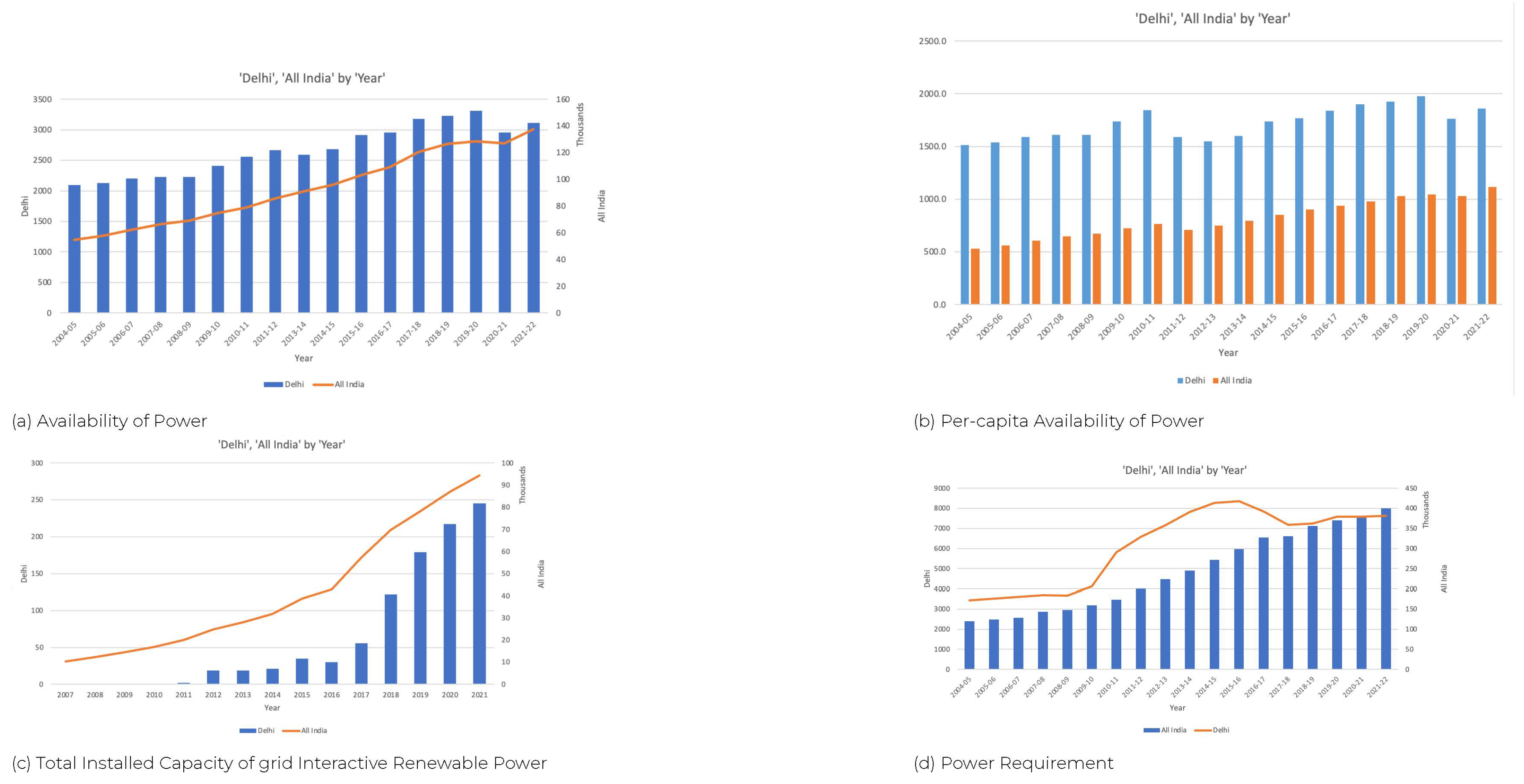
Figure 3. Analysis of Literature Survey Framework.

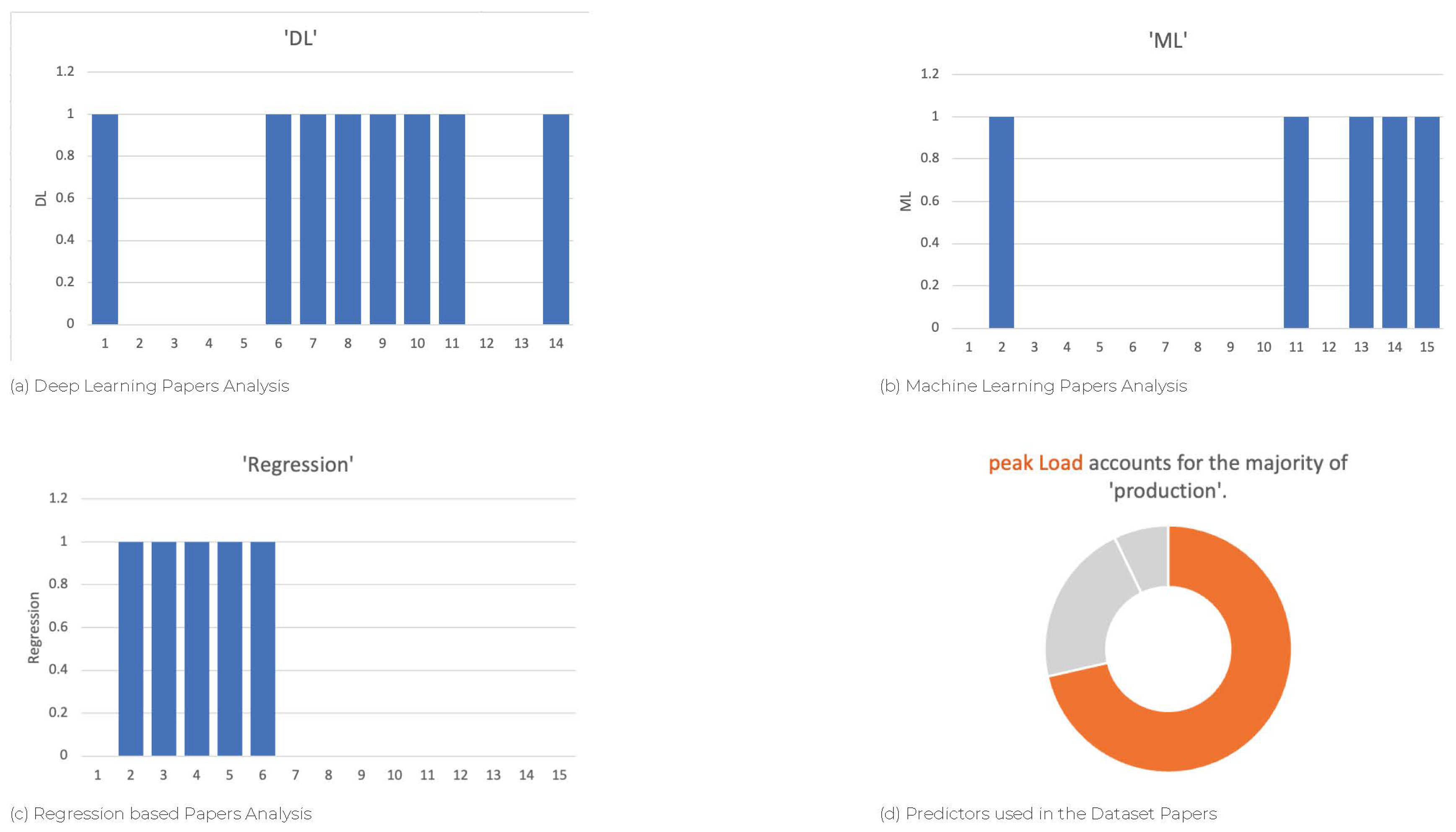
Table 1. Datasets names which are created from the reports.

1	dropna-dataset
2	mean Imputation dataset
3	median Imputation dataset
4	mode Imputation dataset
5	linear-Interpolation Imputation dataset

Table 2. ARIMA Model Comparison Results for dropna.

Models	Order	test_MAPE	train_MAPE	AIC	BIC
AR/MA models	1,0,0	19.483	26.125	50534.716	50553.290
	2,0,0	19.516	26.126	50534.362	50559.127
	1,1,0	21.903	26.602	50575.065	50587.447
	1,2,0	90.594	27.274	52837.437	52829.454
	0,0,1	16.617	21.619	56254.968	56273.542
	0,1,1	21.811	26.594	50572.554	50584.936
	0,2,1	21.9037	26.602	50578.459	50590.841
ARMA models	8,0,8	18.157	26.332	50067.375	50178.816
	8,1,8	18.814	26.453	50148.885	50254.131
	9,0,7	18.201	26.226	50067.729	50179.170
	9,1,7	18.332	26.453	50055.038	50160.283
	8,0,9	18.135	26.280	50068.705	50186.337
	8,1,9	18.274	26.464	50059.330	50170.766
auto-arima	5,1,3	18.844	26.454	50190.242	50245.961

Table 3. ARIMA Model Comparison Results for Mean Imputation.

Models	Order	test_MAPE	train_MAPE	AIC	BIC
AR/MA models	(1, 0, 0)	19.186	25.749	52184.042	52202.676
	(2, 0, 0)	19.352	25.756	52144.192	52169.037
	(1, 1, 0)	21.628	26.276	52188.319	52200.741
	(1, 2, 0)	86.037	27.046	54529.566	54542.004
	(0, 0, 1)	16.616	21.290	57600.735	57619.368
	(0, 1, 1)	21.322	26.248	52171.044	52183.466
	(0, 2, 1)	21.628	26.276	52243.646	52256.067
ARMA models	(9, 0, 8)	18.266	26.027	51635.298	51753.311
	(9, 1, 8)	18.069	26.135	51687.745	51799.541
	(8, 0, 9)	18.400	25.965	51663.391	51781.404
	(8, 1, 9)	18.366	26.173	51695.921	51807.718
	(8, 0, 8)	18.518	25.977	51670.186	51781.988
	(8, 1, 8)	18.324	26.093	51637.395	51742.981
auto-arima	(5, 1, 3)	18.563	26.085	51820.469	51876.368

Table 4. ARIMA model Comparison Results for Median Imputation.

Models	Order	test_MAPE	train_MAPE	AIC	BIC
AR/MA models	1,0,0	19.203	25.740	52180.550	52199.184
	2,0,0	19.363	25.748	52142.980	52167.825
	1,1,0	21.636	26.268	52187.390	52199.812
	1,2,0	86.201	27.038	54527.913	54540.351
	0,0,1	16.646	21.271	57600.941	57619.575
	0,1,1	21.336	26.241	52170.583	52183.005
	0,2,1	21.636	26.268	52239.944	52252.365
ARMA models	9,0,8	18.288	26.032	51635.740	51753.753
	9,1,8	18.115	26.121	51681.885	51793.682
	8,0,8	18.506	25.958	51674.400	51786.202
	8,1,8	18.421	26.104	51641.077	51746.663
	8,0,9	18.407	25.939	51668.680	51786.693
	8,1,9	18.502	26.152	51701.538	51813.335
auto-arima	5,1,3	18.676	26.098	51805.777	51861.675

Table 5. ARIMA model Comparison Results for Median Imputation.

Models	Order	test_MAPE	train_MAPE	AIC	BIC
AR/MA models	1,0,0	19.025	25.966	52851.514	52870.148
	2,0,0	19.256	25.977	52780.739	52805.583
	1,1,0	21.531	26.566	52831.433	52843.854
	1,2,0	85.088	27.498	55261.639	55274.078
	0,0,1	16.796	21.587	57849.604	57868.238
	0,1,1	21.013	26.513	52795.815	52808.237
	0,2,1	21.531	26.566	52925.747	52938.168
ARMA models	9,0,8	18.004	26.273	52357.307	52475.320
	9,1,8	22.428	26.522	52691.287	52803.084
	9,0,9	18.237	26.157	52376.970	52501.194
	9,1,9	16.651	26.512	52356.583	52474.591
	8,0,9	18.343	26.220	52412.001	52530.014
	8,1,9	18.698	26.342	52578.576	52690.373
auto-arima	3,1,4	18.401	26.340	52506.970	52562.869

Table 6. ARIMA model Comparison Results for Linear Interpolation Imputation.

Models	Order	test_MAPE	train_MAPE	AIC	BIC
AR/MA models	1,0,0	19.552	26.051	51429.997	51448.631
	2,0,0	19.573	26.051	51430.941	51455.786
	1,1,0	21.936	26.516	51472.149	51484.571
	1,2,0	90.903	27.171	53740.953	53753.391
	0,0,1	16.678	21.549	57337.414	57356.048
	0,1,1	21.870	26.510	51470.598	51483.020
	0,2,1	21.936	26.516	51473.203	51485.624
ARMA models	8,0,8	18.409	26.271	50801.251	50913.053
	8,1,8	18.683	26.385	50838.995	50944.581
	9,0,8	18.223	26.175	50814.366	50932.379
	9,1,8	18.440	26.385	50807.144	50918.941
	9,0,7	18.157	26.114	50836.848	50948.650
	9,1,7	19.432	26.363	50840.746	50946.332
auto-arima	5,1,4	19.114	26.389	51004.208	51066.318

Table 7. SARIMA model Comparison Results for dropna.

order	Seasonal-order	train_MAPE	test_MAPE	AIC	BIC
(1, 0, 0)	(3,0,6,7)	26.673	20.554	50233.507	50301.610
(0,0,0)	(1,0,1,7)	26.301	17.40	54957.193	54975.766
(0,0,0)	(1,1,1,7)	26.461	16.882	54823.939	54842.507
(0,0,0)	(3,0,6,7)	25.505	15.670	54736.140	54798.052
(0,0,0)	(3,1,6,7)	26.826	15.854	54735.359	54797.251

Table 8. SARIMA model Comparison Results for mean Imputation.

order	Seasonal-order	train_MAPE	test_MAPE	AIC	BIC
(1, 0, 0)	(6,0,2,7)	25.884	17.775	51748.896	51811.008
(0,0,0)	(1,0,1,7)	25.973	17.382	56160.584	56179.218
(0,0,0)	(1,1,1,7)	26.141	16.831	56026.752	56045.380
(0,0,0)	(6,0,2,7)	25.355	15.398	55932.485	55988.386
(0,0,0)	(6,1,2,7)	26.404	16.173	55954.966	56010.850

Table 9. SARIMA model Comparison Results for Median Imputation.

order	Seasonal-order	test_MAPE	train_MAPE	AIC	BIC
(1, 0, 0)	(3,0,6,7)	20.491	26.316	51825.927	51894.250
(0,0,0)	(1,0,1,7)	17.379	25.965	56152.138	56170.772
(0,0,0)	(1,1,1,7)	16.830	26.132	56018.390	56037.018
(0,0,0)	(3,0,6,7)	15.717	25.119	55924.073	55986.185
(0,0,0)	(3,1,6,7)	15.950	26.439	55951.882	56013.975

Table 10. SARIMA model Comparison Results for Mode Imputation.

order	Seasonal-order	test_MAPE	train_MAPE	AIC	BIC
(1, 0, 0)	(3,0,6,7)	20.554	26.673	50233.507	50301.610
(0,0,0)	(1,0,1,7)	17.407	26.301	54957.193	54975.766
(0,0,0)	(1,1,1,7)	16.882	26.461	54823.939	54842.507
(0,0,0)	(3,0,6,7)	15.670	25.505	54736.140	54798.052
(0,0,0)	(3,1,6,7)	15.854	26.826	54735.359	54797.251

Table 11. SARIMA Model Comparison Results for Linear Interpolation Imputation.

order	Seasonal-order	test_MAPE	train_MAPE	AIC	BIC
(1, 0, 0)	(6, 0, 3, 7)	19.905	26.556	50917.697	50986.020
(0, 0, 0)	(1, 0, 1, 7)	17.401	26.212	55984.215	56002.849
(0, 0, 0)	(1, 1, 1, 7)	16.871	26.372	55851.605	55870.233
(0, 0, 0)	(6, 0, 3, 7)	15.304	26.425	55773.403	55835.515
(0, 0, 0)	(6, 1, 3, 7)	15.210	26.442	55627.806	55689.899

Disclaimer/Publisher’s Note: The statements, opinions and data contained in all publications are solely those of the individual author(s) and contributor(s) and not of MDPI and/or the editor(s). MDPI and/or the editor(s) disclaim responsibility for any injury to people or property resulting from any ideas, methods, instructions or products referred to in the content.

© 2023 by the authors. Licensee MDPI, Basel, Switzerland. This article is an open access article distributed under the terms and conditions of the Creative Commons Attribution (CC BY) license (http://creativecommons.org/licenses/by/4.0/).

Copyright: This open access article is published under a Creative Commons CC BY 4.0 license, which permit the free download, distribution, and reuse, provided that the author and preprint are cited in any reuse.

PM-Gati Shakti: A Case Study of Demand Forecasting

Abstract

Keywords:

Subject:

Introduction

Delhi Yearly Power Statistics

Relation to Demand Forecasting

PM-Gati Scheme Initiative

Related Work

Deep Learning

Machine Learning

Regression Based Learning

Summary of Literature Survey

Data Overview

Forecasting Models

Datasets Analysis and ADF test results

Auto Regression and Moving Average model

Seasonal Auto-Regressive Models

Results and Conclusion

Acknowledgments

References

MDPI Initiatives

Important Links

Subscribe