
Submitted:
28 July 2023
Posted:
01 August 2023
You are already at the latest version
Abstract
Living beings are composite thermodynamic systems in non-equilibrium conditions. Within this context, there are a number of thermodynamic potential differences (forces) between them and the surroundings, as well as internally. These forces lead to flows, which, ultimately, are essential to life itself. Living beings are under the pressures of natural selection, thus are biological flows as well. At the same time, the maintenance of homeostatic conditions, the tenet of physiology, demands regulation of these flows by control of variables. However, due to the very nature of these systems, regulation of flows and control of variables become entangled in closed loops. Therefore, the search for adaptation in flows takes a different path than the search for adaptation in morphological traits. Being at the roots of transfer processes, thermodynamic criteria turn out to be as natural physical candidates. Likewise, being at the roots of physiology, control turns out to be as a natural biological candidate in that path. Here we show how to combine entropy generation, with respect to a generalized process, and control of parameters (in such a generalized process) in order to create a criterium of optimal ways to regulate changes in generalized flows.
Keywords:
entropy generation
; control
; elasticities
; flow
; optimality
; physiology
; biology
; thermodynamics
1. Introduction
Life is maintained by flows and it evolves by means of selective pressures. Thus, the flows, which encompass a wide range of biological phenomena from enzymatic reactions to population dynamics, are under the natural selection paradigm as well. Then, can we use a given flow as a criterion of selection? If so, which would such a criterion be?
Homeostasis, the maintenance of the organic internal media under adequate conditions [1], is the basic principle in physiology, and it is akin to cybernetics comprising information and control [2,3]. Therefore, at a very first glance, one would consider the control of a given flow as criterion of its relevance and thus how it was eventually shaped by natural selection. In the next two paragraphs, we shall exam why this cannot be an adequate criterion.
Flows are related to unbalanced forces and conductance properties of a system. For instance, the flow in the circulatory system can be written as:
where Jco is the cardiac output (the flow), XP is the pressure difference between the arterial and the venous trees (the unbalanced force) and Gper is the peripheral vascular conductance (the inverse of the peripheral resistance). From the control engineering standpoint, the cardiac output is a regulated variable while the pressure difference and the conductance are controlled variables [4,5]. In this sense, pressure and conductance are directly under a certain policy rule to regulate the flow, which is not directly accessed by the controlling system.
However, both pressure and conductance are, at a second level, controlled variables on their own, since they are regulated by a series of underlying mechanisms. For instance, among other variables, arteriolar wall muscle tone regulates peripheral conductance and myocardial contraction force regulates arterial pressure (e.g. [6,7,8]). The control of these muscles occurs at a cellular level, and then, they become controlled variables at a third level, and these nested levels of regulation/control will proceed to a number of steps. Because they operate basically in closed control loops among the levels, to try to identify or isolate the “fundamental controlling variables” becomes a search for the holy grail: from one perspective, a given variable is regulated while it is controlled from another (Figure 1). Therefore, the search for adaptation in flows is of a different kind than the search for adaptation in morphological traits.
2. Flows and Optimization
We can identify that this search for optimization criteria in flows has three strands: the phylogenetic, the ontogenetic and the adjustment (phenotypic plasticity) levels. Despite closely related, these levels might not be imbricate in each other in a variety of circumstances. From these strands, the most prominent is the phylogenetic search for optimization since this is the level where natural selection emerges more clearly (e.g., [11,12]). This reasoning, however, might be accompanied by a pitfall. Since adaptation is a continuous process, the search relies on finding local minima or maxima and not global optima [13]. This means that different species might seem to behave differently under the same criterion.
Then, what would be an adequate non ad hoc criterion to the optimization of a given biological flow? From the preceding discussion, one would suppose that the process generating the flow is under its way to a local maximum or minimum, but it is close enough to the local extremum to be clearly identified. Once again, an inference must be made: the organism passes most of its time under a certain value of the flow in focus; otherwise, it makes no sense in considering the value of the flow as a selected variable.
From the last paragraph, we can see some problems that hinder the search for optimality criteria in biological flows. Because the extremum is local and one cannot say whether it is already attained or not, and because time must be taken into account, one risks becoming tautological: it is optimum because it is what one observes.
On the other hand, a predetermined criterion might partially circumvent this tautological pitfall. Historically, this predetermined criterion comes from the energetic bias. Power input to and/or power output from a given process (flow) are employed to address the quest for optimization. The success of such an approach is so widespread that it would be impossible to summarize its results in this review (see, for instance, [14,15]).
3. Thermodynamic Criteria for Optimization
The energetic bias has a crucial aspect. Arising from thermodynamic grounds, it offers a lower risk of a tautological criterion for extrema, and it also offers limitations to extrema as well. However, as one might suspect, pitfalls are lurking every now and then.
Let us consider hibernation in mammals. Many hibernators spend months under the torpid condition, and depending on the species and the surrounding environment, this may last for most of the year (e.g., [16,17]). Therefore, combining extreme low metabolic values with the “time under a condition” criterion, torpid metabolic rate would be the flow under selection, and not basal or resting metabolic rate as we would expect and consider as for other species [15,18,19,20,21,22]. This example illustrates that to interpret the selection acting on biological flows is potentially deceitful.
Evidently, the reproductive success is paramount to evolution, and, from this perspective, the measure of its selective advantage is the prevalence of a given genome in the population (e.g., [23,24]). In this sense, the torpid condition of the above example certainly contributes to the reproductive success of the species, but reproduction per se does not occur in the torpid condition. And by the genomic bias, all optimizations of physiological processes become tautological: they are what is measured in the population that has been selected.
Given this very intricate picture, can we find another way to approach some features of physiological and biological flows in general that might help us understanding the evolutionary pressure or its consequences over a given flow?
4. The Present Approach to Optimization
We propose that instead of looking directly to a given flow from any given bias, one asks whether the regulation of this flow follows an optimal path. In other words, when a given flow Ji(A) of a process “i" under condition “A” is lead to Ji(B) under condition “B”, does this follows an optimal path? Note that we are not asking whether Ji(A) or Ji(B), or both, are extrema. We are concerned in how optimal the transition between conditions is.
Then, how to establish what is an optimum path? Certainly, thermodynamic criteria are the best choices for a series of reasons. Firstly, they are prone to be quantified and we unambiguously know what is meant by efficiency in this frame. Secondly, one way or the other, they rule the time evolution of non-biological systems and, thus, living beings inherit such an unescapable realm. Thirdly, classical thermodynamics begins with clear definitions of what is the system under study and, consequently, what are the surroundings. Finally, flows are generated by thermodynamic potentials and, thus, it becomes quite natural and pervasive to consider thermodynamic criteria as the best choice to study selection in physiological flows.
Let us consider flows in general. In conditions near equilibrium, a flow J is the product of an unbalanced force or potential difference X by a conductance G as [25,26]. As for the equation for cardiac output presented in the beginning, we have:
An essential feature of a thermodynamic flows is that they tend to extinguish unbalanced forces and, therefore, they tend to extinguish themselves. In other words, after a certain characteristic time which depends on the conductance G, X → 0 and J → 0. Thus, if nothing else occurs, the system tends to equilibrium. Likewise, in order to keep a flow at a given rate, unbalanced forces must be sustained.
Now, if the system is left to evolve without any other agent at play, the extinction of the unbalanced force X equates to the loss of capacity to perform useful work by the system, i.e., a decrease in its free energy and an increase in its entropy [27,28,29]. For instance, let us briefly exam the loss of useful work in the isothermal diffusive process. Variation in Gibbs free energy, dGibbs, is given as:
where V is volume, P is pressure, S is entropy and T is temperature. Given the isothermal condition, dT = 0, and rearranging the ideal gas equation, we have:
where n is the number of mols, C is the concentration and R is the universal gas constant. Thus, the loss in useful work due to the diffusive flow equating the initial concentration in the system to the concentration in the infinite pool of the surroundings is:
where, for the sake of simplicity and without any loss of generality, we consider Cfinal < Cinitial. This equates, then, with the entropy increase as . On the other hand, if the initial concentration in the system is kept constant despite the outflow of molecules, then the time derivative of the lost work is the lost useful power in the system:
where C2 and C1 are fixed values. Note that is the flow of molecules and the rest of the equation to its right side is the chemical potential. From this example we now proceed to generalizations.
4.1. Entropy Generation
An important branch of contemporary thermodynamics is exergetic analysis, which combines the 1st and the 2nd Laws of thermodynamics into a single approach [28,29,30]. In this approach, it is considered the maximum useful work that can be extracted from a system when it is lead, reversibly, to the ground state, i.e., it attains mechanical, thermal, and chemical equilibrium with the surroundings through reversible paths. If the system experiences irreversible processes, entropy generation by these processes decreases the exergetic efficiency by destroying exergy, which corresponds to a degradation of the surroundings. Considering that in living beings the basic source of energy input is a decrease of Gibbs’ free energy from combustibles (basically glucose and similar sugars), there is a high degree of coincidence between the energetic and the exergetic analyses (Silvio de Oliveira Junior and Carlos Eduardo Mady personal communication). In face of this wide picture, we shall focus in entropy generation.
For the sake of notation, we are omitting the subscript “i” referring to each process in the system. Also, for simplicity, we shall not be concerned with the coupling between potentials, as in the electrochemical potential.
As one can see, the entropy generation is a direct measure of how much the system degrades its surroundings in order to keep a given flow that sustains life. Or, alternatively, σ is related to the non-efficiency of a system in keeping a given flow. Therefore, even though less comprehensive than the exergetic approach, this is as well an appropriate thermodynamic criterion for analyses (see, also, [32,33]).
4.2. Coefficients of Control
As we stated earlier, both X and G can be studied as controlled variables. Consider a set of parameters K = {k1, k2 … kn} in such a way that, for a given process “i”:
Consider a certain parameter ka ∈ K. Then, flow regulation by the parameter ka implies in:
And the relative variation (i.e., elasticity) of flow is:
For historical reasons, the elasticity is named “flux control coefficient” (by the parameter ka) [34,35,36,37,38]:
Applying the elasticity concept to the entropy generation (Equation (2)), one obtains (we omit the intermediate algebra):
Then, combining Equations (6) and (7), we obtain a new coefficient of elasticity associating relative changes in flow to relative changes in entropy generation when there is a variation in the parameter ka:
And we name this new quantity as flow-entropy coefficient. It must be understood that the flow-entropy coefficient is a value related to changes in a given parameter ka of the system and that it is in respect to a certain process (or flow). Taking for granted that these are implied in the notation, we simplify the flow-entropy coefficient to:
Now, there is a term whose meaning must be clarified before we proceed. As we stated earlier, the system and, consequently, the surroundings are to be defined at the beginning of the analysis. Therefore, one might consider the surroundings’ temperature as the reference, and then, each process “i" contributes with its σi in the total entropy generation of the system as a non-reversible heat loss to the surroundings. In a vast number of cases, within the time scale of the changes in a given flow, the surroundings can be taken as an infinite pool and, thus, one can consider for the purposes of the analysis. This will be assumed in the remaining of the present text, except in the working example at the end. Then, Equation (8) becomes:
where it is understood that the elasticities are related to some parameter ka.
A last thing must be said before we continue. Elasticities, and therefore control coefficients, are non-dimensional quantities, i.e., they are pure numbers. When computing a given coefficient, it is important to check out if the resulting value is a pure number since these computations might become quite demanding in some cases.
4.3. The values of
For sure, the next question in mind is how Equation (10), i.e., the flow-entropy coefficient , can be of any help. The answer to this question is quite clear: The lower the value of the more a flow can be increased relative to the entropy generation of the process. In other words, lower values indicate optimal paths to increase a given flow.
From the preceding paragraph, one would conjecture that, then, to obtain an increase in flow along with a decrease in entropy generation is “the best of both worlds”. That is, paths that have are the best choices. Let us exam Equation (4) and ask how a positive change (i.e., an increase) in flow might be brought about. Rewriting Equation (4) as a positive change in flow, we have:
Developing the term between parenthesis:
We now exam a decrease in entropy generation:
Developing the term between parenthesis:axis as a graphical representation of the solutions of inequations
Thus:
Both X and G are, from our perspective, positive values.
Figure 2 illustrates the conditions for increase in flow and decrease in entropy generation (inequations (11b) and (12c), respectively) due to changes in conductance and force. As it can be seen, “the best of both worlds” can be obtained only in narrow band of a few situations where and , and such an existence depends on the actual values of X and G themselves. In other words, it is possible to obtain an increase in flow with a decrease in entropy generation depending on the values of the potential difference and the conductance if the conductance increases while the force decreases. This corresponds to .
However, care must be taken when a is found. Notice that “the worst of both worlds” also lurks in the way, since paths in which may indicate that a flow decreases while its entropy generation increases.
The preceding discussion focused on increases of a given flow. What if the flow is to be decreased? Then, we have the specular image of what happens in the increase zone: the higher the value the better the path. This is easy to understand if one considers while dJ < 0. In this situation, the system still deals with the same amount of lost work but has a lower flow rate. Figure 3 summarizes these various situations depicted so far in reference to Equation (10). It is essential to note that for each parameter ka, the associated value is a single point in the vs plane. Alternatively, if turns out as a function of the parameter, then it might assume different values along the changes in ka. In the final section of the present manuscript, we develop a case study of this last type.
4.4. and Physiological Adjustments
We turn, now, to another facet of the flow-entropy coefficient. Given the natural selection process, one can conjecture that an organism operating under a given condition has a set of parameters and variables that assume their same respective values whenever the system is in that given condition. This is what makes it possible to compare different individuals and a single individual in different conditions.
Consider the system at a given condition A and then it transits to another condition B. Both A and B have specified demands (i.e., a given flow) for a given condition, for example, transition from rest to a moderate level of physical effort, or a temperature change in the surroundings that puts the animal bellow its thermoneutral zone. Let us assume that the transition is brought about by an increase in parameter ka, and that the associated coefficient is . From Figure 3 we can see that this is a fairly good value representing an increase of 0.8 unities of entropy production for each unit of increase in the flow, that is, the proportional increase in entropy generation falls below the increase in flow. Then, the system returns to condition A, decreasing the parameter ka. Since is the same, the returning path also has a decrease in entropy generation that falls behind the decrease in flow. That is, while in the first transition the system obtained an advantage in terms of the relationship between increase in flow and increase in entropy generation, in the returning transition the system has a disadvantage in the decrease in flow and the decrease in entropy generation.
In other words, one would like to minimize when a given flow is increased, but to maximize when a given flow is decreased. However, because is a single function for a parameter ka, this is not possible. In terms of phylogenetic evolution and ontogenetic development this is not a problem since these are one-way paths that once traveled would be no return. However, for physiological adjustments, the picture is quite different because they are two-way roads.
Therefore, it would be expected that optimized physiological adjustments operate transitions in one of two modes. The first is to have , and then, changes in flow have a low impact in entropy generation one way or the other. Appealing as such a solution might seem, thermodynamic constraints impose severe limits to this option. The second mode is to have hysteresis in the process. For instance, instead of transitions as A → B → A, one performs A → B’ → B → A’ → A. While in the final conditions A and B the parameter ka attains specified values, the intermediate conditions B’ and A’ comprise changes through other parameters that allow for a hysteresis in the cycle. Then, as in the Carnot cycle, the area enclosed by the path represents a net gain in terms of entropy generation in relation to changes in flow.
For the sake of concreteness, let us give an example of a hysteresis in flow, in this case, metabolic rate (i.e., oxygen consumption rate). Figure 4 illustrates a schematic representation of the entry to and arousal from a torpor episode by a heterothermic endotherm, as a small mammal in temperate climates. As it can be seen in the plot, the arousal is not a mirror image of the entry phase. Then, one could ask whether there is an optimization in entropy generation due to this hysteresis in the process. This is the kind of question that the flow-entropy coefficient tries to answer when dealing with physiological adjustments.
5. A working Example
A more profound analysis of how to employ the flow-entropy coefficient in the phylogenetic domain is presented elsewhere, and there we show the reasons for the observed scaling of blood pressure and volume [32]. Presently, we opted to take a different bias, now in the populational domain, in order to show the broadness of the method analyzing vaccination effort as control parameter of a contagious disease. The model we use is the common SIR (Susceptible, Infected, Recovered) model plus the vaccinated V state, or the SIRV model (e.g. [41,42]). The present analysis is not intended to bring changes in the current understanding of this model, but to show an alternative way of interpreting the results. The model is given by four differential equations:
where P is the birth rate of the population, a is the transmissibility or infective constant rate, v is the vaccination constant rate (vaccination effort), μ is the mortality rate for the population in general, r is the recovery from the disease constant rate and m is the mortality constant rate from the disease. Without loss of generality, in this example the total population is not kept constant.
For the sake of notation, let
The equilibrium point of the system (13) for the endemic case (i.e., ) is obtained from the second equation of the system, and we have:
where the superscript “*” is to indicate the value of the state variable at the equilibrium point.
From Equation (15), which represents the endemic case, the infected population becomes:
From Equation (16) we can identify a critical value of vaccination effort that eradicates the disease (i.e., ):
Thus, we examine the model within the range:
Now, we define the generalized flow J as the rate of people becoming infected:
where a becomes the generalized conductance G and the product acts as the generalized force. From Equations (15) and (16), Equation (18) becomes:
Let us conceive a suitable “temperature” for this system as:
where H is a normalized number related to per capita income of the given population and z is a constant that relates a decrease in per capita income to the number of infected people . Therefore, the generalized entropy generation is a measure of how the spreading of the infectious disease impacts the society, and its equation becomes:
To study the effect of vaccination effort in the system, we start by computing the following partial derivatives:
Here, we omit the intermediate algebra and present the results straightway:
For completeness of the working example, let us check out whether these coefficients are pure numbers. The dimensions involved are [n], number of people, and [t], time. The dimensions of the parameters are presented in Table 1.
Thus, the flow J has dimension of [n t-1] and the coefficients are non-dimensional quantities, indeed.
is a function of v, negative in this case, indicating that an increase in vaccination effort causes a decrease in infection flow (as expected). Notice that and . This is a quite interesting result indicating that as the vaccination effort increases it gains further control over disease flow, while for v ≅ 0 vaccination effort offers little control over infection flow in the population.
Notice that is also a function of v, and thus it is not a single point in the CG vs CX plane (Figure 3): if v = 0, while if v = vcrit, . The positiveness of indicates that if the flow increases (due to a reduction in vaccination effort, see above) the generalized entropy generation, i.e., the negative impact over society, increases as well (and vice-versa). Notice, also, that for all v, meaning that the vaccination effort causes a disproportional greater change in generalized entropy generation in relation to disease flow. However, in this case, the result is beneficial, since we are interested in decreasing the impact of the disease in society (i.e., we are in the light grey area of Figure 3). Figure 5 shows the plots of and of as functions of vaccination effort.
It is important to note that the approach we exemplify here using v = ka can be done for any of the parameters of the model, namely, P, a, μ, r, m, z. As previously mentioned, we do not intend to create a new model of vaccination, and neither to analyze the model in terms of its equilibrium points and their respective stability or conditions to eliminate the contagious disease. Instead, our intention is to show an alternative way to interpret the impact of the parameters in the dynamics of the disease. In the light of this, the coefficients of elasticity are a powerful tool to elucidate relationships between the parameters of the model and concepts such as efficacy, efficiency, optimization, etc.
Author Contributions
Conceptualization, J.G.C.-B.; methodology, J.G.C.-B., J.E.P.W.B.; validation, J.G.C.-B, P.G.N.-d.-S.; formal analysis, J.G.C.-B., J.E.P.W.B., P.G.N.-d.-S.; writing—original draft preparation, J.G.C.-B., J.E.P.W.B., P.G.N-S.; writing— J.G.C.-B., J.E.P.W.B., P.G.N.-d.-S. All authors have read and agreed to the published version of the manuscript.
Funding
This study had no fundings.
Data Availability Statement
There is no new data in this study.
Acknowledgments
The authors thank the random chance of being together.
Conflicts of Interest
The authors declare no conflict of interest.
References
- Cannon, W.B. Organization for physiological homeostasis. Physiol Rev. 1929, 9, 399–431. [Google Scholar] [CrossRef]
- Billman, G.E. Homeostasis: The Underappreciated and Far Too Often Ignored Central Organizing Principle of Physiology. Front Physiol. 2020, 11, 1–12. [Google Scholar] [CrossRef]
- Goldstein, D.S. How does homeostasis happen? Integrative physiological, systems biological, and evolutionary perspectives. Am J Physiol Regul Integr Comp Physiol. 2019, 316, R301–R317. [Google Scholar] [CrossRef] [PubMed]
- Windhorst, U. Regulatory Principles in Physiology. Comprehensive Human Physiology; Springer Berlin Heidelberg: Berlin, Heidelberg, 1996; pp. 21–42. [Google Scholar] [CrossRef]
- Nise, N. Control Systems Engineering, 3rd ed.; John Wiley & Sons, Inc.: New York, 2000. [Google Scholar]
- Levy, M.N.; Pappano, A.J. Cardiovascular physiology, 9th ed.; Mosby-Elsevier: Philadelphia, 2007. [Google Scholar]
- Chaui-Berlinck, J.G.; Monteiro, L.H.A. Frank-Starling mechanism and short-term adjustment of cardiac flow. J Exp Biol. 2017, 220, 4391–4398. [Google Scholar] [CrossRef] [PubMed]
- Solaro, R.J. Mechanisms of the Frank-Starling Law of the Heart: The Beat Goes On. Biophys J. 2007, 93, 4095–4096. [Google Scholar] [CrossRef] [PubMed]
- Mcentire, K.D.; Gage, M.; Gawne, R.; Hadfield, M.G.; Hulshof, C.; Johnson, M.A.; et al. Understanding Drivers of Variation and Predicting Variability Across Levels of Biological Organization. Integr Comp Biol. 2021, 61, 2119–2131. [Google Scholar] [CrossRef]
- Wade, M.J.; Kalisz, S. The causes of natural selection. Evolution (N Y). 1990, 44, 1947–1955. [Google Scholar] [CrossRef]
- Tibell, L.A.E.; Harms, U. Biological Principles and Threshold Concepts for Understanding Natural Selection: Implications for Developing Visualizations as a Pedagogic Tool. Sci Educ. 2017, 26, 953–973. [Google Scholar] [CrossRef]
- Wade, M.J. Constraints on Sexual Selection. Science 2012, 338, 749–750. [Google Scholar] [CrossRef]
- Barton, N.; Partridge, L. Limits to natural selection. BioEssays 2000, 22, 1075–1084. [Google Scholar] [CrossRef]
- Saadat, N.P.; Nies, T.; Rousset, Y.; Ebenhö, O. Thermodynamic limits and optimality of microbial growth. Entropy 2020, 22, 277. [Google Scholar] [CrossRef] [PubMed]
- Swanson, D.L.; McKechnie, A.E.; Vézina, F. How low can you go? An adaptive energetic framework for interpreting basal metabolic rate variation in endotherms. J Comp Physiol B Biochem Syst Environ Physiol. 2017, 187, 1039–1056. [Google Scholar] [CrossRef] [PubMed]
- Heldmaier, G.; Ortmann, S.; Elvert, R. Natural hypometabolism during hibernation and daily torpor in mammals. Respir Physiol Neurobiol. 2004, 141, 317–329. [Google Scholar] [CrossRef] [PubMed]
- Ruf, T.; Geiser, F. Daily torpor and hibernation in birds and mammals. Biol Rev. 2015, 90, 891–926. [Google Scholar] [CrossRef] [PubMed]
- Boratyński, Z.; Koteja, P. Sexual and natural selection on body mass and metabolic rates in free-living bank voles. Funct Ecol. 2010, 24, 1252–1261. [Google Scholar] [CrossRef]
- Burton, T.; Killen, S.S.; Armstrong, J.D.; Metcalfe, N.B. What causes intraspecific variation in resting metabolic rate and what are its ecological consequences? Proc R Soc B Biol Sci. 2011, 278, 3465–3473. [Google Scholar] [CrossRef]
- Rønning, B.; Moe, B.; Bech, C. Long-term repeatability makes basal metabolic rate a likely heritable trait in the zebra finch Taeniopygia guttata. J Exp Biol. 2005, 208, 4663–4669. [Google Scholar] [CrossRef]
- White, C.R.; Kearney, M.R. Determinants of inter-specific variation in basal metabolic rate. J Comp Physiol B. 2013, 183, 1–26. [Google Scholar] [CrossRef]
- Baškiera, S.; Gvoždík, L. Repeatability and heritability of resting metabolic rate in a long-lived amphibian. Comp Biochem Physiol Part A Mol Integr Physiol. 2021, 253, 110858. [Google Scholar] [CrossRef]
- Ellegren, H. Comparative genomics and the study of evolution by natural selection. Mol Ecol. 2008, 17, 4586–4596. [Google Scholar] [CrossRef]
- Bamshad, M.; Wooding, S.P. Signatures of natural selection in the human genome. Nat Rev Genet. 2003, 4, 99–111. [Google Scholar] [CrossRef]
- de Groot, S.R.; Mazur, P. Non-Equilibrium Thermodynamics; Dover unab; Dover Publications: Mineola, TX, USA, 1984. [Google Scholar]
- Lucia, U.; Grazzini, G. The second law today: Using maximum-minimum entropy generation. Entropy 2015, 17, 7786–7797. [Google Scholar] [CrossRef]
- Lucia, U. Entropy generation: Minimum inside and maximum outside. Phys A Stat Mech its Appl. 2014, 396, 61–65. [Google Scholar] [CrossRef]
- Bejan, A. Fundamentals of exergy analysis, entropy generation minimization, and the generation of flow architecture. Int J Energy Res. 2002, 26, 545–565. [Google Scholar] [CrossRef]
- Henriques, I.B.; Mady, C.E.K.; de Oliveira Junior, S. Exergy model of the human heart. Energy 2016, 117, 612–619. [Google Scholar] [CrossRef]
- Yildiz, C.; Bilgin, V.A.; Yılmaz, B.; Özilgen, M. Organisms live at far-from-equilibrium with their surroundings while maintaining homeostasis, importing exergy and exporting entropy. Int J Exergy. 2020, 31, 287–301. [Google Scholar] [CrossRef]
- Glansdorff, P.; Prigogine, I. Structure, Stabilité et Fluctuations; Masson & Cie Éditeurs: Paris, 1971. [Google Scholar]
- Chaui-Berlinck, J.G.; Bicudo, J.E.P.W. The Scaling of Blood Pressure and Volume. Foundations 2021, 1, 145–154. [Google Scholar] [CrossRef]
- Lucia, U.; Sciubba, E. From Lotka to the entropy generation approach. Phys A Stat Mech its Appl. 2013, 392, 3634–3639. [Google Scholar] [CrossRef]
- Visser, D.; Heijnen, J.J. The mathematics of Metabolic Control Analysis revisited. Metab Eng. 2002, 4, 114–123. [Google Scholar] [CrossRef]
- Reder, C. Metabolic control theory: A structural approach. J Theor Biol. 1988, 135, 175–201. [Google Scholar] [CrossRef]
- Giersch, C. Control analysis of metabolic networks. 1. Homogeneous functions and the summation theorems for control coefficients. Eur J Biochem. 1988, 174, 509–513. [Google Scholar] [CrossRef] [PubMed]
- Kacser, H.; Burns, J.A. The control of flux. Symp Soc Exp Biol. 1973, 27, 65–104. [Google Scholar] [CrossRef] [PubMed]
- Kacser, H.; Burns, J.A. Molecular Democracy: Who Shares the Controls? Biochem Soc Trans. 1979, 7, 1149–1160. [Google Scholar] [CrossRef] [PubMed]
- Nogueira de Sá, P.G.; Chaui-Berlinck, J.G. A thermodynamic-based approach to model the entry into metabolic depression by mammals and birds. J Comp Physiol B. 2022, 192, 593–610. [Google Scholar] [CrossRef] [PubMed]
- Nogueira-de-Sá, P.G.; Bicudo, J.E.P.W.; Chaui-Berlinck, J.G. Energy and time optimization during exit from torpor in vertebrate endotherms. J Comp Physiol B. 2023; on-line. [Google Scholar] [CrossRef]
- Batistela, C.M.; Correa, D.P.F.; Bueno, Á.M.; Piqueira, J.R.C. SIRSi-vaccine dynamical model for the COVID-19 pandemic. ISA Trans. 2023. [Google Scholar] [CrossRef]
- Harari, G.S.; Monteiro, L.H.A. A note on the impact of a behavioral side-effect of vaccine failure on the spread of a contagious disease. Ecol Complex. 2021, 46, 100929. [Google Scholar] [CrossRef]
Figure 1.
A general picture of levels of biological regulation/control. While the reductionist view would consider the upward processes at the left-hand side of the scheme as the mandatory in controlling flows, the downward closed loops shown in the right-hand side create an entanglement between levels of biological organization that somehow precludes a simple cut-off of what is a controlled and what is a regulated variable (see, for instance, [9,10]). This is valid within the organism and among organisms as well, since the biotic and abiotic environments would also dictate access to resources.
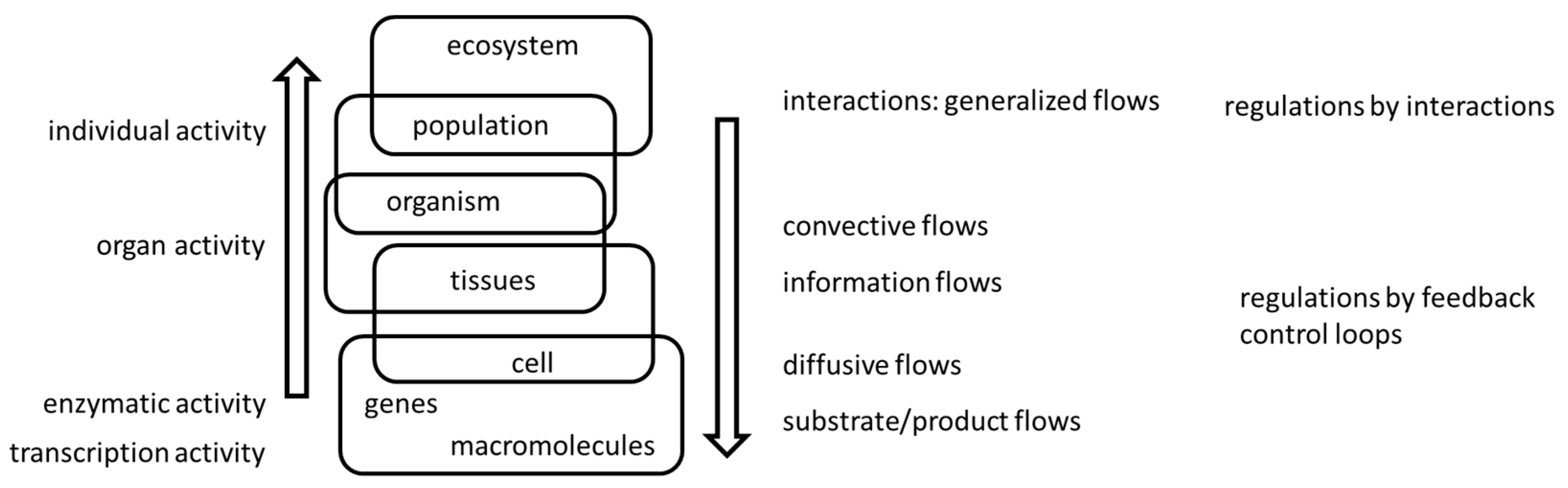
Figure 2.
axis as a graphical representation of the solutions of inequations (11b) and (12c). The solutions pertaining to each inequation are indicated by cross hatched bands. As it is shown, a simultaneous solution to both inequations is possible only if and . The upper line is for the case while the lower line is for the case . |⋅| indicates the absolute value.
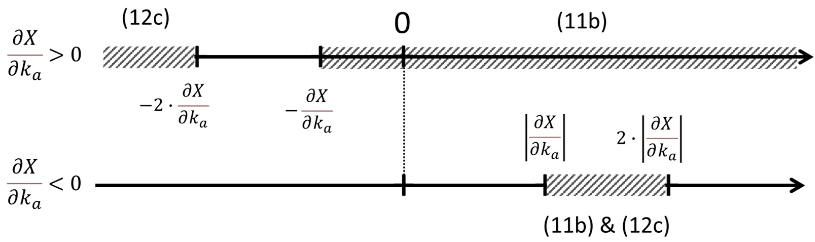
Figure 3.
The CG vs CX plane. The elasticities’ coefficients of the conductance G and of the potential X are represented as orthogonal axes. The dashed line corresponds to CG = -CX and the dotted-dashed line corresponds to CG = -2CX. These two lines form the boundaries of the “best of both worlds” (bbw) condition of dJ > 0 along with dσ < 0, and of the “worst of two worlds” (wbw) condition of dJ < 0 along with dσ > 0. In the outside zones there are two grey areas, one indicating the region with dJ > 0 and dσ > 0 (dark grey) and the other indicating the region with dJ < 0 and dσ < 0 (light grey). Both these regions have non-negative . However, in the former (dark grey zone), processes which occur in the 2nd quadrant are the most efficient, and processes which occur in the 4th quadrant are the most inefficient, while is the opposite in the latter (light grey zone). The 1st and the 3rd quadrants are of intermediate efficiencies in their respective zones. Numbers in parenthesis indicate the value over the respective line. For instance, along the CX axis, , while along the CG axis, . These results come immediately from Equation (10) since walk over one of these axes means to have no changes in the other.
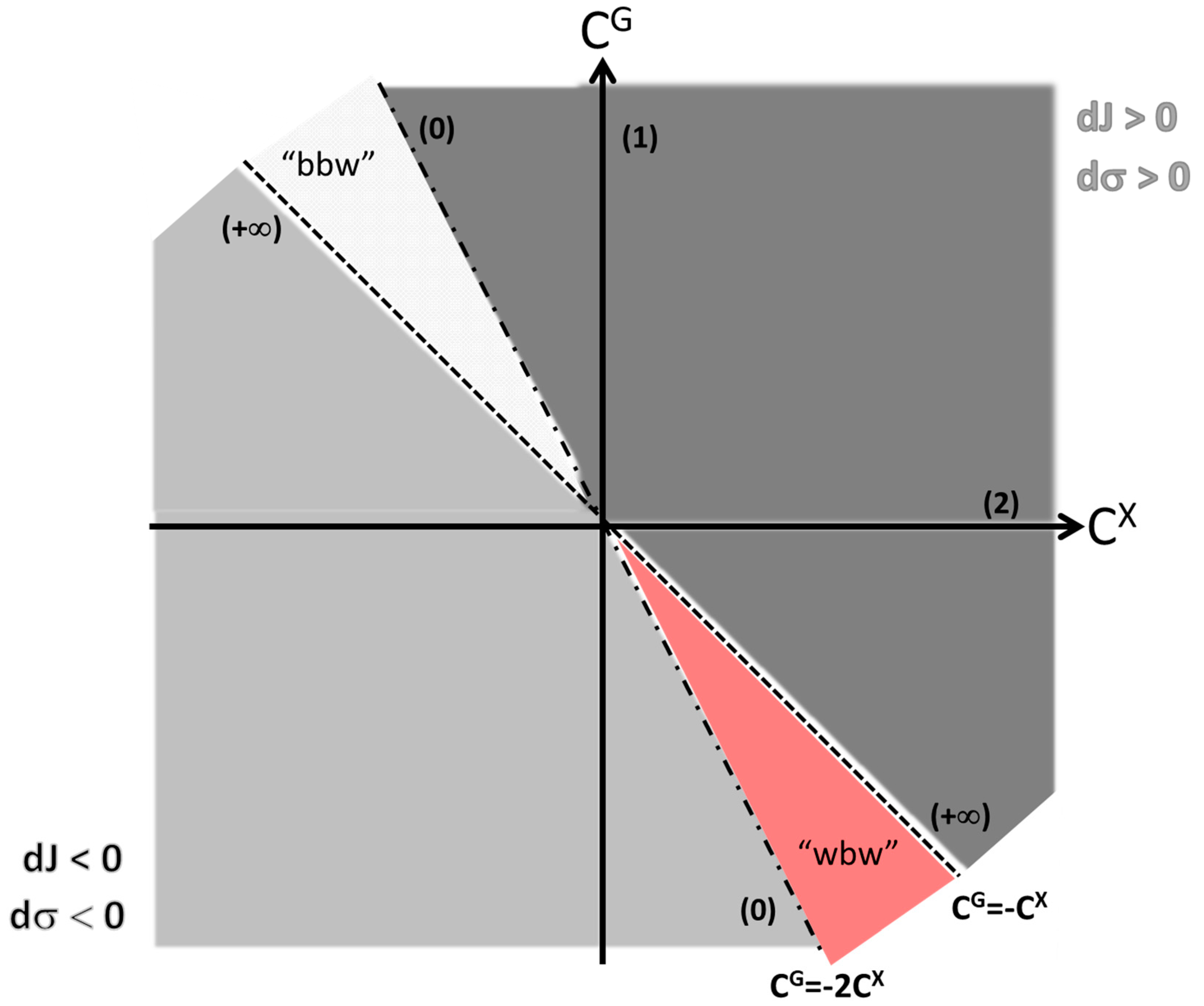
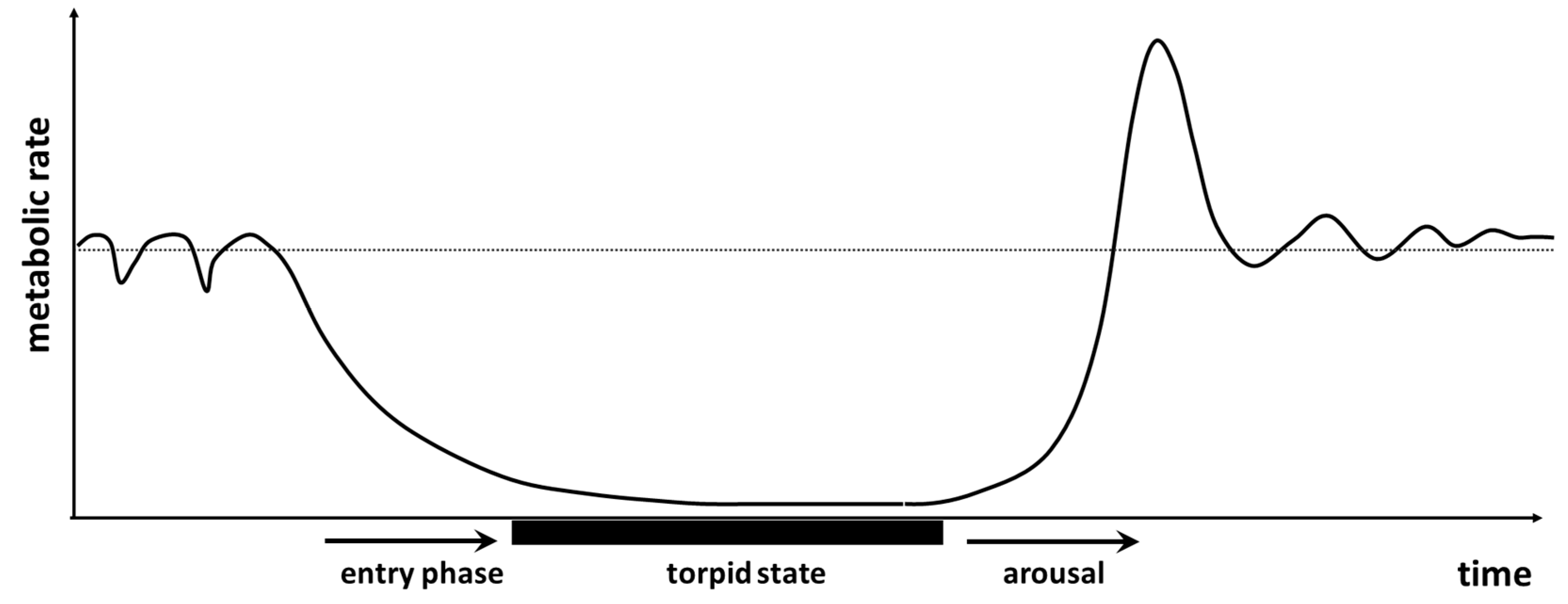
Figure 5.
(red) and (blue) versus vaccination effort. See text for detailed discussion.
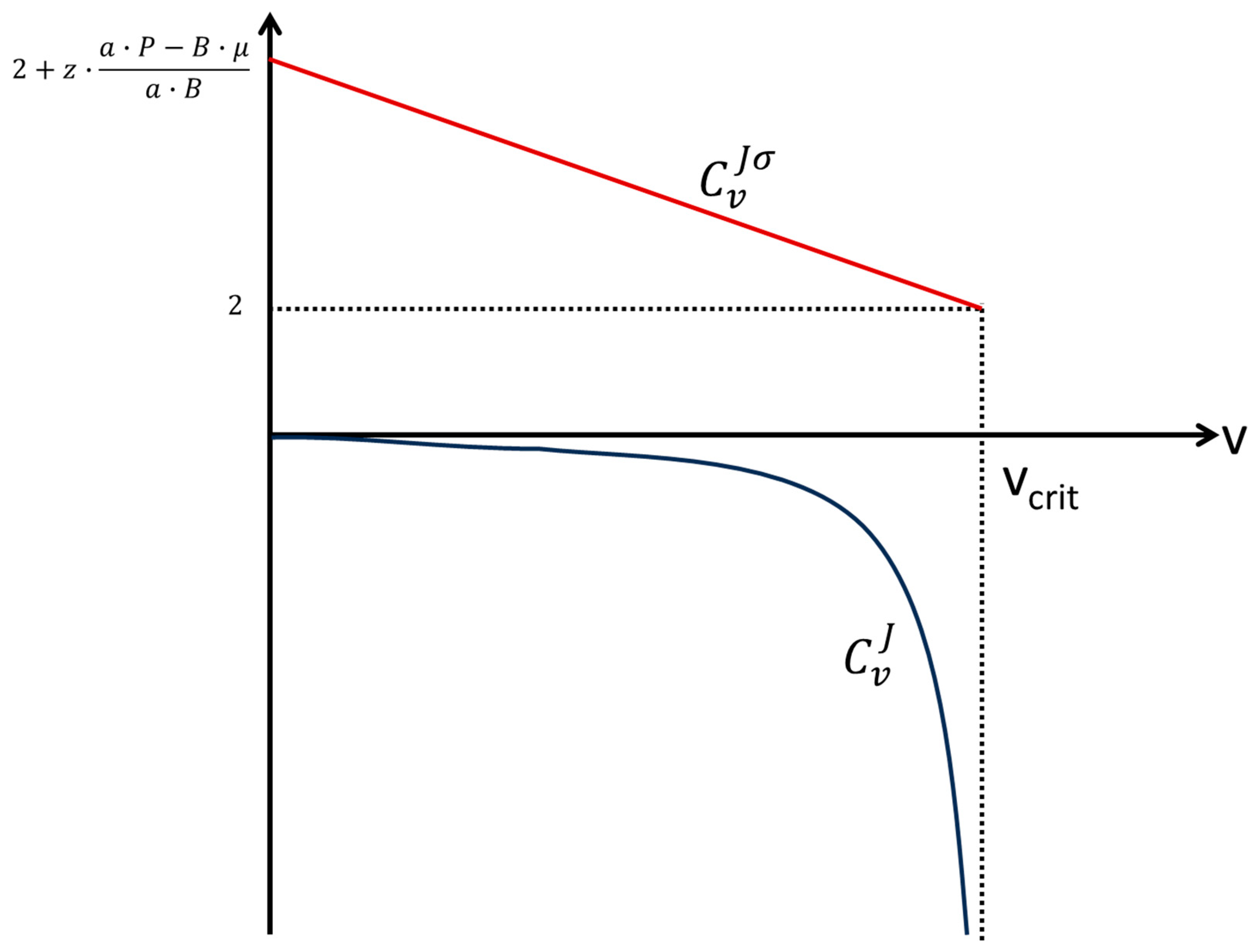

Table 1.
Dimension of the parameters in system (13).
| Parameter | Dimension |
|---|---|
| P | [n t-1] |
| a | [n-1 t-1] |
| B | [t-1] |
| v | [t-1] |
| z | [n-1] |
Disclaimer/Publisher’s Note: The statements, opinions and data contained in all publications are solely those of the individual author(s) and contributor(s) and not of MDPI and/or the editor(s). MDPI and/or the editor(s) disclaim responsibility for any injury to people or property resulting from any ideas, methods, instructions or products referred to in the content. |
© 2023 by the authors. Licensee MDPI, Basel, Switzerland. This article is an open access article distributed under the terms and conditions of the Creative Commons Attribution (CC BY) license (http://creativecommons.org/licenses/by/4.0/).
Copyright: This open access article is published under a Creative Commons CC BY 4.0 license, which permit the free download, distribution, and reuse, provided that the author and preprint are cited in any reuse.


