
Submitted:
31 July 2023
Posted:
01 August 2023
You are already at the latest version
Abstract
This paper deals with the viscoelastic behavior during crystallization and melting of semicrystalline polymers with the aim of later modeling the residual stresses after processing in case where crystallization occurs in quasi static conditions (in additive manufacturing for example). Despite of an abundant literature on polymer crystallization, the current state of scientific knowledge does not yet allow ab initio modeling. Therefore, an alternative and pragmatic way has been explored to propose a first approximation of the impact of crystallization and melting on the storage and the loss moduli during crystallization-melting-crystallization cycle. An experimental approach, combining DSC, optical microscopy and oscillatory shear rheology was used to define macroscopic parameters related to the microstructure. These parameters have been integrated into a phenomenological model. Isothermal measurements were used to describe the general framework, and crystallization at a constant cooling rate was used to evaluate the feasibility of a general approach. It can be concluded that relying solely on the crystalline fraction is inadequate to model the rheology. Instead accounting for the microstructure at the spherulitic level could be more useful. Additionally, the results obtained from the experiments help to enhance our understanding of the correlations between crystallization kinetics and its mechanical effects.
Keywords:
Crystallization
; Rheology
; Viscoelasticity
1. Introduction
The objective of this study is to progress in the understanding and the modeling of polymers rheology during their crystallization and melting stages. It focuses at this step on the initial zone of linear viscoelastic behavior. The targeted applications are those that do not involve significant flow such as welding or, even more, the additive manufacturing of semi-crystalline polymers. This paper presents the first step, which includes an experimental study, as well as the proposal and the demonstration of the feasibility of a phenomenological approach that can be easily used.
Indeed, and for example, the recent developments in additive manufacturing of semi-crystalline polymers and its modeling [1] renew the interest in the analysis of the impact of crystallization on rheology at low strain. In Laser Powder Bed Fusion (LPBF) as well as in fused deposition modeling (FDM), after being extruded the polymer crystallizes under more static conditions and under slow cooling rates in additive manufacturing, unlike conventional processes, where the main effects interacting with crystallization are high cooling rates, shear, and pressure effects [2]. Additionally, fusion-crystallization cycles can occur for each deposited layer. The question that arises is more about the impact of a partial crystallization on the rheology rather than the effect of the flow on the kinetics of crystallization.
These two phase-changes (melting and crystallization) are completely asymmetrical. Indeed, crystallization is a process broken down into two stages: nucleation and growth of spherulites, while fusion is a more diffuse process where intra-spherulitic lamellae gradually disappear. Therefore, the same global crystallization ratio hides two different microstructures when the polymer crystallizes and when it melts. In one case, one will observe spherulites of equivalent crystallinity ratio, isolated in an amorphous "matrix". In the other, a contiguous structure of spherulites whose crystallinity decreases. Modeling can therefore no longer stop at the estimate of a crystallinity ratio using overall kinetics theories.
The current state of modeling mechanical and rheological properties of semi-crystalline polymers does not yet allow to consider a complete modeling of all these processes within the framework of the different techniques covered by additive manufacturing. Therefore, all experimental analyzes are useful for determining the physical quantities to be considered. In parallel, a pragmatic modeling effort, even an approximate one, could make it possible to take advantage of the numerical codes available via simple adjustments.
In this study, we focused on the understandings needed for the deposit (resp. fusion)/consolidation steps of the layers in FDM (resp. LPBF) additive manufacturing techniques. In such a case, regarding the mechanical aspect, it can be assumed that mechanical solicitations globally stay in the viscoelastic range at low deformation. In any case, the important issues of residual stresses and warpage [3] makes it necessary to improve knowledge in the visco-elastic properties during crystallization.
The present paper aims at describing some of these latter aspects, i.e., what can be experimentally observed regarding the linear visco-elastic properties of polymers during crystallization and melting under low cooling (resp. heating) rates or under isothermal conditions. As a first step, we did not consider the melting or the crystallization of an initially partially crystallized polymer.
Following studies reported in the literature [4,5,6,7,8,9], investigations combined scanning calorimetry (DSC), optical microscopy (OM) and oscillatory rotational rheometry in separate tests. Rheometry allowed to assess linear visco elasticity during phase changes. DSC and OM allowed to assess crystallization (resp. melting) kinetics and growth rates, respectively. Crystallization was thus analyzed in a classical way, for which we remind its main aspects below.
Since early works [10,11,12,13] the semi-crystalline microstructure of polymers is described as the periodic stacks of an amorphous phase embedded between crystalline lamellae. The latter presents folding of the chains on its surface. They are connected by tie molecules. The two phases are organized in a spherical superstructure, named spherulite, formed by branched radial stacks growing from a central nucleus.
The small thickness of the crystal (order of magnitude less than 100 Å) and the chain folding structure explain that the crystallization and melting temperatures are strongly dependent on external conditions: cooling rate and pressure. Three characteristic temperatures must then be defined: a crystallization temperature depending on the crystallization modes, a melting temperature depending on the previous conditions, and a thermodynamic equilibrium temperature supposed to be characteristic of the infinite crystal [14].
Most of the time, growth rates of radial stacks are modeled by the theory of Hoffman and Lauritzen which combines the effects of enthalpy and medium viscosity [15,16].
Despite this background, and from a practical point of view, crystallization during processing is most often described at a more macroscopic level, i.e., at the level of the so-called “overall crystallization kinetics” (although the above theories are sometimes used as ingredients). Indeed, the spherical superstructure fits perfectly into this type of approach, which aims to model the fraction of volume that will be absorbed in a medium due to the nucleation and growth of uniformly distributed spheres. The Hoffman growth rate is then assimilated to the growth rate of spherulites.
Numerous papers have been devoted over time to overall kinetics and their uses in different conditions. A summary can be found in [17]. The most popular approach is that of Avrami [18] [19,20] who corrected the work of Johnson and Mehl [21]. However, independently, the Kolmogoroff approach [22] as well as the Evans approach [23] have led to equivalent formal results.
Basically, they differ only in their mathematical treatments but are based on the same assumptions. They were revisited to apply them under non uniform, non-isothermal and/or not-quiescent conditions and were validated thanks to numerical simulation (see in example general review in [17]).
Applied to polymers, they allow the calculation of the evolution of the volume fraction transformed into spherulites by assuming that the spherulites are initiated on nuclei that are uniformly distributed and that they all grow at the same rate, which depends only on the temperature. Theories initially make no assumption on the external thermal conditions but are not easy to use in the general case. Thus, they are mainly used in their isothermal limit. Nakamura suggested that any cooling rate can be modeled using those isothermal parameters experimentally available [24,25]. Ozawa expressed Avrami's model in the case where the cooling rate is constant [26]. This approach allows the identification of kinetics parameters in a wider range of temperatures than isothermal measurements (required in Nakamura's approach) and could also be used in case of a non-constant cooling rate [27].
More recently, the differential approaches [28,29] have shown their effectiveness in the numerical modeling of the transformation but have not improved the basic assumptions.
In the present study, we used a slightly revisited Evans’ approach to address crystallization kinetics. The modifications are like that of Nakamura or Ozawa, anyway. The motivation was that Evans’ way [23] of solving the problem allows to give some simple elements concerning spherulitic microstructure in addition to transformed volume fraction over time. This is explained in the theoretical section below. DSC allowed to estimated Evan’s parameters and characteristics temperatures. Optical microscopy allowed to estimate growth rate.
The rheological measurements focused on the complex shear modulus. Steady state must be avoided not to induce crystallization under shear. The isothermal crystallization temperature must be high enough to ensure that crystallization is not initiated during the cooling step. In case of non-isothermal measurements, the cooling rate must be low to ensure that the temperature in the sample remains uniform. Consequently, the range of temperatures and rates are quite restricted, as in any equivalent study reported in the literature. For polypropylene, a polymer most often used as a model material, the range of crystallization temperatures is between 145 and 130°C. The cooling rate did not exceed a few degrees per minute. Despite of that, no general correlation could be drawn between crystallization kinetics estimated from DSC measurements and rheological measurements. For example, the transformed volume fraction leading to a 10-fold viscosity increase reported in the literature varies from 2 % to 40 % [4,5,6,7,8,9]. So additional measurements are still of interest to enlighten that point. This justifies experimental work that is described in this paper.
Regarding the rheological analysis, the first idea could be to correlate the moduli or viscosity to the crystallinity ratio using mixing laws [30]. Unfortunately, it is well known that crystallinity ratio alone does not allow to accurately model mechanical characteristics of polymers in a general manner. The inner morphology of the spherulite might be modelled and accounted for. Some attempts already exist within the frame of micromechanics that are based on simplified microstructure and that are most often restricted to an elastic behavior [31,32]. Recently, such kind of approach was coupled with a numerical simulation of spherulite growth to model elastic components as a function of crystallization [33]. Nevertheless, the above developments still need some improvements and remain tricky to incorporate in an engineering modelling of additive manufacturing.
In consequence, the main purpose of the present study is to propose an alternative, and simple, model that could help as a first approximation of the role of crystallization and melting on storage and loss moduli. To achieve that point, some macroscopic parameters, related to the microstructure, and that can be deduced from DSC and OM analyses, are defined. They are correlated to rheological measurements in isothermal conditions and under constant cooling rates. Finally, a phenomenological mathematical fitting is proposed and validated. Therefore, cycle heating-cooling at constant rate in rotational rheometry can be reproduced.
The parameters we choose, aimed at representing the microstructure even though they cannot describe it precisely. First is the transformed volume fraction that is related to the amount of crystalline phase. The second represents the number of spherulites; the third one is related to the average radius of spherulites over time. The last parameter is chosen from Evans theory, to assess the level of impingement of spherulites. They are deduced from DSC analysis, and the growth rate only, i.e., the most easily available experimental data.
The paper first describes the theoretical framework, second the main results are presented, third the correlation between crystallization and rheological measurements are discussed. This allows to significantly enrich general knowledge and enlightens the reason for the huge discrepancy between results in previous literature.
In a last step the parameters are defined and argued, and the model is developed and validated.
2. Materials and methods
2.1. Materials
For this study, isotactic PolyPropylene (iPP) pellets supplied by Sigma Aldrich were used. The supplier indicates a number average molecular weight and a mass average molecular weight .
To carry out analyzes, pellets were pressed into 1 mm thick disks. The protocol consisted of heating the pellets up to 220 °C in an aluminum mold placed in a hot press. After being at this temperature for 5 minutes, a pressure of approximatively 0.7 MPa was applied on the mold and held for an additional 5 minutes. Finally, while maintaining the pressure, the mold was cooled down to room temperature thanks to a water-cooling system. Accurate cooling rates inside the mold are not known; All the characterizations mentioned below were conducted with a step at high temperature to erase thermal history.
2.2. Differential Scanning Calorimetry
Differential Scanning Calorimetry (DSC) analyses were performed under nitrogen flow on a DSC 8500 manufactured by PerkinElmer. The sample weighted about 4 mg. These analyses were conducted to investigate crystallization kinetics under both non- isothermal and isothermal conditions.
Under non-isothermal conditions, the sample was first heated to 200 °C to erase any previous thermal history. Then, the sample was cooled down to 100 °C at various rates (5 °C.min-1, 3 °C.min-1 and 1 °C.min-1) and heated to 200 °C at the same rate. The three cycles were performed successively on the same sample. First-order transition temperatures (melting temperature Tm and crystallization temperature Tc) were measured at the maximum of the peaks.
Crystallinity ratio, , was deduced from the melting enthalpy, accounting for the theoretical melting enthalpy of a fully crystalline PP, , of 148 J.g-1 [34] (.
Under isothermal conditions, the sample was also initially heated to 200 °C to erase thermal history. Then, the sample was cooled down at 20 °C.min-1 to constant temperature. This latter was chosen well above the previously determined crystallization temperature for this rate. Then, the heat flow evolution was recorded as a function of time. This protocol was performed on the same sample for five isotherms: 125 °C, 127.5 °C, 130°C, 132.5 °C and 135 °C.
2.3. Polarized Light Microscopy
Polarized Light Microscopy observations were carried out at different isothermal temperatures to determine growth rate of iPP spherulites. To observe spherulite growth, the sample needs to be thin enough (typically a few hundreds of µm) to allow light transmission. To obtain such thin samples, a little piece as cut using a razor blade and then placed on a glass slide. Thereafter, the glass slide was heated, thanks to the heating sample holder, up to a temperature of 200 °C (above melting temperature). Once the sample has melted, it was pressed under another glass slide in order to thin it.
Similar to isothermal calorimetric analyses, samples were then cooled at a rate of 20 °C.min-1 to reach different isothermal temperatures (125 °C, 127.5 °C, 130°C, 132.5 °C and 135 °C). Pictures of the sample were taken with a microscope at regular time intervals to record crystal growth. Analysis of each set of pictures (one for each temperature) was performed using ImageJ software. For each temperature, the radius of three spherulites was measured as a function of time and the growth rate was determined by performing a linear fit.
2.4. Rheological Analyses
Rheological Analyses were carried out on an MCR-302 stress-controlled rheometer manufactured by Anton Paar. Samples were analyzed using 25 mm diameter parallel plate geometries with an initial gap height between plates of about 1 mm. To accommodate the changes in sample thickness, particularly during crystallization and melting phenomena where the polymer density undergoes significant changes, a slight compressive force (0.05 N) was applied to the material to adjust the gap height accordingly. Strain and frequency were fixed at 0.03 % and 1 Hz, respectively. Under these conditions, the samples were solicited within their linear range for the entire temperature range allowing the determination of the storage and loss moduli or the complex viscosity, Above 200 °C, this latter could be interpolated as a function of pulsation, , and temperature, T, using classical Carreau-Yasuda model (equation (1)):
with for of 200 °C.
To study the influence of crystallization and melting phenomena on the mechanical behavior of iPP, experimental protocols similar to calorimetric analyses were carried out.
Under non-isothermal conditions, the sample was initially heated up to 200 °C to erase thermo-mechanical history. Thereafter, the sample was subjected to successive cooling-heating cycles (200 °C 100 °C 200 °C) at different temperature ramp rates identical to those used in DSC (5 °C.min-1, 3 °C.min-1 and 1 °C.min-1).
Under isothermal conditions, sample was also heated up to 200 °C. It was then cooled down to the isothermal temperature. Due to oven thermal inertia and sample dimensions, the ramp rate cannot be as fast as in calorimetric analyses. Therefore, to enhance the control of the sample temperature and to prevent crystallization during cooling, especially when approaching the crystallization isotherm, the experimental protocol comprises two steps: cooling from 200 °C to 150 °C at 10 °C.min-1 and then cooling from 150 °C to the crystallization isotherm at a rate of 5 °C.min-1. Isotherms were identical to those selected for calorimetric analyses: i.e., 125 °C, 127.5 °C, 130°C, 132.5 °C and 135 °C. Temperature sensor was located under the bottom plate of the rheometer.
3. Theoretical
3.1. Overall crystallization kinetics
The theories for overall crystallization kinetics are based on the physical description we briefly remind below:
In the molten phase, some nuclei are activated according to nucleation kinetics, i.e., the probability per unit of time for one of them to become a growing entity.
Growth starts immediately without any delay time.
Only the nuclei located in a liquid region can be activated.
Growth of entities stops when they impinge each other, i.e., no overlapping is allowed.
The objective of the overall kinetics theories is to describe the evolution of the entities volume fraction (resp., the probability for a given point in the medium to be absorbed by one of the entities), . It is important to note here that this quantity can be related to the degree of crystallinity if, and only if, all the spherulites possess the same constant crystallinity ratio.
In any case, the mathematical treatment would be straightforward only if the above constrains are not imposed, which would make the solution not physical. Advances in numerical solving has alleviated this difficulty, but in the 40’s authors had to overcome such limitation in an analytical manner. So, they focused their effort in finding under what conditions and how one can link this not-physical solution to the real situation. This led to the introduction of additional assumptions:
All the entities grow at the same rate in all accessible directions (spheres in the space, disk in a plane, etc.).
Total volume remains constant (isovolumic assumption).
Evans pointed out that the “not-physical problem” obeys a Poisson’s probability distribution. Then, the probability for any point to have been reached by exactly j entities at time, t, would be known (Eq. (2)).
E(t) is the mathematical expectancy, i.e., the average number of entities that would have been able to reach the given point between time 0 and time t. This function combines nucleation and growth kinetics.
If the second set of assumptions are followed, the probability that the point has not been reached (j = 0) remains the same in both the “not physical case” and the “physical case”. This can be written as (Eq. (3)):
E is nothing else than the extended volume fraction defined by Avrami [18,19]. So, the question is then how to quantify E? This is possible when nucleation and growth kinetics are known.
If one describes the nucleation with an activation frequency, q (probability per unit of time for one nucleus to be activated), applied to an initial density of randomly distributed pre-existing potential nuclei and giving rise to spherical entities growing at the rate, , one can express E and, then (eqs. (3) and (4)).
To achieve that point, let’s consider that the probability for one nucleus per unit volume to be activated between any times and is given by , where N is the density of residual nuclei. Only those nuclei that are within a distance of less than can reach the point where E is calculated. Considering all directions in space, this define a sphere and finally:
E is the fictitious number of entities that would have been in a situation to contribute to the crystallization of one given point representative of the medium. The density of entities that effectively exists in the medium is given in Eq. (5).
In the case where the product is very high compared to (i.e., activation is so fast that one can assume an instantaneous nucleation at the beginning of crystallization), Eqs. (4) and (5) can be simplified into Eq. (6) and can be estimated by numbering spherulites.
In such a case, only the knowledge of is required to model crystallization. Optical microscopy or even DSC measurement [35] enables the assessment of this parameter as a function of temperature. Hoffman Lauritzen model [15,16] allows to model it.
In case and have equivalent influence over time, then nucleation occurs sporadically in time, and q and have to be identified. Though some attempts exist to estimate them [36], this is still difficult. At this stage, the isokinetic assumption [19,25,26] that stipulates that q and obey the same fundamental physical processes and then have the same type of dependence upon temperature ( allows for the simplification of Eq. (4) into Eq. (7).
Using a characteristic time defined by Avrami from q, a uniform set of equations can be proposed that is totally equivalent to Avrami’s set of equations (Eq. (8)).
In the case of an instantaneous nucleation, E is proportional to and to in the case of sporadic in time nucleation. In this work, we accepted the approximate form of E as given by (Eq. (9)).
If crystallization takes place in isothermal conditions or under a constant cooling rate, , and accounting for the fact that q only depends on temperature, one can easily retrieve the so-called Avrami’s or Ozawa’s equations (Eq. (10)).
where:
with, , the initial temperature and, T, the temperature at time, t. is the kinetics parameter from Avrami. n is the Avrami’s exponent. is kinetics parameter.
From a practical point of view, as q cannot be accessed experimentally, we preferred to reformulate Eq. (11) as a function of the growth rate. This was done thanks to isokinetics assumption.
3.2. Microstructure description
As explained in the introduction, some parameters that can be correlated to microstructure have been defined. The first of them could be the number of spherulites, (Eq. (5)). Unfortunately, the initial density of potential nuclei, , is unknown. In consequence, we decided to use N as the first parameter that is only proportional to (Eq. (12)) and can be expressed as a function of and only.
The second parameter is an image of the maximum average radius (Eq. (13)). To calculate it, let us consider that the number of spherulites that were nucleated between times and is given by:
The maximum radius of those spherulites at time, t, is . Thus, average maximum radius is:
Simple mathematical treatment allowed to conclude that is proportional to a parameter we named, <R>, that depends on and (Eq. (15).
where R is given in Eq. (12).
Last parameters are deduced from Evans’ approach. Indeed, it is possible to know the probability for one point to be absorbed by exactly two entities in the fictitious case of a Poisson’s probability distribution, (Eq. (2)). One can assume that as long as is negligeable, transformation mainly results from individual spherulites of maximum radius R. Transformed volume fraction is almost equal to . When becomes significant, . At this stage, the presence of aggregates of two spherulites becomes probable, although it is not possible to provide an exact number. The same demonstration can be done with that enables to know whether aggregates of three spherulites are probable or not. Figure 1 depicts the meaning of those parameters.
Figure 1 depicts the result of this analysis as a function of mathematical expectancy, E, making it an universal analysis that does not depend on nucleation and growth parameters. We used this picture to estimate the topology of the microstructure at the instant of significant change in rheology.
To summarize that:
Below 10 to 15 % of transformed volume fraction ( ), crystallization results mainly from the growth of statistically individual spherulites. During that period, the microstructure can be seen as individual semi-crystalline spheres per unit volume in a soft matrix. Maximum radius is R. The size distribution and the average radius depends on nucleation kinetics.
From 15 to 40 % impingement of spherulites two by two cannot be neglected. Obviously, Poisson’s analysis does not allow to evaluate the number of impingements. It only allows to say that it is probable that impingements had occurred. Then, microstructure results from single spherulites and isolated aggregates.
From 40 % presumably coalescence takes place. Progressively, the microstructure turns to a solid “skeleton” with embedded liquid poches.
4. Results and discussion
4.1. Methodology
Isothermal measurements were used to draw hypothesis and propose a pathway for models that were tested with experiments under constant cooling rates. Let’s provide a briefsummary of the approach that was, then, developed:
First, was measured thanks to optical microscopy as a function of the temperature. It was modelled with the Hoffman and Lauritzen equation [37,38] (Eq. (16)):
U* was taken at 6270 J/mol and at -21 °C according to the literature [37]. was chosen of 208 °C [34]. and were estimated from our measurements to 450080096 µm/min and 633801 K2, respectively. Value for was found in pretty good agreement with the literature (7.28 105 K2 to 8.66 105 K2 after [34]).
Second, the isothermal crystallizations were performed using DSC and the transformed volume fraction, , was recorded as a function of time and temperature.
Third, the parameters, N (Eq. (12)) and <R> (Eq. (15)) were calculated thanks to numerical integration. For their parts, and were deduced from .
Fourth, isothermal rheological measurements were confronted to parameters and the correlation discussed (see section below). A model was deduced. At this stage the storage modulus and the loss modulus were considered independently.
Fifth, Avrami’s kinetics parameter and exponent (resp. and n) were deduced from . n was averaged at 3 and were estimated from and (Eqs. (10) and (11)). Results are gathered in Table 1.
Finally, was averaged at 1.96 10-6 µm-3. min3 to model crystallization under constant cooling rate. Both the rheology and crystallization models were merged to assess extrapolation of results to rheological tests conducted under constant cooling and heating rates.
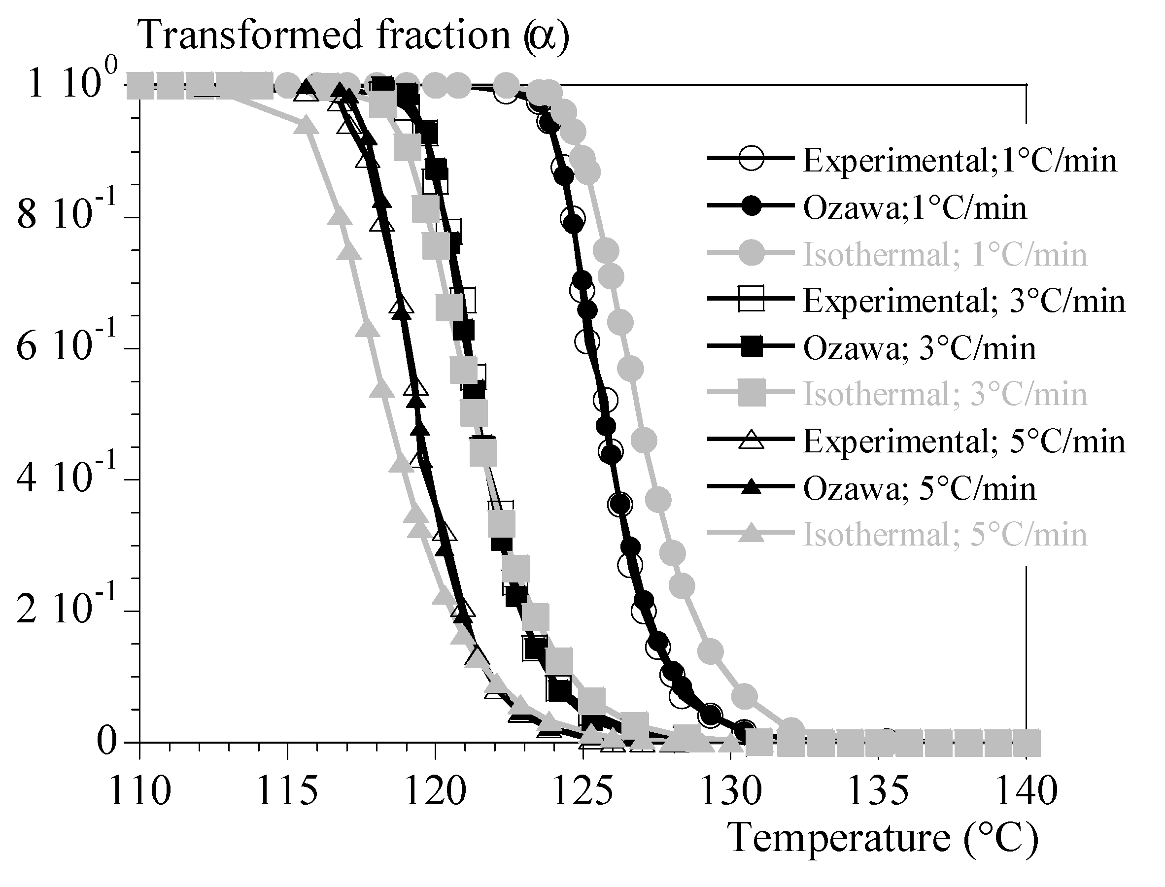
In parallel, the Ozawa’s model (Eq. (10)) was applied to tests performed under constant cooling rates and the function was estimated for a value of n equal to 3 (Eq. (17), following [27].
The respective effectiveness of the two identifications can be compared on Figure A1 in appendix. In the following, first route is referred to as “Avrami’like” approach whereas the second is referred as Ozawa’s model. Let’s conclude that the first one (from isothermal measurements) should allow to estimate orders of magnitude whereas Ozawa’s model is accurate. In our context, these estimations will be used as input data to validate rheological models in realistic conditions (i.e., in conditions where crystallization kinetics cannot be measured in situ).
4.2. Rheology in isothermal conditions
The isothermal evolutions of the transformed volume fraction and the storage and loss moduli, G’ and G’’, are illustrated in Figure 2a and 2b.
A mechanical stiffening was observed contemporaneously with crystallization observed in DSC. However, the events did not appear to be totally simultaneous in all cases. In fact, it appeared that the mechanical response was postponed compared to the thermal ones. As no artifacts could be found, it could be concluded that mechanical measurements were sensitive to crystallization but not totally driven by the transformed volume fraction or crystallinity ratio as they are related.
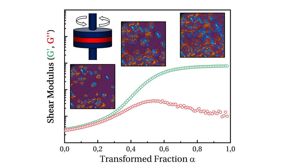
Figure 3 depicts G’ and G’’ vs. α. Depending on temperature, we can notice that mechanical stiffening took place between transformed fraction of 10 % and 45 %. This difference was correlated to the temperature: the lower the temperature the more rapid the stiffening. G’’ exhibited a peak followed by a relaxation upon time. Maximum of the peak appeared for transformed fraction of 20 % at 127.5 °C and 80 % at 135°C. In conclusion, the transformed volume fraction is far to be enough to describe the mechanical state of the material.
In Figure 3, we plot the evolution of Poisson probability. We can notice that crystallization at low temperature is such that mechanical evolution could be observed during the first stage of crystallization: single spherulites and isolated small aggregates. Conversely, crystallization at higher temperature implies a material close to coalescence of spherulites.
As a first approach, storage modulus versus transformed fraction data have been described using General Effective Medium (GEM) law. This analysis aimed to determine a parameter equivalent to a mechanical percolation threshold, specifically the transformed fraction at which a percolating cluster of spherulites appears. This law allows to fit both part of the curve (below and above percolating threshold) at the same time. It was initially used to describe electrical percolation phenomenon [39] but has been recently adapted to describe percolation of spherulites during crystallization processes [40]. The GEM equation is as follows (Eq. (18)):
is the percolation threshold in term of transformed fraction. is the storage modulus in the melting state (i.e., at ). is the storage modulus in solid state (i.e., at ). Exponent describes the slope of the curve below percolation threshold, while exponent describes the slope of the curve above percolation threshold. Using this equation as it stands resulted in satisfactory agreements with experimental data. However, the fit parameters obtained were not physically consistent: e.g., percolation threshold value at 125 °C was estimated at a transformed fraction of 1.1. Therefore, it seemed that this law was not totally adapted to the studied system and therefore, it was chosen to investigate another phenomenological approach.
Before moving forward, let’s notice that, in Figure 3, it is also visible that the trial at 125 °C appeared to be different from the others, whereas it did not reveal any specificity when analysed as a function of time (Figure 2). Indeed, it is well known that isothermal crystallization at low temperatures is always tricky as crystallization can begin during cooling step prior to the test. In our case, crystallization began at higher temperature than 125 °C, during that cooling phase that was not recorded. Let us emphasize that mechanical curves are shifted towards higher temperatures which is a kind of validation.
Finally, Figure 4 depicts N and <R> and illustrates that the different conditions of crystallization did not involve the same number of spherulites or the same maximum average radius.
4.3. Rheology under non-isothermal conditions
Figure 5 and Figure 6 show typical results obtained under non-isothermal conditions (i.e., at constant cooling rates of 0.1 and 5 °C/min, respectively). Figure 5 groups the tests performed at 1 and 5 °C/min by superimposing the evolutions of G’, G’’ and α. It allows to draw the same general conclusions as those obtained under isothermal conditions.
In summary, the mechanical effects of crystallization are contemporaneous with the thermal effects but not completely simultaneous. Stiffness may involve different stages of crystallization depending on the thermal conditions. The higher the crystallization temperature, the more the last stages are involved (high ). Schematically, the crystallizing medium can appear as composed of individual spherulites whose number and radius vary for low crystallization temperatures (high cooling rates) or coalescing spherulites for higher temperatures (low cooling rates). Based on what is known in the field of micromechanics [32,33], this should have a significant impact and make a simple correlation with the crystallinity rate irrelevant. This may also explain the apparent inconsistency of results in the literature regarding this correlation.
Figure 6 superimposes the results of the tests performed under a cooling rate of 0.1 °C/min, which led to a crystallization temperature of 135 °C, and the one performed at constant temperature of 135 °C. To compare isothermal and non-isothermal results, the time scale of isothermal test has been shifted for the drawing. This superposition shows that there is a certain level of similirarity between the two conditions but that the cooling phase before crystallization is important. Simply speaking, the thermal history before crystallization plays a role. In addition, the isothermal conditions allow to observe some relaxation, mainly of G’’, after crystallization which is either hidden or non-existent during controlled cooling.
We can attempt to reformulate these conclusions as follows. The thermodynamics and kinetics of nucleation and growth define the temperature at which the level of crystallinity increases. This temperature controls the contrast in behavior between the two phases. We cannot exclude the possibility that the first stages of crystallization lead to an imperfect ordered phase whose intrinsic properties would evolve with time. At this stage, we do not have any information going in this direction or contradictory.
The fact remains that an attempt at modeling must integrate parameters characteristic of the microstructure and of the contrast of properties. This is why we have defined above the three parameters N, <R>, and .
5. Modelling
5.1. Methodology
The objective of this modelling part is the development of a phenomenological interpolation for G’ and G’’ based on the chosen characteristic parameters. The two moduli were considered independently. Isothermal measurements were first considered to suggest formalisms.
Then, parameters were identified with the solver of EXCEL® software with a mean square type cost function. Identification was possible with all the tests taken one by one. Parameters from isothermal tests exhibited coherent evolution with temperature, except the one at 125 °C that crystallized during cooling step. To better address dependence upon temperature, it was, then, useful to add one non-isothermal test to the database. We chose a test performed at low cooling rate (0.1 °C/min) to stay close to isothermal conditions.
Other experiments under constant cooling rates were used as validation trials. In that step the transformed volume fraction was also numerically estimated from our identified kinetics. The two estimates (from Avrami’s and from Ozawa’s equations) were considered.
5.2. Rheology vs. crystallization
Basic assumptions were that G’ should be controlled by the microstructure and the temperature, whereas G’’, that is related to dissipation, should be controlled by the amount of amorphous phase and by the mobility of the chains inside it. To account for the later assumption, some parameters were assumed to depend on temperature in the same manner as the growth rate, imagining that the same fundamental motions should be involved. This was done by mimicry to isokinetics assumption. For convenience, we assumed we can write those parameters as a function of growth rate of spherulites, . Best fits were obtained with formalisms given in Eq. (19).
in Eq. (19) corresponds to the storage modulus of PP when crystallinity ratio is zero. is the storage modulus when solid (spherulites). Equation expresses the fact that the storage modulus, G’, gradually increases from to when crystallization occurs in a manner that should depend on the number and the radius of the spherulites, the level of impingements between them as well as the temperature (if parameters depend on temperature).
Alternatively, is the loss modulus of the liquid. The one of the solid PP, , should depend on the crystallinity ratio (0.54 in this paper), , the loss modulus of the crystal, , and the loss modulus of the amorphous phase included in the spherulites, . Equation expresses that G’’ results from the combination of dissipation in the crystal, the one in the liquid, and the one in the amorphous phase, with some disturbance effects due to microstructure (term in . These latter are expressed as a function of Evans expectancy to mimic .
and were estimated from rheological measurements and were not identified with other parameters in our calculations. Indeed, the experimental sets were too limited to allow its identification from isothermal trials.
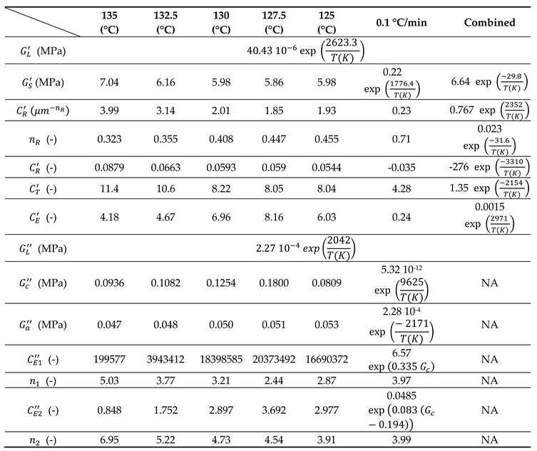
Parameters to identify are then: on one hand (G’) and and on the other hand (G’’). Data resulting from identification from tests, one by one and combined, are gathered in Table 2.
5.3. Rheology vs. melting
Melting results from a progressive disappearance of lamellae, keeping spherulitic superstructure unchanged. So, it was considered that storage and loss modulus during melting results from a mixing law (Eq. (20)).
For simplicity in this paper, we only used data for heating rates of 1 °C/min, i.e.:
6. Results
The equations (19) and the parameters of Table 2 make possible to well reproduce isothermal evolution of G’ and G’’ whatever the protocol (Figure 7). Nevertheless, only identification involving at the 0.1 °C/min could be extrapolated to non-isothermal tests.
Figure 8a displays the experimental (dashed lines) and calculated (symbols) evolutions of the modulus G' as a function of the temperature for cooling rates of 1, 3 and 5 °C/min. These tests were not used when identifying the parameters. This is therefore a validation. Only the formalism of the equation (19) was used. Parameters were identified in two ways:
1-by using only the test at 0.1 °C/min and interpolating the crystallization kinetics with Ozawa's formalism (eq. (10)).
2- by combining the test at 0.1 °C/min and the isothermal tests and interpolating the kinetics of not isothermal crystallization with the formalism of Ozawa (Eq. (10)).
Validations were adapted in 4 ways:
by using the coefficients 1 under the conditions of identification 1 (Ozawa crystallization, hollow squares).
by using the coefficients 1 and interpolating the crystallizations during the validation tests from the isothermal tests (hollow circles).
by using the coefficients 2 under the conditions of identification 2 (Ozawa crystallization, filled squares).
by using the coefficients 2 and interpolating the crystallizations during the validation tests from the isothermal tests (filled circles).
Figure 8b depicts the efficiency of those 4 routes for the test under cooling rate of 0.1 °C/min.
Our approach reproduces the effect of the cooling rate and the order of magnitude of the moduli. However, predictions of the rate effect are clearly better if the identification is done on a larger data set (identification 2). In parallel, it seems that a better estimation of the crystallization kinetics is favorable (Ozawa model). Finally, the model would deserve to be adjusted to better identify the modulus after crystallization. However, to achieve that point it will be necessary to consider the relaxations specific to the amorphous phase. Further study is therefore still needed.
Regarding G'', the proposed formalism was able to independently reproduce the isothermal and the non-isothermal tests, but a unique set of parameters was not found. This difficulty in reproducing the two conditions through a single set of parameters is not surprising. G'' contains the viscoelastic effects and has therefore a particular relation to time. We could however propose a modeling of the cooling rate effect that was quite satisfactory from identification with the test at 0.1 °C/min (Figure 9).
As for the melting tests, they were sufficiently well reproduced with the simple mixing law. It was then possible to reproduce cycle melting – crystallization with a good agreement (Figure 10).
Note, however, that each condition was treated independently, assuming that the initial states were equilibrium: total and relaxed melting and complete crystallization at equilibrium. Cycle modeling will require considering intermediate crystalline states. In the same way, a complete modeling now requires accounting for the relaxations specific to the amorphous phase, in particular the principal relaxation. This will require further work.
Let us conclude here that the feasibility of the approach is validated. It represents a pragmatical and simple alternative to the necessary theoretical developments.
7. Conclusion
The viscoelastic properties of PP during crystallization were studied under isothermal conditions and at constant cooling rates. It was shown that, whatever the conditions, the mechanical effects of crystallization cannot be modelled by considering the degree of crystallinity alone.
In fact, the mechanical effects of crystallization are contemporaneous with the increase in the transformed volume fraction, but not simultaneously.
Stiffening can occur at different stages of crystallization, depending on the thermal conditions. This could be one of the reasons for the discrepancies and controversies in the literature.
In summary, the higher the crystallization temperature, the more coalescence between spherulites is involved when the modulus increases.
Consequently, the crystallizing medium must be composed of individual spherulites at low temperature (high cooling rate), aggregates at medium temperature or coalescing spherulites at high temperature (low cooling rate), for the storage and loss moduli to change significantly.
This represents a real improvement in knowledge in this area.
One reason for this could be that the contrast in the behavior between the two phases is of paramount importance in determining the properties of the crystallizing medium.
This justifies more in-depth studies aiming at combining microstructure modelling and micromechanical modelling of the mechanical behavior of the heterogeneous medium.
In a first approach, we show that one can refer to the microstructure at the spherulite scale in a simplified way to suggest phenomenological models for the storage and loss modules.
This represents a second important result of the study. It has been possible to propose simple mathematical models of the evolution of the two moduli as a function of the temperature for different cooling rates, which requires only classical crystallization analyses, growth rate measurements and rheometric tests to be used.
This could help to estimate residual stresses in additive manufacturing until more rigorous models are developed.
Appendix A
References
- H. Biskas, P. Stavropoulos and G. Chryssolouros, "Additive manufacturing methods and modelling; a critical review," Int J Adv Manuf Technol, vol. 83, p. 389–405, 2016.
- Haudin, J.-M.; Boyer, S.A.E. Crystallization of Polymers in Processing Conditions: An Overview. Int. Polym. Process. 2017, 32, 545–554. [Google Scholar] [CrossRef]
- P. Sreejith, K. Kannan and K. R. Rajagopal, "A thermodynamic framework for the additive manufacturing of crystallizing polymers. part I: A theory that accounts for phase change, shrinkage, warpage and residual stress.," Int. J. Eng. Sci., vol. 183, p. 103789, 2023.
- Boutahar, K.; Carrot, C.; Guillet, J. Crystallization of Polyolefins from Rheological MeasurementsRelation between the Transformed Fraction and the Dynamic Moduli. Macromolecules 1998, 31, 1921–1929. [Google Scholar] [CrossRef]
- N. V. Pogodina and H. H. Winter, "Crystallization as a Physical Gelation Process," Macromolecules, vol. 31, p. 8164, 1998.
- Lamberti, G.; Peters, G.W.M.; Titomanlio, G. Crystallinity and Linear Rheological Properties of Polymers. Int. Polym. Process. 2007, 22, 303–310. [Google Scholar] [CrossRef]
- Han, S.; Wang, K.K. Shrinkage prediction for slowly-crystallizing thermoplastic polymers in injection molding. Int. Polym. Process. 1997, 12, 228–237. [Google Scholar] [CrossRef]
- Pantani, R.; Speranza, V.; Titomanlio, G. Simultaneous morphological and rheological measurements on polypropylene: Effect of crystallinity on viscoelastic parameters. J. Rheol. 2015, 59, 377–390. [Google Scholar] [CrossRef]
- Aris-Brosou, M.; Vincent, M.; Agassant, J.-F.; Billon, N. Viscoelastic rheology in the melting and crystallization domain: Application to polypropylene copolymers. J. Appl. Polym. Sci. 2017, 134. [Google Scholar] [CrossRef]
- Keith, H.D.; Vadimsky, R.G.; Padden, F.J. Crystallization of isotactic polystyrene from solution. J. Polym. Sci. Part A-2: Polym. Phys. 1970, 8, 1687–1696. [Google Scholar] [CrossRef]
- Keith, H.D.; Padden, F.J.; Vadimsky, R.G. Intercrystalline Links: Critical Evaluation. J. Appl. Phys. 1971, 42, 4585–4592. [Google Scholar] [CrossRef]
- Padden, F.J.; Keith, H.D. Mechanism for lamellar branching in isotactic polypropylene. J. Appl. Phys. 1973, 44, 1217–1223. [Google Scholar] [CrossRef]
- Keith, H.; Padden, F. Twisting orientation and the role of transient states in polymer crystallization. Polymer 1984, 25, 28–42. [Google Scholar] [CrossRef]
- J. D. Hoffman and J. J. Weeks, "Melting process and the equilibrium melting temperature of polychlorotriuoroethylene," J. Res. Nat. Bur. Stand. Sect. A Phys. Chem.,, vol. 66A, no. 1, pp. 13-28, 1962.
- Hoffman, J.D.; Miller, R.L. Kinetic of crystallization from the melt and chain folding in polyethylene fractions revisited: theory and experiment. Polymer 1997, 38, 3151–3212. [Google Scholar] [CrossRef]
- Lauritzen, J.I.; Hoffman, J.D. Extension of theory of growth of chain-folded polymer crystals to large undercoolings. J. Appl. Phys. 1973, 44, 4340–4352. [Google Scholar] [CrossRef]
- Piorkowska, E.; Galeski, A.; Haudin, J.-M. Critical assessment of overall crystallization kinetics theories and predictions. Prog. Polym. Sci. 2006, 31, 549–575. [Google Scholar] [CrossRef]
- M. Avrami, "Kinetics of phase change. I. General theory," J Chem Phys, vol. 7, pp. 1103-1112, 1939.
- M. Avrami, "Kinetics of phase change. II. Transformation–time relations for random distribution of nuclei.," J. Chem. Phys., vol. 8, pp. 212-224, 1940.
- M. Avrami, "Kinetics of phase change. III. Granulation, phase change and microstructure," J. Chem. Phys., vol. 9, pp. 177-184, 1941.
- W. A. Johnson and R. F. Mehl, "Reaction kinetics in process of nucleation and growth," Trans AIME, vol. 135, p. 416–458, 1939.
- N. Kolmogoroff, "K statisticheskoi teorii kristallizacii metallov," Izvestiya Akad Nauk SSSR Ser Math, pp. 1355-1359, 1937.
- U. R. Evans, "The laws of expanding circles and spheres in relation to the lateral growth of surface films and the grainsizeof metals," Trans Faraday Soc, vol. 41, pp. 365-375, 1945.
- K. Nakamura, T. Watanabe, K. Katayama and T. Amano, "Some aspects of nonisothermal crystallization of polymers. I. Relationship between crystallization temperature, crystallinity and cooling conditions," J Appl Polym Sci, vol. 16, pp. 1077-1091, 1972.
- K. Nakamura, K. Katayama and Amano T., "Some aspects of nonisothermal crystallization of polymers. II. Consideration of the Isokinetic condition," J Appl Polym Sci, vol. 17, p. 1031–1941, 1973.
- Ozawa, T. Kinetics of non-isothermal crystallization. Polymer 1971, 12, 150–158. [Google Scholar] [CrossRef]
- Billon, N.; Barq, P.; Haudin, J.M. Modelling of the Cooling of Semi-crystalline Polymers during their Processing. Int. Polym. Process. 1991, 6, 348–355. [Google Scholar] [CrossRef]
- J.-M. Haudin and J.-L. Chenot, "Numerical and physical modeling of polymer crystallization—Part I: theoretical and numerical analysis," Int Polym Process 2004;19:267–74., vol. 19, pp. 267-274, 2004.
- W. Schneider, A. Koppl and J. Berger, "Non-Isothermal crystallization of polymers," Int Polym Process., vol. 2, pp. 151-154, 1998.
- Kerner, E.H. The Elastic and Thermo-elastic Properties of Composite Media. Proc. Phys. Soc. Sect. B 1956, 69, 808–813. [Google Scholar] [CrossRef]
- Vandommelen, J.; Parks, D.; Boyce, M.; Brekelmans, W.; Baaijens, F. Micromechanical modeling of the elasto-viscoplastic behavior of semi-crystalline polymers. J. Mech. Phys. Solids 2003, 51, 519–541. [Google Scholar] [CrossRef]
- Bédoui, F.; Diani, J.; Régnier, G.; Seiler, W. Micromechanical modeling of isotropic elastic behavior of semicrystalline polymers. Acta Mater. 2006, 54, 1513–1523. [Google Scholar] [CrossRef]
- Luo, Y.-M.; Detrez, F.; Chevalier, L.; Lu, X.; Roland, S. Multiscale framework for estimation of elastic properties of Poly ethylene terephthalate from the crystallization temperature. Mech. Mater. 2023, 181. [Google Scholar] [CrossRef]
- Monasse, B.; Haudin, J.M. Thermal dependence of nucleation and growth rate in polypropylene by non isothermal calorimetry. Colloid Polym. Sci. 1986, 264, 117–122. [Google Scholar] [CrossRef]
- Billon, N.; Haudin, J.M. Determination of nucleation rate in polymers using isothermal crystallization experiments and computer simulation. Colloid Polym. Sci. 1993, 271, 343–356. [Google Scholar] [CrossRef]
- N. Billon, V. Henaff and J.-M. Haudin, "Transcrystallinity effects in high-density polyethylene. II. determination of kinetics parameters," J. Appl. Polym. Sci., vol. 86, no. 3, pp. 734-742, 2002.
- Hoffman, J.D. Regime III crystallization in melt-crystallized polymers: The variable cluster model of chain folding. Polymer 1983, 24, 3–26. [Google Scholar] [CrossRef]
- J. D. Hoffman, L. J. Frolen, G. S. Ross and J. I. Lauritzen Jr., "On the growth rate of spherulites and axiaites from the melt in polyethylene fractions: Regime I and regime II crystallization," J. Res. Natl. Bur. Stand. Sect. A Phys. Chem., vol. 79A, no. 6, p. 671, 1975.
- McLachlan, D.S. An equation for the conductivity of binary mixtures with anisotropic grain structures. J. Phys. C: Solid State Phys. 1987, 20, 865–877. [Google Scholar] [CrossRef]
- D. Roy, D. Audus and K. Migler, "Rheology of crystallizing polymers: The role of spherulitic superstructures, gap height, and nucleation densities. Journal of Rheology," J. of Rheology, vol. 63, p. 851–862, 2019.
Figure 1.
Comparison of transformed volume fraction, , and . a) Schematic definition; b) Probability vs. mathematical expectancy, E.
Figure 1.
Comparison of transformed volume fraction, , and . a) Schematic definition; b) Probability vs. mathematical expectancy, E.
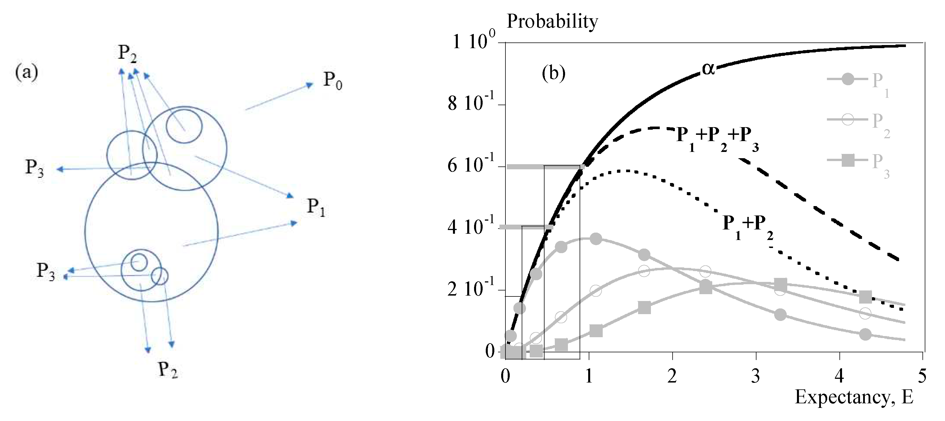
Figure 2.
Isothermal crystallization: comparison between 125, 127.5, 130, 132.5 and 135 °C. a) Transformed volume fraction vs. time. b) Storage module, G’, and loss modulus, G’’ vs. time.
Figure 2.
Isothermal crystallization: comparison between 125, 127.5, 130, 132.5 and 135 °C. a) Transformed volume fraction vs. time. b) Storage module, G’, and loss modulus, G’’ vs. time.
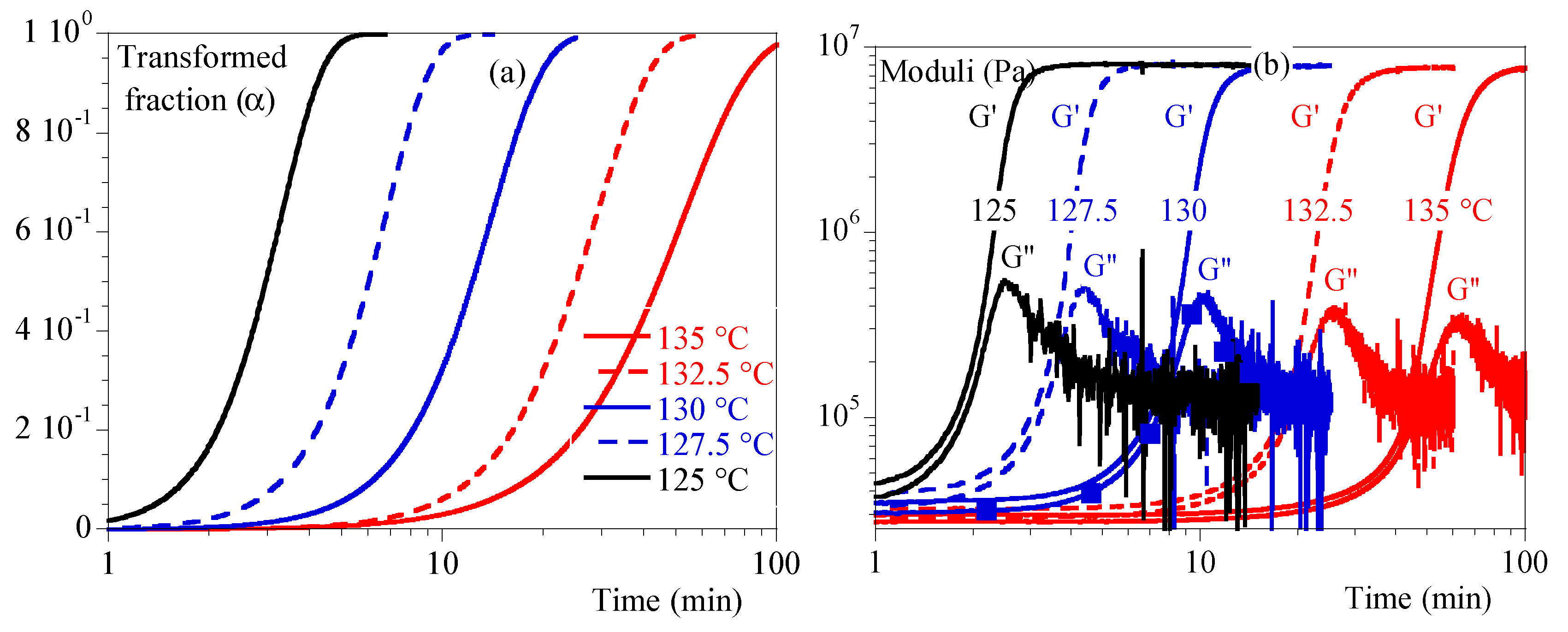
Figure 3.
Isothermal crystallization: comparison between 125, 127.5, 130, 132.5 and 135 °C. a) Storage modulus vs. transformed fraction. B) Loss modulus vs. transformed fraction. Straight line represents transformed fraction. Dashed grey line is (Eq. (2)).
Figure 3.
Isothermal crystallization: comparison between 125, 127.5, 130, 132.5 and 135 °C. a) Storage modulus vs. transformed fraction. B) Loss modulus vs. transformed fraction. Straight line represents transformed fraction. Dashed grey line is (Eq. (2)).
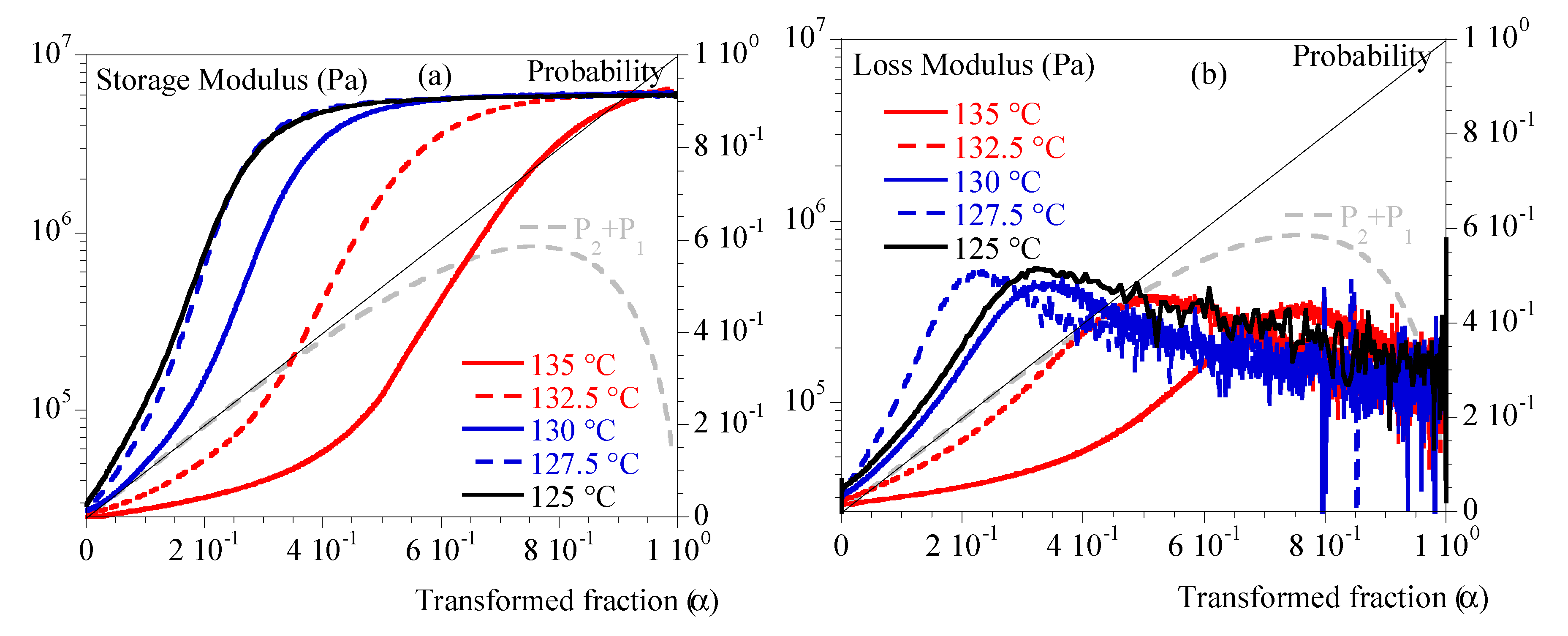
Figure 4.
Isothermal crystallization: comparison between 125, 127.5, 130, 132.5 and 135 °C. a) N (Eq. (12)) vs. transformed fraction. B) <R> (Eq. (15)) vs. transformed fraction. Straight line represents transformed fraction. Dashed grey line is (Eq. (2)).
Figure 4.
Isothermal crystallization: comparison between 125, 127.5, 130, 132.5 and 135 °C. a) N (Eq. (12)) vs. transformed fraction. B) <R> (Eq. (15)) vs. transformed fraction. Straight line represents transformed fraction. Dashed grey line is (Eq. (2)).
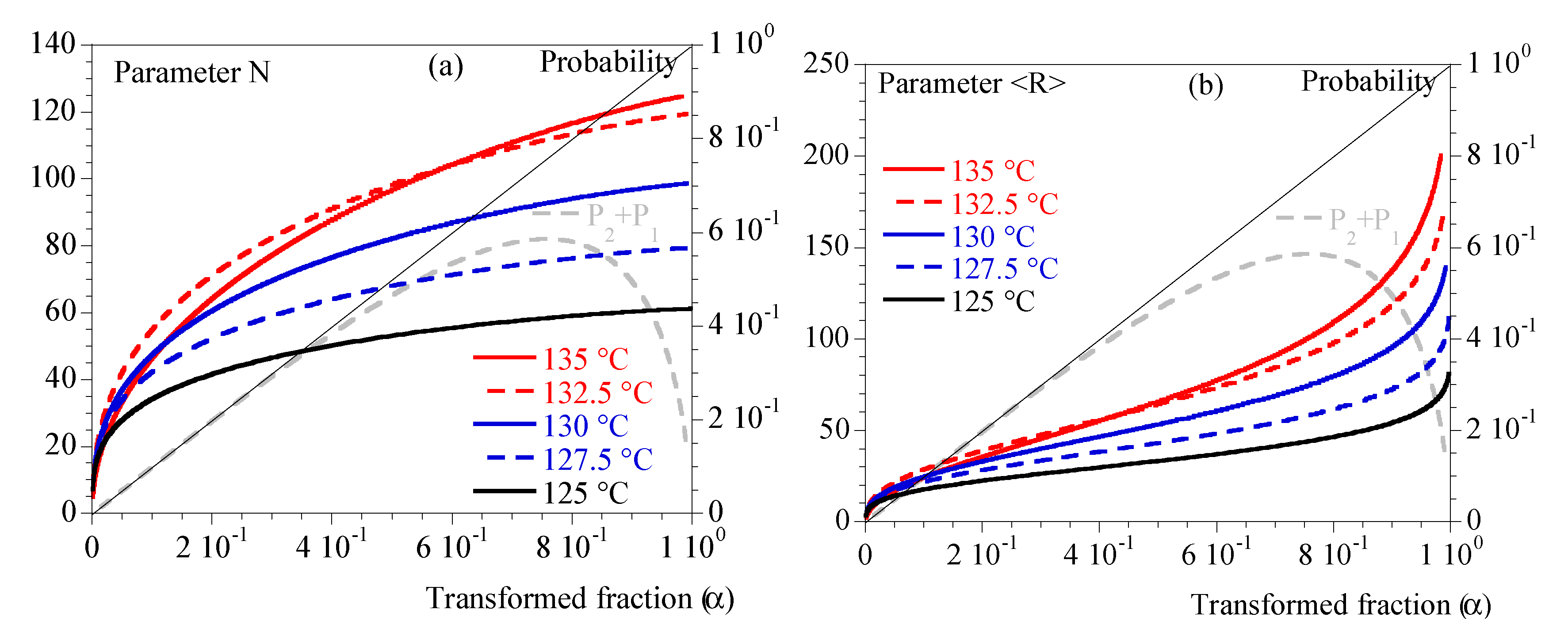
Figure 5.
Mechanical properties during crystallization performed under constant cooling rates. Comparison between 1 (blue) and 5 °C/min (red). Storage modulus, G’, is represented with dashed lines, loss modulus, G’’, with plain lines. Symbols represent (hollow symbols) and (plain symbols).
Figure 5.
Mechanical properties during crystallization performed under constant cooling rates. Comparison between 1 (blue) and 5 °C/min (red). Storage modulus, G’, is represented with dashed lines, loss modulus, G’’, with plain lines. Symbols represent (hollow symbols) and (plain symbols).
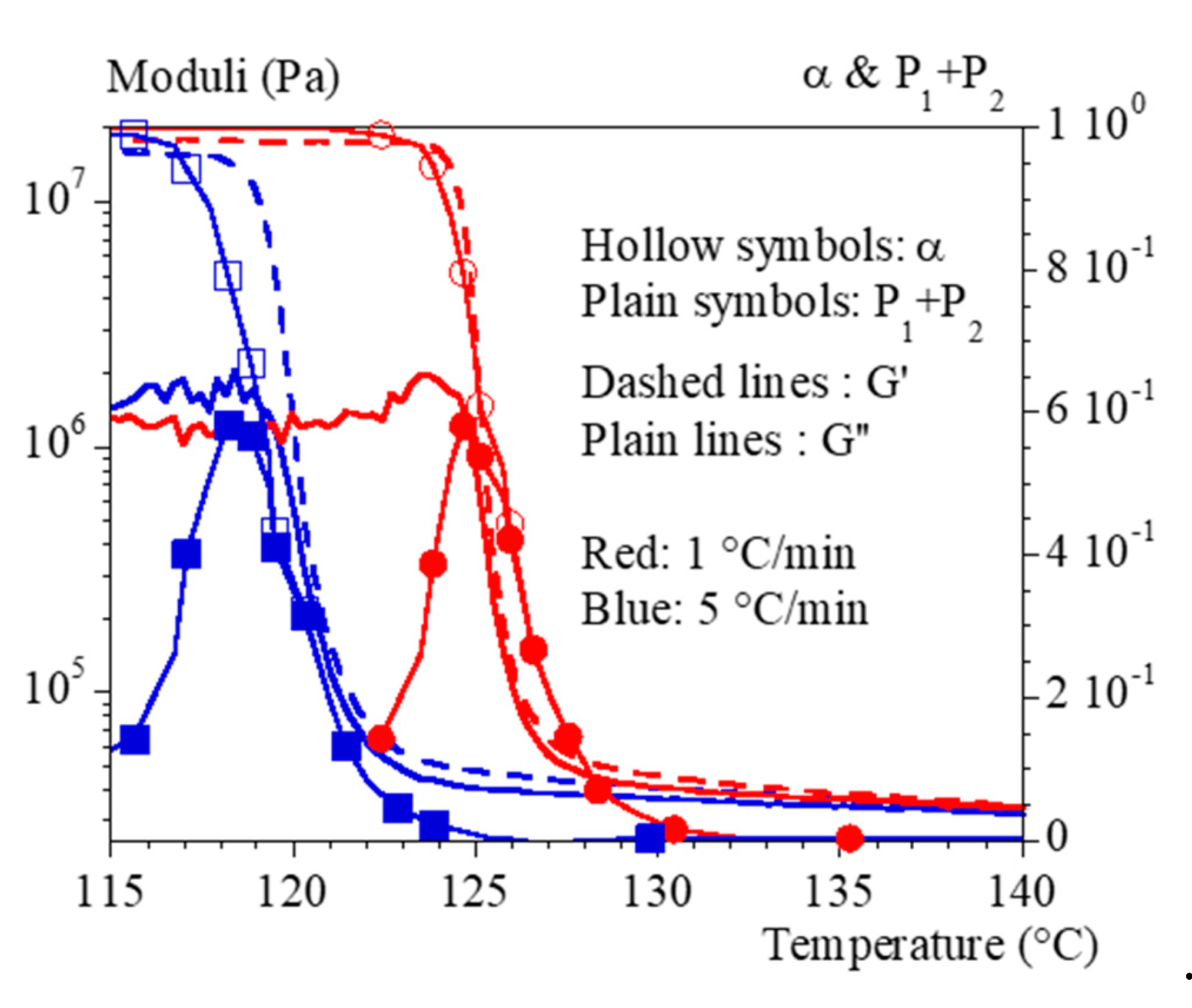
Figure 6.
Mechanical properties during crystallization performed under constant cooling rates at 0.1 °C/min (grey) compared to isothermal crystallization at 135 °C (black). Storage modulus, G’ is represented with dashed lines, loss modulus, G’’, with plain lines. Symbols represent .
Figure 6.
Mechanical properties during crystallization performed under constant cooling rates at 0.1 °C/min (grey) compared to isothermal crystallization at 135 °C (black). Storage modulus, G’ is represented with dashed lines, loss modulus, G’’, with plain lines. Symbols represent .
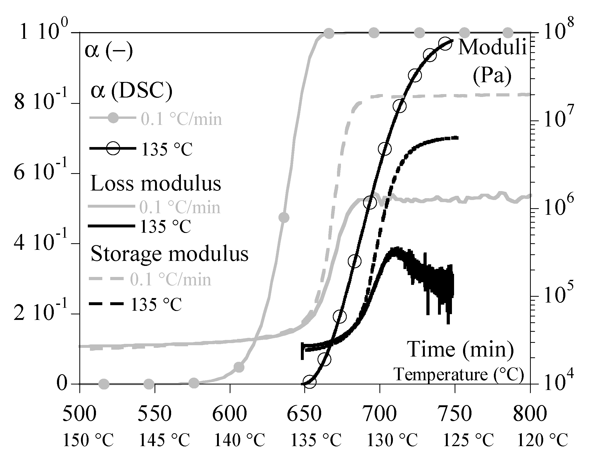
Figure 7.
Storage and loss moduli (G’ and G’’, resp.) vs. time during isothermal crystallization. Comparison between experiments (dashed and plain lines, resp.) and calculus. Calculus 1 is based on identification one by one. Calculus 2 combines isothermal tests and tests under 0.1 °C/min.
Figure 7.
Storage and loss moduli (G’ and G’’, resp.) vs. time during isothermal crystallization. Comparison between experiments (dashed and plain lines, resp.) and calculus. Calculus 1 is based on identification one by one. Calculus 2 combines isothermal tests and tests under 0.1 °C/min.
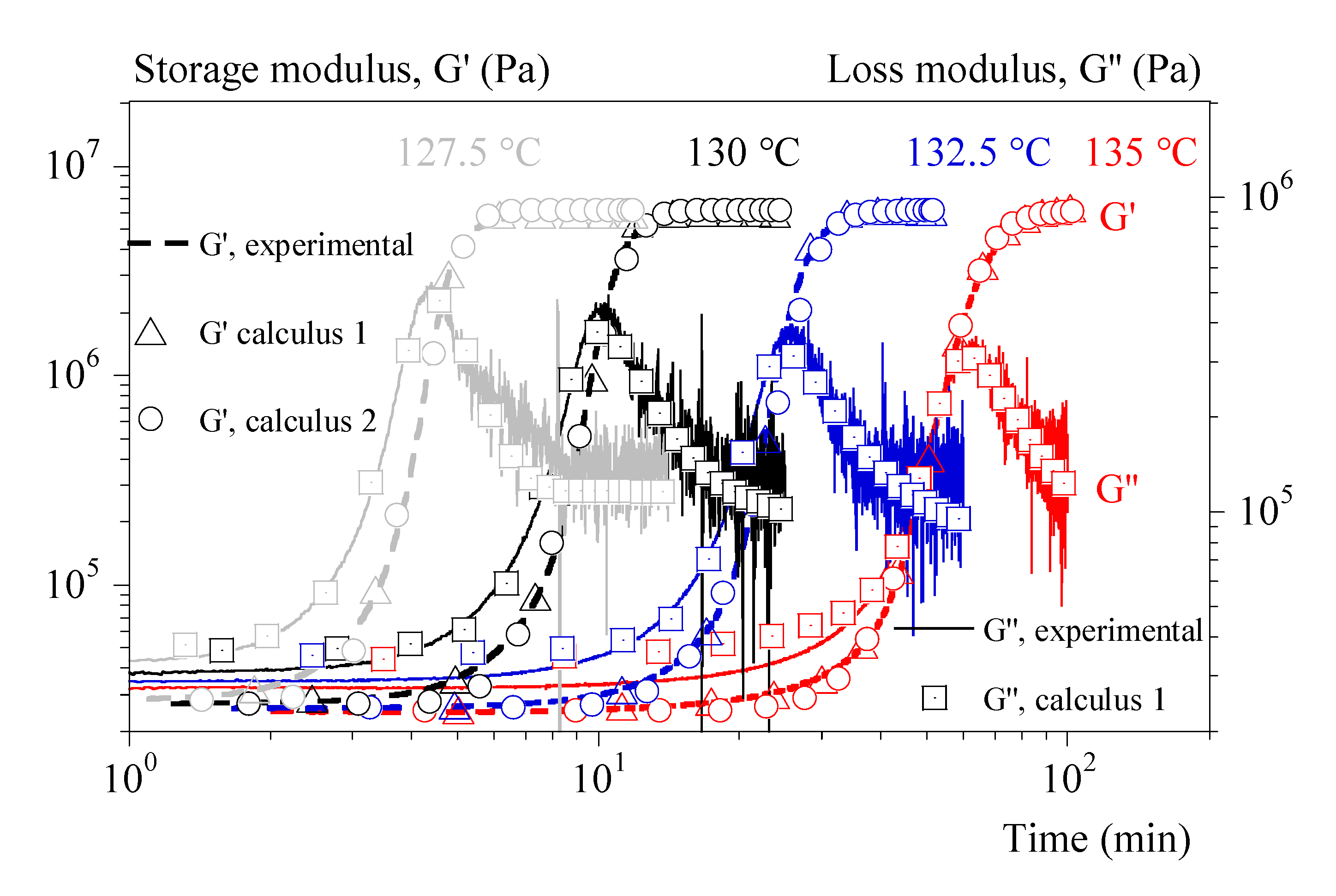
Figure 8.
Validation of equation (18) for storage modulus, G’. a) Comparison between experiments (dashed lines) and calculus (symbols). Colors refer to cooling rates; hollow squares: identification with tests at 0.1 °C/ and Ozawa crystallization; hollow circles: identification with tests at 0.1 °C/ and Avrami like crystallization; filled squares: combined with isothermal tests identification and Ozawa crystallization; filled circles: combined with isothermal tests identification and Avrami like crystallization. b) Results of a cooling rate of 0.1 °C/min.
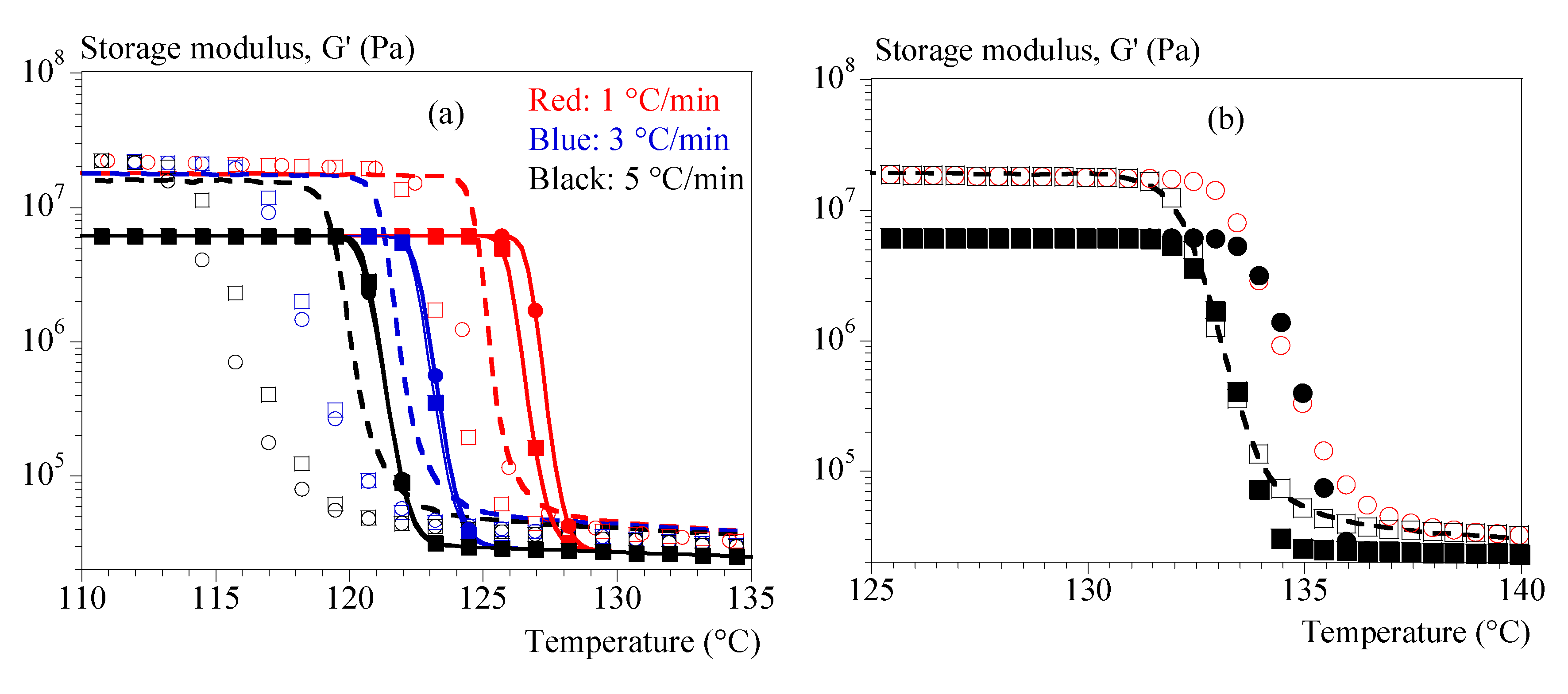
Figure 9.
Validation of equation (18) for loss modulus, G’’. Comparison between experiments (dashed lines) and calculus (symbols). Colors refer to cooling rates; hollow squares: identification with tests at 0.1 °C/ and Ozawa crystallization.
Figure 9.
Validation of equation (18) for loss modulus, G’’. Comparison between experiments (dashed lines) and calculus (symbols). Colors refer to cooling rates; hollow squares: identification with tests at 0.1 °C/ and Ozawa crystallization.
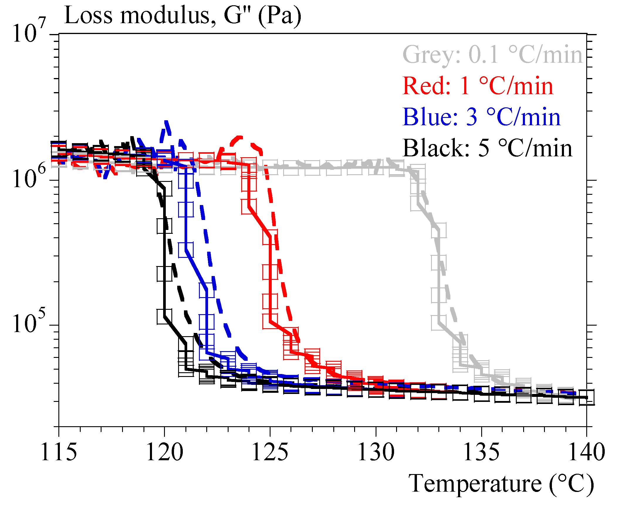
Figure 10.
Cycle heating – cooling at 1 °C/min; Comparison experiments – calculation.
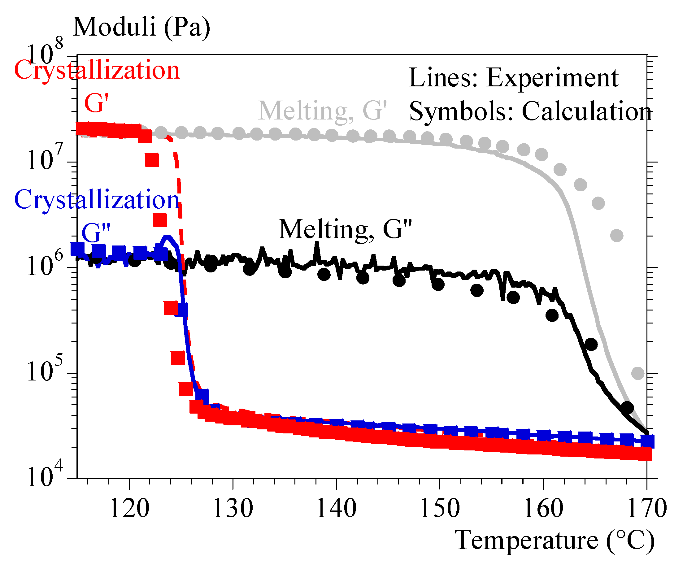

Table 1.
Isothermal characteristics for crystallization. Parameters are defined in Eqs. (10) and (11).
Table 1.
Isothermal characteristics for crystallization. Parameters are defined in Eqs. (10) and (11).
| Temperature(°C) | 125 | 127.5 | 130 | 132.5 | 135 |
|---|---|---|---|---|---|
|
(µm/min) |
20.8 | 13.2 | 7.93 | 4.68 | 2.69 |
|
(min-n) |
1.77 x 10⁻² | 2.46 x 10⁻³ | 7.08 x 10⁻⁴ | 1.59 x 10⁻⁴ | 2.52 10-4 |
| N | 3.39 | 3.15 | 2.75 | 2.60 | 2.09 |
|
for n=3 (min-3) |
4.00 x 10⁻⁵ | 8.33 x 10⁻⁵ | 9.12 x 10⁻⁴ | 4.51 x 10⁻³ | 2.81 x 10⁻² |
|
(µm-3.min3) |
3.13 x 10⁻⁶ | 2.00 x 10⁻⁶ | 1.78 x 10⁻⁶ | 7.96 x 10⁻⁷ | 2.10 x 10⁻⁶ |
Table 2.
Parameters of equation (18) to express G’ and G’’ as a function of T.
Disclaimer/Publisher’s Note: The statements, opinions and data contained in all publications are solely those of the individual author(s) and contributor(s) and not of MDPI and/or the editor(s). MDPI and/or the editor(s) disclaim responsibility for any injury to people or property resulting from any ideas, methods, instructions or products referred to in the content. |
© 2023 by the authors. Licensee MDPI, Basel, Switzerland. This article is an open access article distributed under the terms and conditions of the Creative Commons Attribution (CC BY) license (http://creativecommons.org/licenses/by/4.0/).
Copyright: This open access article is published under a Creative Commons CC BY 4.0 license, which permit the free download, distribution, and reuse, provided that the author and preprint are cited in any reuse.


