1. Introduction
The radar sensor measurements may either be a clutter or a target measurement, so that target existence and trajectory are not a priori known. Target measurements are only present in a scan with some probability of detection
PD < 1 [
1]. In a multi-target situation, the measurements may have also originated from one of various targets, but the number and distribution of targets in the surveillance area is unknown. Automatic tracking in this environment initiates tracks using both target and clutter measurements. If a track follows a target, we call it a true track; otherwise we call it a false track [
2]. To confirm likely tracks and terminate unlikely ones, a track quality measure is necessary. Some standard track quality measures include the probability of the tracks are initialized using measurements, thus both true tracks and false tracks simultaneously exist [
3].In many radar applications, the user has knowledge of the density and distribution of clutter and probability of detection, based on the known parameters, wants to select an optimal algorithm to achieve effective target tracking
The multiple hypotheses tracking (MHT) [
3] is one of the first algorithms which solve multiple measurement-to-track association hypotheses for target tracking in clutter. The measurement-oriented MHT, often known as the Reid algorithm [
4] forms new tracks and measurement allocation hypotheses centered on global origin of measurements. The MHT uses statistical methods to discriminate between false and true tracks. The probability of target existence obtained by utilizing Markov chain propagation models and Bayes update is used as the track quality measure in Integrated Probabilistic Data Association (IPDA) of [
5] and Integrated Track Splitting (ITS). Track estimates obtained from IPDA are conditional on target existence; they depend only on selected measurements and not on the probability of target existence, which is also the case with ITS.
The single target Integrated Track Splitting (ITS) [
6] and Multi-target Joint ITS (JITS) and Linear Multi-target ITS (LMITS) [
7] are generalizations of IPDA, JIPDA and LMIPDA respectively [
8]. They more precisely approximate the trajectory state by a Gaussian Mixture. The MHT, IPDA and ITS based algorithms are derived assuming linear trajectory propagation and linear measurement model. Some nonlinearity may be accommodated by measurement conversion [
9] and by replacing the Kalman filter (KF) with the Extended KF (EKF)[
10,
11] or the Unscented KF (UKF) [
12,
13] within IPDA and ITS.
Nonlinear measurements, e.g. Bearings Only Tracking (BOT), Time Difference of Arrival (TDOA), have measurement likelihoods which are not Gaussian. Any distribution may be approximated by a Gaussian Mixture [
14]. This is used by the Gaussian Mixture Measurement likelihood approximation ITS (GMM-ITS) [
15], which approximates both the measurement likelihoods and the posterior trajectory state PDF by Gaussian Mixtures. The GMM-ITS may be used in more difficult situations where the EKF and UKF do not deliver adequate performance [
16]. SMC methods are powerful tools in Bayesian filtering and have been applied to multi-target problems [
17]. However, no principled SMC implementations have been proposed in the context of FISST.
The multi-target posterior is represented by a large set of weighted random samples (particles), possibly of different dimensions, and is propagated over time using the importance sampling and re-sampling strategy of the standard particle filter. The direct approach of standard SMC methods to propagate the intensity function would fail because the intensity function is not a probability density function and the PHD recursion is not a standard Bayes recursion.
The particle filters [
18] sample nonlinear (non-Gaussian) state PDF by a set of random particles. The particle filters have been successfully applied to a wide range of estimation problems. On the negative side, a large number of particles are often needed for difficult multidimensional scenarios, which typically results in about one to two orders of magnitude higher computational requirements compared to ITS [
19].
However, the publications concentrate on trajectory estimates, without the track quality measure and false track discrimination (FTD). The particle filters for target tracking in clutter have been proposed in [
20]. Some of algorithms use compensation of non-linearity [
21] or augmented hybrid particles that consist of both the base state and the modal state to realize interacting multiple model (IMM)[
22]. These publications concentrate on trajectory estimates only, without calculating a track quality measure and applying it for the FTD. Furthermore, they all assume a known and uniform clutter measurement density, which rarely occurs in real applications. Each track trajectory PDF is represented by a disjoint set of components. The probability of target existence is integrated into the track state. The FTD may use the probability of target existence as the track quality measure. The data association is included to stochastically discriminate against clutter measurements, and the probability of target existence is recursively calculated for use in the false track discrimination. In this paper, we examine the effectiveness of the well-known ITS algorithm in complex motion scenarios, in order to evaluate its applicability in an environment of variable clutter density [
23].
Rest of the paper is organized as follows. The problem statement and models is presented in Section II. Section III derives the SMC probability data association filter (SMC PHD) followed by the results of simulations, presented from Section IV. Concluding remarks will be given in Section V
2. Problem Statements
Consider dynamic state estimation problem, in which the state varies with time. Preamble involves determining the existence and the trajectory of possible targets in the surveillance space, by comparing random measurements received by the sensor with the applicable stochastic models. We use superscripts τ to denote tracks, and also targets followed by tracks.
-
A.
Targets model
We use the Markov Chain One model [
24] for the propagation of the probability of target existence Ψ
k. This model assumes that a target may exist and when it does it is always detectable with a given probability of detection
PD, or it may not exist [
25]. During the targets maneuvering, the motion can be changed at random times. The dynamic models for target τ, target state
, at time k, denotes by:
where
is the propagation matrix,
denotes dynamic model and the
process noise with a zero mean white Gaussian sequence with known covariance matrix
. In the following, the superscript τ refers to the track variables, while the same variables without the superscript refer to the general case. At each scan
k, the sensor returns a random number of the random target and clutter measurements. The measurement of the existing and detectable target is taken with a probability of detection [
26].
-
B.
Measurements models
Measurements may originate from the targets as well as from other objects. The clutter measurements follow the Poisson distribution. We assume that the uniform intensity of the Poisson process at point y in the measurement space, termed here the clutter measurement density and denote by
ρ(y) is a priori known, or can be estimated using the sensor measurements. At time k, one sensor delivers a set of measurements denoted by
. Denote by
the sequence of selected measurement sets up to including time interval
k,
. The measurements model of target τ, is given by the [
27]:
where
are known measurements matrix,
is measurements noise, usually assumed to zero mean white and uncorrelated Gaussian noise sequence with known measurements covariance matrix
[
28].
-
C.
Clutter model
At each scan the sensor returns a random number of clutter measurements, which is modeled by the non-homogeneous Poisson process with known clutter measurements density
(
i -is the index of measurements). The number of clutter point
in all regions of the measurements space are independent. Tracks may be initiated using clutter measurements, and they may be initiated with target measurements but after some time start following clutter measurements. In both situations, there is no target associated with tracks. In that manner, the target existence being (followed by each initialized track) is a random event [
29].
3. Integrated Track Splitting Approach
In ITS, each track is treat as union of components. The track state estimate of each component is the output of a filter which is given a single measurement at each scan. Thus each component represents a possible track-to-measurement association history. All components are mutually exclusive and consists the probability of the component existence and the component state estimate probability density function (PDF), conditioned on the component existence [
30].
In general, ITS consist four iterative steps. Those are:
- a)
Prediction step, where is calculated predicted state for each component, from previous time interval, probability that component is correct and probability of target existence.
- b)
Measurements selection where is calculated the likelihoods of each measurements and each component, provides set of new measurements.
- c)
Data association step provides a posteriori of target existence, a posteriori probability that measurement i is the detection of track τ, at the time interval k, denotes by .
- d)
Track update step provides updated target trajectory state estimate, for each track τ.
Consider the track state at time k by the discrete variable . Let’s defined discrete event where following cases is possible for tracking target:
- case where target τ exist and following target,
-
- case where target τ does not exist.
Also, the case that measurements are (or none) the target detection, can have two outcomes:
, the event that none of the validated measurements is a target τ detection, at the time interval k
, the event that measurements i is a target τ detection, at the time interval k.
3.1 Prediction Step
At the beginning of the prediction step, we associate each track by the probability of existence [
31] from time interval
k-:
Consider track state estimate PDF by the
On the same time, we define set of track components, denominate by
c, with probability
, by the equations:
and its associated components state PDF, by the following equation:
where P(.) denotes total probability. We assume that the track trajectory propagation PDF is Gaussian function [
32]:
Track state PDF is Gaussian mixture:
where component probability prediction is given by the:
and
Ck is total number of components, at the time interval
k.
Consider the Markov Chain One model, for the propagation of the probability of target existence. That’s, if the target exists, its measurement will also be present with the probability of detection
. In general, the propagation of the probability of target existence
from time
k − 1 to time
k is given by:
The value of
is typically assumed constant, while
. Value of
depends on the time interval between measurements. The track trajectory state estimate PDF is a set of track components in the manner of ITS, where each track component corresponds to a unique measurement history. Sufficient statistics for each track component are the probability of track component existence, and the track component state estimate PDF, both conditional on target existence. The track component state estimate PDF depends on the estimator applied for each track component. In this paper a KF state estimator for each track component is performed, thus the state estimate PDF of a track component is a single Gaussian PDF. The track component existence state implies that the measurement history used for the estimate contains the target position at each measurement, given that the target exists. The ‘’null’’ measurement is also used to imply that no selected measurement in that scan is a detection of the (possible) target being tracked. The a posteriori PDF of target trajectory state estimate at time
k − 1 is given by:
where
c denotes the track component, and
denotes the probability that measurement history of track component c is correct, given target existence, and given measurement set Zk−1. Then, track component PDF is given by the Gaussian function:
where is the sum of all component weights is:
Each track component PDF is defined by the mean value
and covariance matrix
of target trajectory estimate, given that the track component measurement history
c is correct, and given that the target exists. When measurement
k arrives, each track component PDF propagates from time
k − 1 to time
k, using the standard KF prediction:
Thus, each track component (mean and covariance) propagates from time
k − 1 to time
k, by the following:
respectively.
3.2 Measurements Selection Step
In this step, each component generates a priori target measurements PDF. The PDF of the target state estimate is the mixture of mutually exclusive component state estimate PDF. The component state estimate PDF is conditioned on the target existence and component data association history being the correct one and the track state estimate PDF is conditioned on the target existence.
Given the assumption of a linear system, this is KF innovations. This PDF can be used to select possible target measurements. If a component does not select a measurement, it is assumed that the corresponding measurement likelihoods are zero. Next, we select component within validation region (gate)
g, by the statistical distance, defined as:
where, measurement prediction
is calculated by the:
and
coavriance of all component is obained by:
A posteriori track state PDF is defined as Gaussian mixture of probability of component and component state PDF by the:
Where track component PDF is given by:
Here, is probability that the probability the target measurement is selected, assuming the target exists and is detected within validation gate.
3.3 Data Association Step
At begining of this step, a poteriori probability of target existence is calculated, by the:
where measurement likelihood ratio at time k is given by the following equation:
Each measurement outcome
is paired with each old track component
c to create a new track component. The likelihood, or a priori PDF of measurement z
k,i under the no measurement merging assumption, is given by:
where measurements prediction is given by the:
and measurements covariance matrix:
3.4 Update Step
At this step, each track update (by the KF update) is performed. Consider ‘’null’’ measurements as the of non-target measurement clutter density in the k
th scan and measurements (as the target measurement clutter density) in the k
th scan. For ‘’null’’ measurements, we have ‘’null’’ component state and covariance, by the following:
and covariance, by the following:
KF reinforcement is given by the:
Component
c state and covariance (for the
ith measuremets) is given by the KF update:
The new component probability is given by the equation:
Finally, (for output purpose only) the track τ state estimate and covariance is given by the following equations:
4. Results of Simulations
The application selected for the study was a two-dimensional (positions and velocities), four-state radar surveillance problem in which the sensor observes both position coordinates. The area under surveillance was
x = [0; 1000] long and
y = [0;1000] wide. Both dimensions were assumed independent. The transition probability for the Markov Chain One model are chosen by ∆
11=0.98. Time interval of scanning is T = 1s. All experiments were conducted on the basis of multi target tracking (MTT) for two targets scenario. Transition and process noise matrix are given by:
Measurements matrix and measurements noise covariance respectively, governed by the matrix:
where
. All experiments were conducted over two types of two-dimensional scenarios. The total duration of both scenarios is 60 scans, repeating over 250 Monte Carlo simulations. All experiments are performed via MATLAB 2015b software. Computer is operate by Intel Core i5=4460 @3.20 GHz processor, with 8MB DDRAM 4 memory. In the experiments, all tracks are initiated with probability of initializing (
probInit). Results are given by the Table1. When the track quality measure rises above a confirmation threshold, the track is confirmed (
probConf) and when the track quality measure falls below the termination threshold, the track is terminated (
probInit/3). The thresholds are determined experimentally to deliver approximately equal numbers of confirmed false track statistics. With the confirmed false tracks statistics approximately equal across all tracks, the success rate of confirmed true tracks allows us to compare false track discrimination performance. Before the start of the simulations, it is necessary to set the same level confirmed false track. This is done by simulating the algorithm without the presence of the targets, for a 250 MC runs. The following definitions of true and false tracks are used:
1) Each initiated track is false with respect to all existing targets.
2) A false track becomes a true track with respect to a target when the state estimate is sufficiently close to the true target state.
3) A track that is true with respect to a target remains true for as long as it selects the target detections.
All results are provided via a plot of the confirmed true tracks,(CTT) diagrams, the overall root mean square error (RMSE) of position, tracking parameters table and normalized tracking efficiency versus probability of detection parametric diagrams. The parameters (per experiment) abbreviated as:
- -
faTrSum, sum of false true tracks,
- -
coFaID, number of confirmed false tracks,
- -
conTrPeak, total number of confirmed true tracks,
- -
CPU time, processor time (for one iteration of algorithm).
For all algorithms, a confirmed false track is present in approximately (average) 20 scans out of total 250 x 60 = 15 000 scans in each simulation experiment. False tracks may be initiated using target measurements, either in conjunction with a clutter measurement, or by using measurements from different targets in different scans. Also, tracks becomes true, when cross the threshold and no longer true, when is greater than known threshold.
4.1. Results of Experiments (Scenario 1)
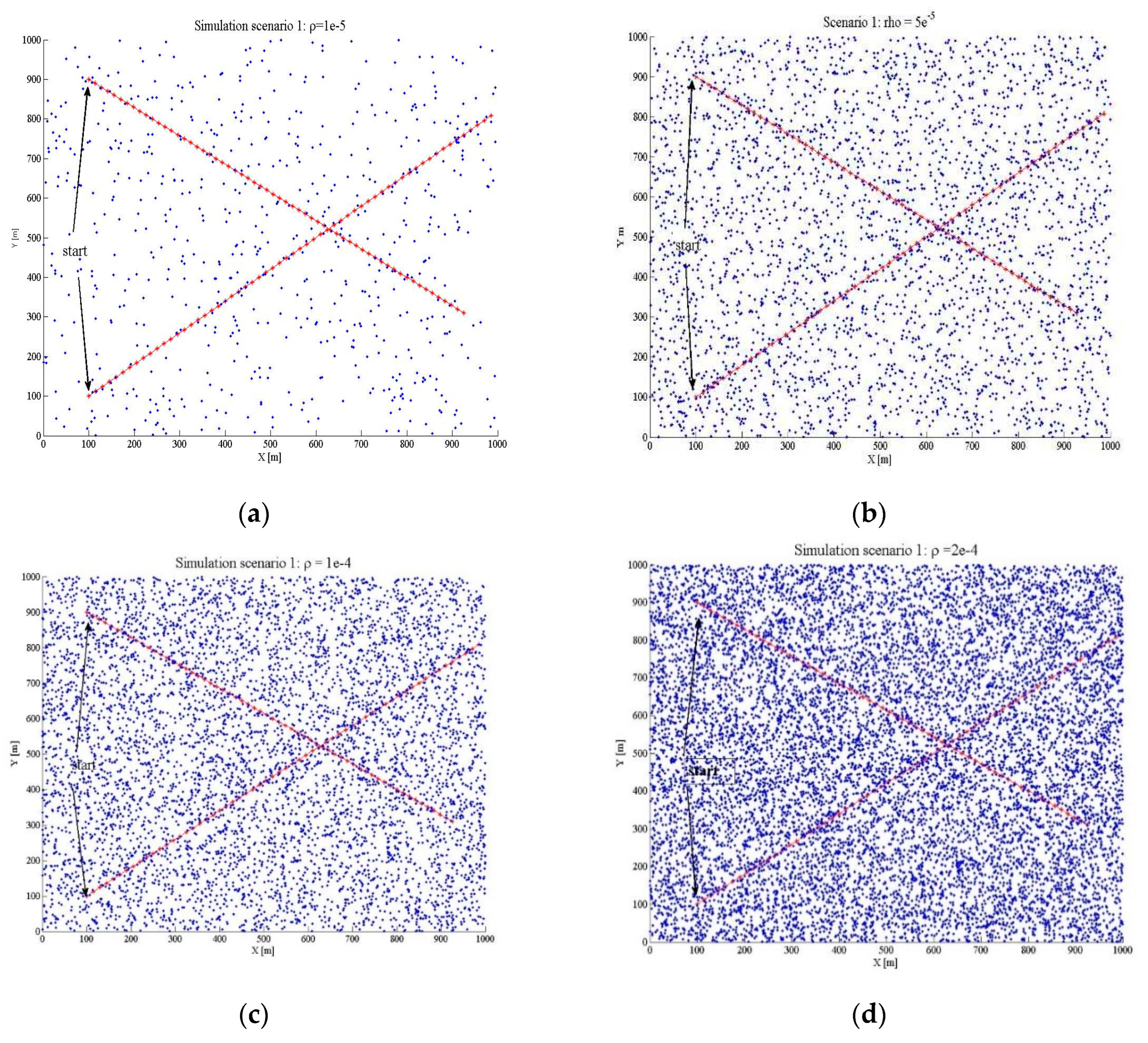
In the scenario 1, two targets move in a straight line at a constant speed. In the second part of the scenario (in about 37 scan), the targets intersect and continue to move in a straight line until the end of the experiment.
Figure 1.
Simulation scenarios 1: a) clutter density , b) clutter density ,c) clutter density , d) clutter density .
Figure 1.
Simulation scenarios 1: a) clutter density , b) clutter density ,c) clutter density , d) clutter density .
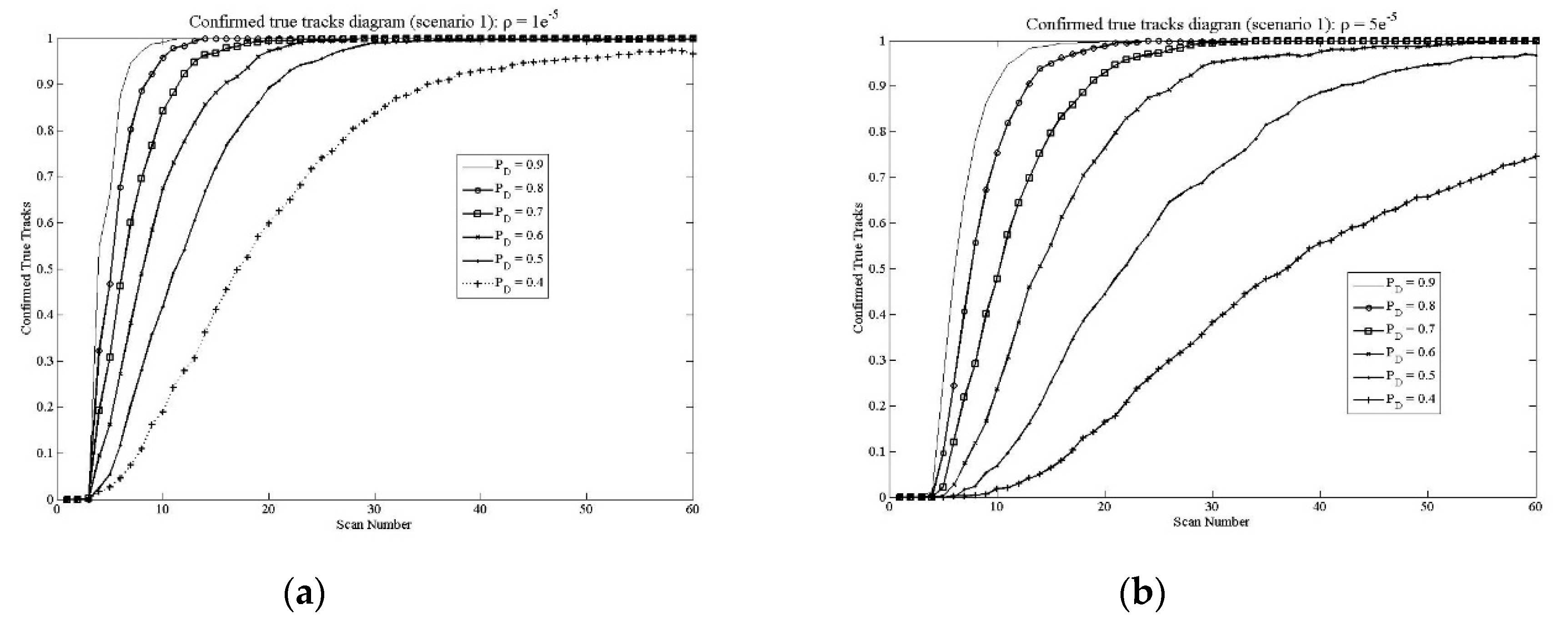
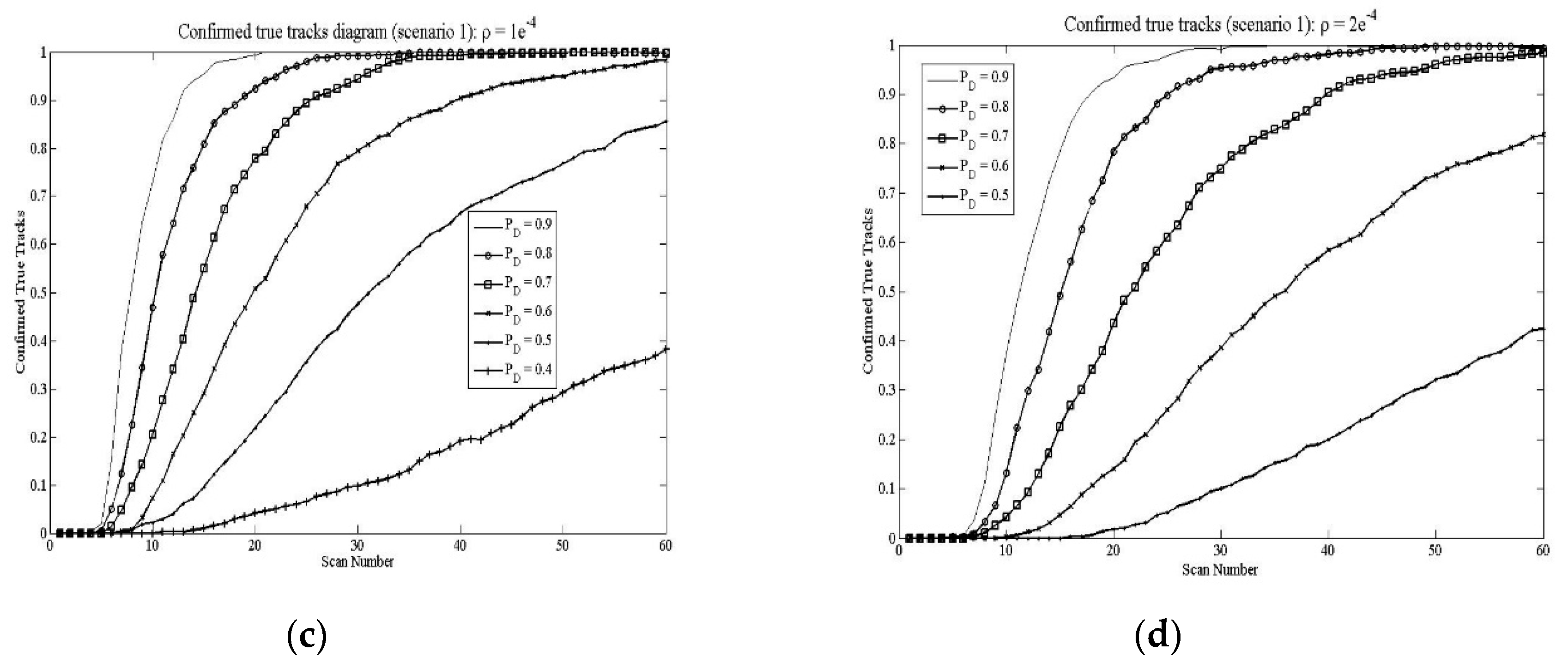
Figure 2.
Confirmed true tracks diagram (scenario 1): a) clutter density , b) clutter density ,c) clutter density , d) clutter density .
Figure 2.
Confirmed true tracks diagram (scenario 1): a) clutter density , b) clutter density ,c) clutter density , d) clutter density .
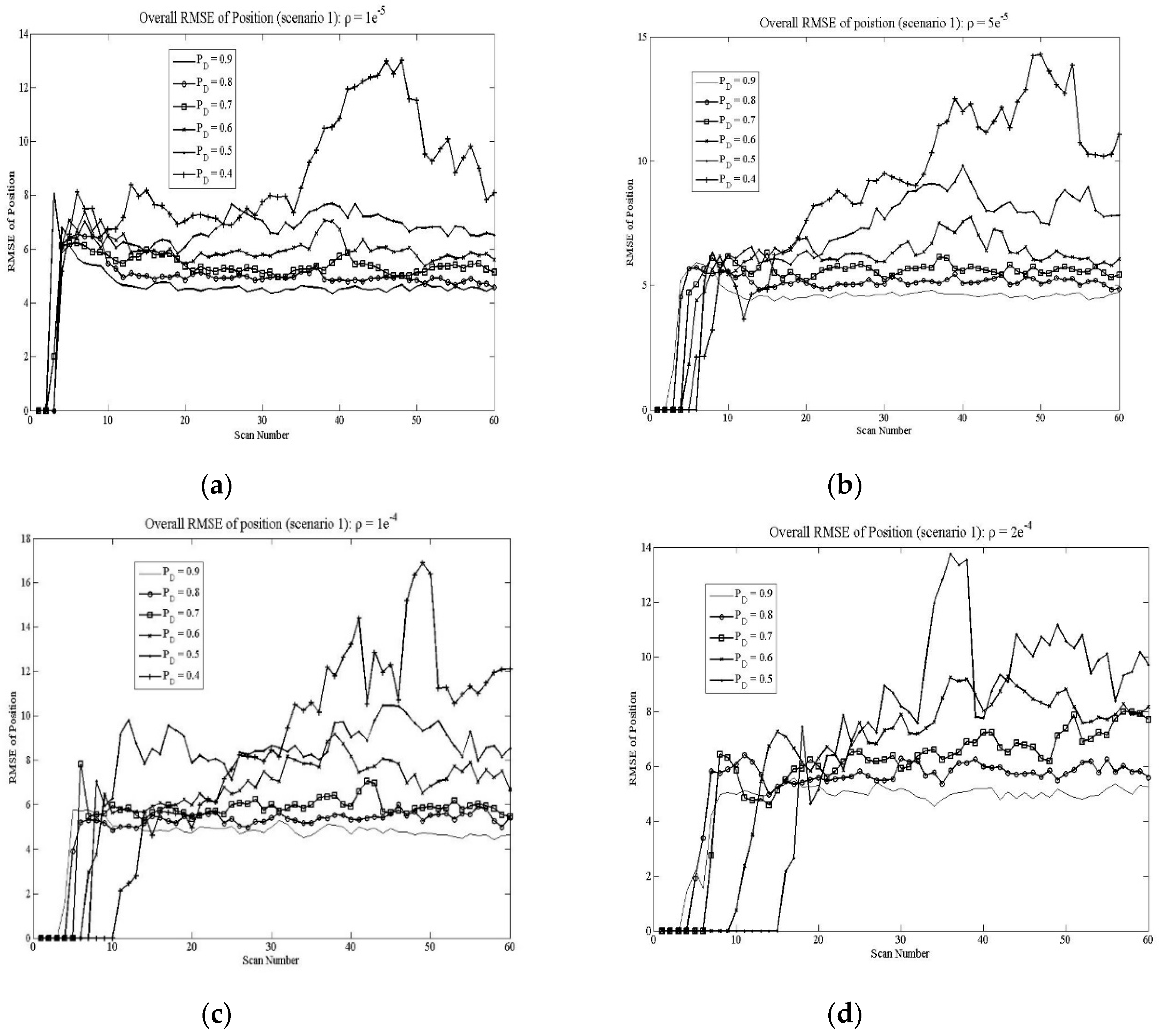
Figure 3. shows the RMSE of position (overall) diagrams for different clutter measurements parameters. A RMSE position error grows slightly, due to the appearance by the clutter density increasing.
Figure 3.
Overall RMSE of position (scenario 1): a) clutter density , b) clutter density , c) clutter density , d) clutter density .
Figure 3.
Overall RMSE of position (scenario 1): a) clutter density , b) clutter density , c) clutter density , d) clutter density .
4.2. Results of Simulations (Scenario 2)
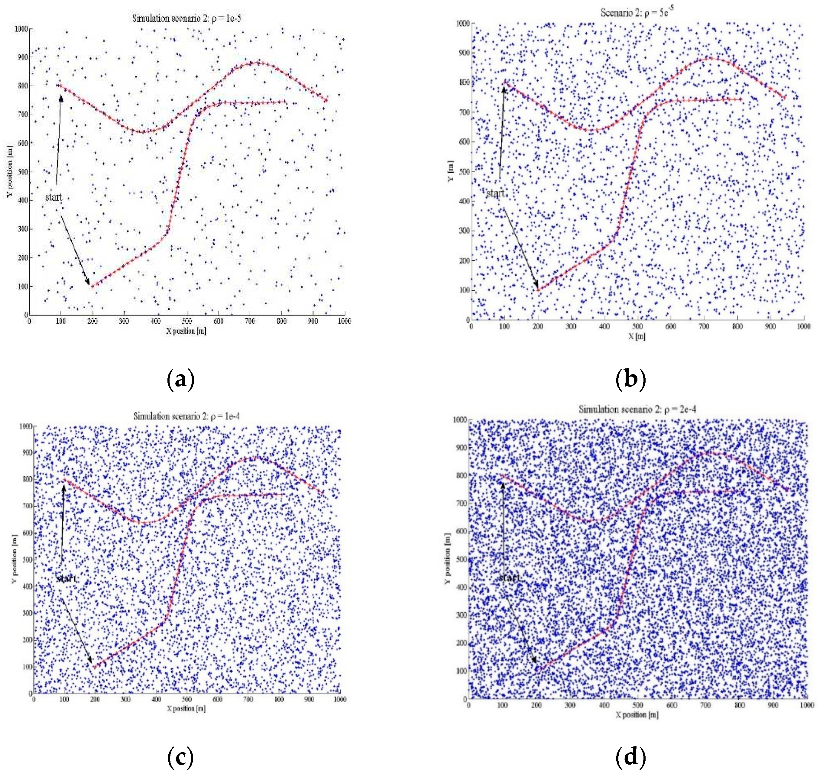
The second scenario contains a combined movement of the target (with a maneuver and without a maneuver). In this scenario, at beginning, both targets move in a straight line, at a constant speed, towards the center of the surveillance region, for 15 scans, after which they enter a left maneuver (CT) with an angular speed of pi/20, for duration of 6 scans.
Table 1.
Track parameters (scenario 1).
Table 1.
Track parameters (scenario 1).
|
PD
|
0.9 |
0.8 |
0.7 |
0.6 |
0.5 |
0.4 |
| 1e-5 |
faTrSum |
246 |
204 |
148 |
125 |
45 |
85 |
| coFaID |
281 |
171 |
109 |
57 |
20 |
22 |
| conTrPeak |
500 |
500 |
500 |
500 |
499 |
487 |
| Cpu |
0.59 |
0.63 |
0.67 |
0.69 |
0.63 |
0.67 |
| 5e-5 |
faTrSum |
86 |
105 |
61 |
45 |
12 |
52 |
| coFaID |
80 |
55 |
34 |
17 |
4 |
7 |
| conTrPeak |
500 |
500 |
500 |
499 |
485 |
373 |
| CPU time |
3.48 |
3.18 |
3.45 |
4.12 |
4.5 |
4.91 |
| 1e-4 |
faTrSum |
24 |
86 |
85 |
42 |
0 |
40 |
| coFaID |
26 |
28 |
17 |
8 |
0 |
4 |
| conTrPeak |
500 |
500 |
500 |
491 |
428 |
191 |
| CPU time |
7.00 |
7.54 |
9.8 |
10.3 |
11.2 |
11.3 |
| 2e-4 |
faTrSum |
24 |
79 |
50 |
4 |
27 |
- |
| coFaID |
14 |
21 |
9 |
2 |
2 |
- |
| conTrPeak |
500 |
499 |
492 |
409 |
212 |
- |
| Cpu |
16.1. |
16.5 |
16.9 |
16.8 |
17.8 |
- |
Then they continue in a straight line with a constant speed of 15 scans, after which they enter a right maneuver lasting 10 scans, with an angular velocity of pi/20. In the last 10 scans of the scenario, the targets continue to move in a straight line until the end of the scenario.
Figure 4.
Simulation scenario 2: a) clutter density , b) clutter density ,c) clutter density , d) clutter density .
Figure 4.
Simulation scenario 2: a) clutter density , b) clutter density ,c) clutter density , d) clutter density .
Table 2.
Targets tracking parameters (scenario 2).
Table 2.
Targets tracking parameters (scenario 2).
|
PD
|
0.9 |
0.8 |
0.7 |
0.6 |
0.5 |
| 1e-5 |
faTrSum |
966 |
1607 |
2644 |
4358 |
5568 |
| coFaID |
1062 |
1316 |
1282 |
1376 |
1150 |
| conTrPeak |
500 |
500 |
500 |
490 |
453 |
| Cpu |
0.51 |
0.55 |
0.6 |
0.63 |
0.68 |
|
PD |
0.9 |
0.8 |
0.7 |
0.6 |
0.5 |
| 5e-5 |
faTrSum |
1462 |
2673 |
4247 |
5669 |
5246 |
| coFaID |
1061 |
1225 |
1286 |
1101 |
608 |
| conTrPeak |
500 |
499 |
489 |
426 |
294 |
| CPU time |
2.93 |
3.21 |
3.45 |
4.17 |
4.53 |
| 1e-4 |
faTrSum |
1950 |
3615 |
4996 |
5353 |
2901 |
| coFaID |
1040 |
1185 |
1045 |
708 |
253 |
| conTrPeak |
499 |
482 |
435 |
333 |
253 |
| CPU time |
7.22 |
7.65 |
10.1 |
10.7 |
11.3 |
| 2e-4 |
faTrSum |
2929 |
4631 |
4559 |
2297 |
- |
| coFaID |
1059 |
961 |
602 |
187 |
- |
| conTrPeak |
490 |
440 |
303 |
126 |
- |
| Cpu |
16.6 |
17.1 |
17.1 |
18.3 |
- |
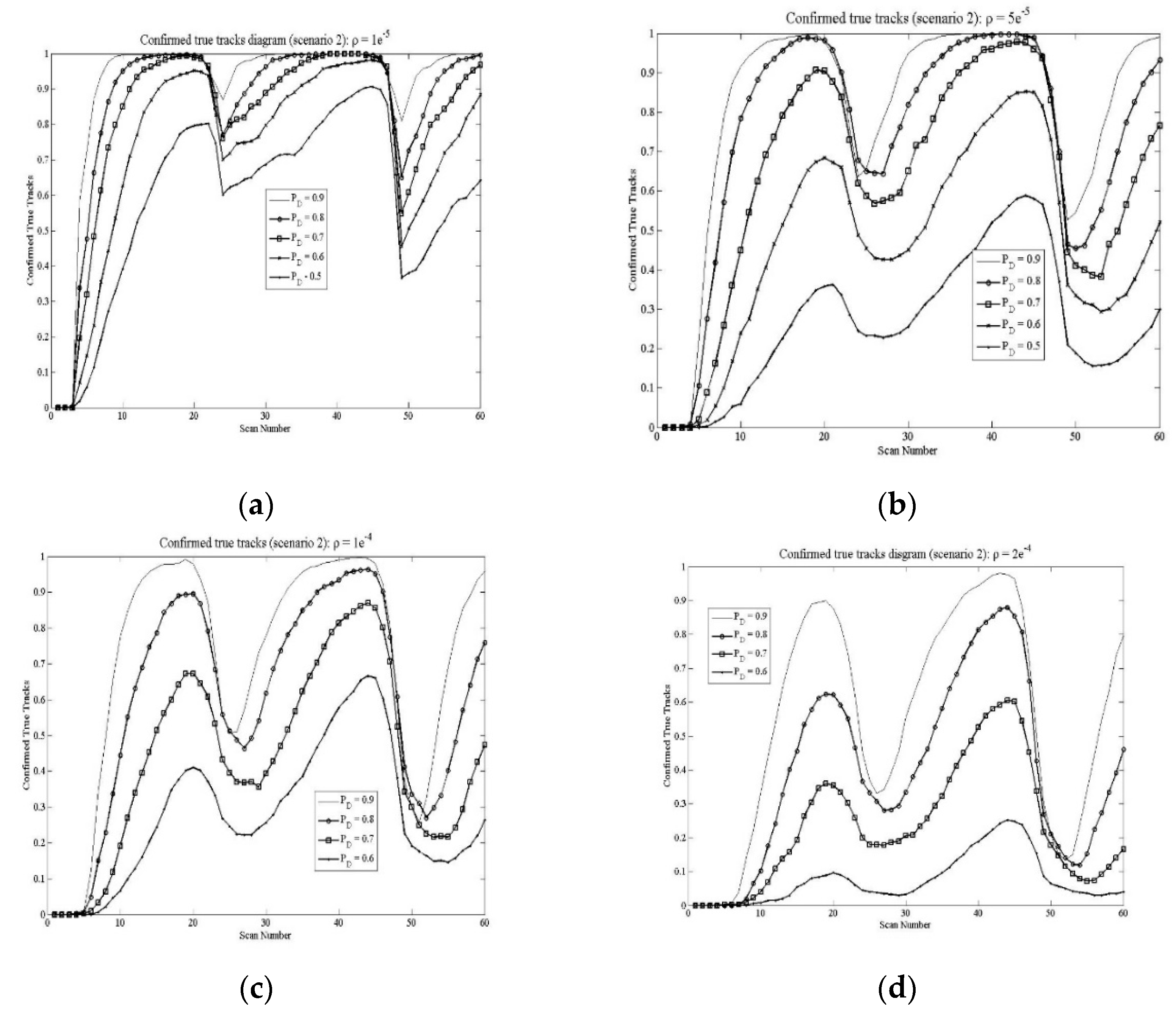
Figure 5.
Confirmed true tracks diagrams (scenario 2): a) clutter density , b) clutter density , c) clutter density , d) clutter density .
Figure 5.
Confirmed true tracks diagrams (scenario 2): a) clutter density , b) clutter density , c) clutter density , d) clutter density .
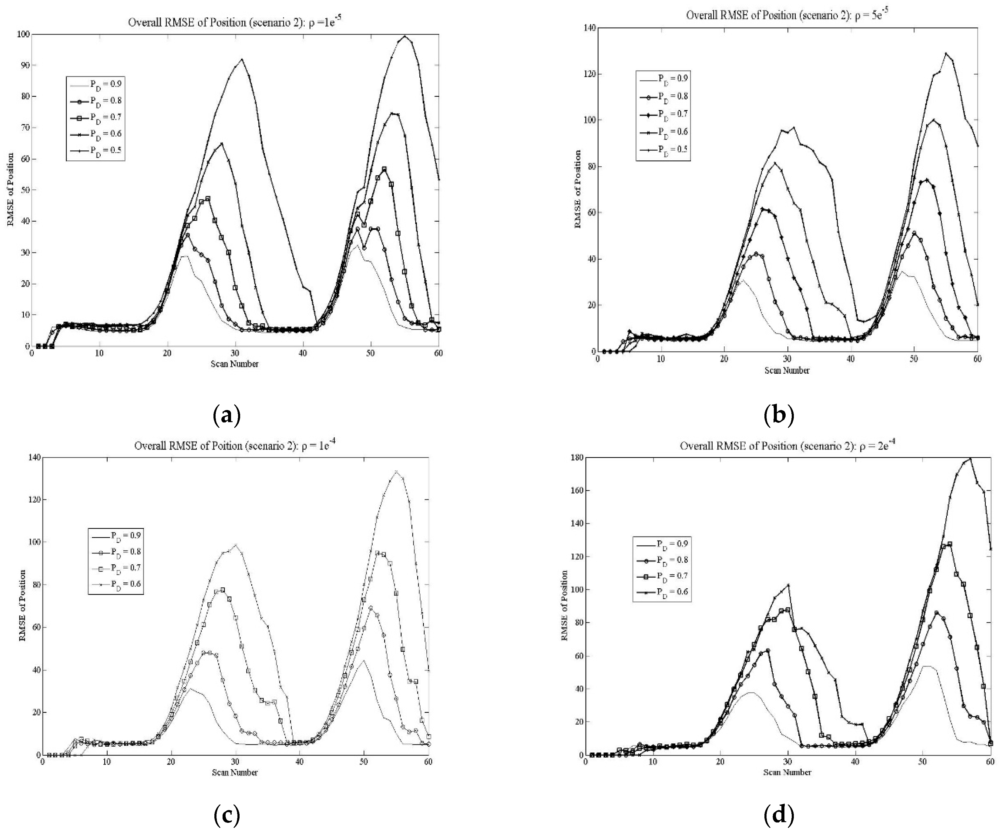
Figure 6. shows the RMSE of position (overall) diagrams for different clutter measurements parameters. A significant increase in the tracking RMSE error to the level of the impossibility of effective tracking is clearly highlighted, due to the appearance of maneuvers in the targetʹs trajectory and an increase in the density of clutter. It can be seen that clutter densities greater than
with a medium maneuver level indicate the end of effective tracking.
Figure 6.
Root mean square error position diagrams (scenario 2): a) clutter density , b) clutter density , c) clutter density , d) clutter density .
Figure 6.
Root mean square error position diagrams (scenario 2): a) clutter density , b) clutter density , c) clutter density , d) clutter density .
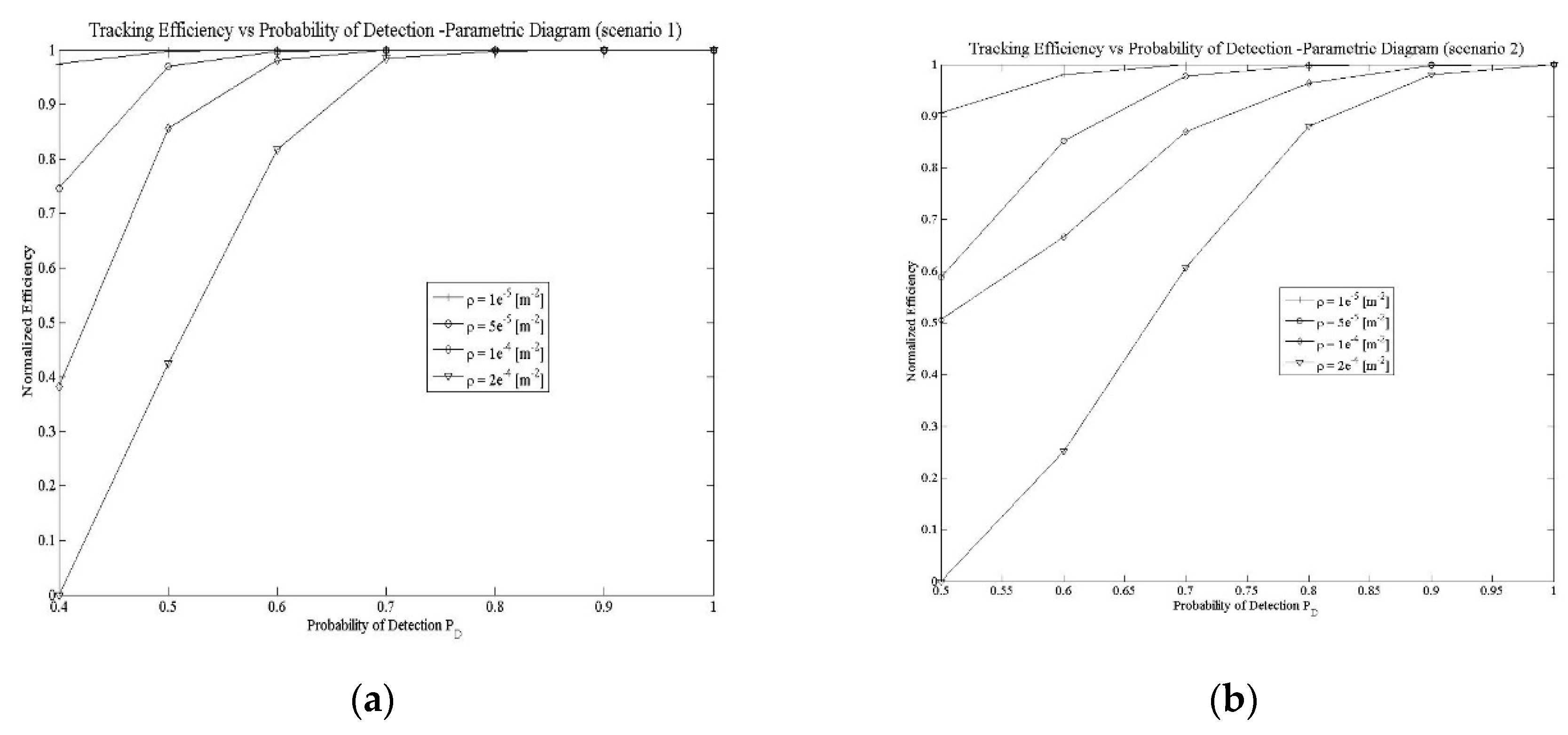
Figure 7. shows the normalized tracking efficiency versus probability of detection parametric diagram for both scenarios.
Figure 7.
Normalized tracking efficiency vs. probability of detection–parametric diagram a) scenario 1, b) scenario 2
Figure 7.
Normalized tracking efficiency vs. probability of detection–parametric diagram a) scenario 1, b) scenario 2
At
Figure 7.a), are given results of tracking efficiency for scenario 1. It can be seen that the ITS algorithm, for clutter density
measurements per scan has full performance for
PD = 0.8 while efficiency starts to drop at
PD = 0.7. For clutter density
measurements per scan ITS has full performance for
PD = 07 while efficiency starts to drop at
PD = 0.6. For clutter density
measurements per scan ITS has full performance for
PD = 0.6 while efficiency starts to drop at
PD = 0.5 and for clutter density
measurements per scan ITS perform full performance for
PD = 0.5 while efficiency starts to drop at
PD = 0.4.
At
Figure 7.b) shows normalized tracking efficiency versus probability of detection parametric diagram for scenario 2. The influence of the maneuver is evident, because the tracking results are weaker under the same tracking parameters. It can be seen that the ITS algorithm, for clutter density
measurements per scan has full performance for
PD = 0.9 while efficiency starts to drop at
PD = 08. For clutter density
measurements per scan ITS has full performance for
PD = 0.8 while efficiency starts to drop at
PD = 0.7. For clutter density
measurements per scan ITS has full performance for
PD = 0.7 while efficiency starts to drop at
PD = 0.6 and for clutter density
measurements per scan ITS perform full performance for
PD = 0.6 while efficiency starts to drop at
PD = 0.5.
Below these probabilities it is not possible to achieve fully automatic tracking of multiple maneuvering targets.
4. Discussion
Assuming that the target is effectively tracked in the part of the trajectory where the level of confirmed real tracks reaches the value 1, the user can conclude the following with respect to the known parameters of clutter density and detection probability:
- for a clutter density measurements per scan, targets in constant velocity (CV) motion mode can be efficiently tracked up to a detection probability of 0.4, while maneuvering targets can be efficiently tracked up to a detection probability value of 0.5.
- for a clutter density , targets in CV motion mode can be efficiently tracked up to a detection probability of 0.5, while maneuvering targets can be efficiently tracked up to a detection probability value of 0.6.
- for a clutter density measurements per scan, targets in CV motion mode can be efficiently tracked up to a detection probability of 0.6, while maneuvering targets can be efficiently tracked up to a detection probability value of 0.7.
- for a clutter density measurements per scan, targets in CV motion mode can be efficiently tracked up to a detection probability of 0.7, while maneuvering targets can be efficiently tracked up to a detection probability value of 0.8.
If target maneuvers are expected, it is necessary to include more target dynamic models, via the (for example) interacting multiple model - IMM algorithm.
5. Conclusions
The paper investigated and determining the limits of effectiveness for ITS -multi target tracking algorithm with different environment clutter density and probability of detection ability. The well-known ITS algorithm is given in theoretical and practical form and then its tracking efficiency is tested on different examples of clatter density and detection probability. The presented analysis and results provide the user with practical advice when choosing important parameters of the monitoring system. The values of the parameters in which the algorithm can still work efficiently are defined, so that the user has the opportunity to choose the optimal value of the tracking algorithm parameters. Extensive experiments showed that the dominant influence is the type of trajectory (with and without maneuver) and the density of clatter, while the probability of detection is a less significant parameter.
Further research should eliminate the influence of the maneuver (for example, using an interacting multiple model -IMM).
Author Contributions
Contributions to the conceptualization of manuscript, Zvonko Radosavljevic and Branko Kovacevic.; Contributions to the methodology and software, Dejan Ivkovic; validation and formal analysis, Dejan Ivkovic and Branko Kovacevic; investigation, resources, data curation, writing—original draft preparation, writing—review and editing, visualization, supervision, Zvonko Radosavljevic.; project administration, Mira Nikolic. All authors have read and agreed to the published version of the manuscript.
Funding
This work was supported by the Ministry of Science, Technological Development and Innovations (Serbia), Contract No. 451-03-47/2023-01/200325.
Data Availability Statement
No new data were created. Data is unavailable due to privacy or ethical restrictions. Suggested Data Availability Statements are available in section “MDPI Research Data Policies” at
https://www.mdpi.com/ethics.
Acknowledgments
The authors are thanked the Ministry of Science, Technological Development and Innovations (Serbia) and Ministry of Defense, Republic of Serbia. This work was supported by the Ministry of Science, Technological Development and Innovations (Serbia), Contract No. 451-03-47/2023-01/200325
Conflicts of Interest
The authors declare no conflict of interest.
References
- Bar-Shalom, Y.; Fortmann, T. E. Tracking and Data Association. Academic Press, San Diego, 1988. [CrossRef]
- Musicki, D., Evans, R. J.; Stankovic, S. Integrated probabilistic data association. IEEE Transactions on Automatic Control, 39, 6 (June 1994), 1237—1241.
- Reid, D. An algorithm for tracking multiple targets, IEEE Trans. AC, vol. AC-24, no. 6, pp. 843–854, 1979. [CrossRef]
- Song, T. L.; Mušicki, D.; Kim D.S.; Radosavljević, Z.; Gaussian mixtures in multi-target tracking: a look at Gaussian mixture probability hypothesis density and integrated track splitting, IET proceedings on Radar Sonar and Navigation, Vol 6, no 5, pp. 359-364, June 2012. [CrossRef]
- Radosavljević, Z. IPDA Filters in the Sense of Gaussian Mixture PHD Algorithm, Scientific Technical Review, 2016,Vol.66,No.3, pp.34-40, Belgrade 2016, UDK : 681:5.017:623:746.3, COSATI:17-09, 12-01. [CrossRef]
- Kurien, T. Multitarget Multisensor Tracking, vol. 1. Boston: Artech House, 1990, 43—83.
- Mušicki, D. Track score and target existence. In 9th International Conference on Information Fusion, Fusion 2006, Florence, Italy, July 2006.
- Mušicki, D., La Scala, B., and Evans, R. The integrated track splitting filter–Efficient multi-scan single target tracking in clutter. IEEE Transactions on Aerospace and Electronic Systems, 43, 4 (Oct. 2007), 1409—1425.
- Smith, P., and Buechler, G. A branching algorithm for discriminating and tracking multiple objects. IEEE Transactions on Automatic Control, 2, AC-20 (Feb. 1975), 101—104. [CrossRef]
- Bar-Shalom, Y., and Tse, E. Tracking in a cluttered environment with probabilistic data association. Automatica, 11 (Sept. 1975), 451—460. [CrossRef]
- Colegrove, S. B., and Ayliffe, J. An extension of probabilistic data association to include track initiation and termination. In Proceedings of the 20th IREE International Convention, Melbourne, Australia, 1985, 853—856.
- Davey, S. J., Gray, D. A., and Colegrove, S. B. A Markov model for initiating tracks with probabilistic multi-hypothesis tracker. In 5th International Conference on Information Fusion, Fusion 2002, Annapolis, MD, July 2002, 735—742. [CrossRef]
- Bar-Shalom, Y., Chang, K., and Blom, H. Multitarget Multisensor Tracking, vol. 1. Boston: Artech House, 1990, 25—42.
- Houles, A., and Bar-Shalom, Y. Multisensor tracking of a maneuvering target in clutter. IEEE Transactions on Aerospace and Electronic Systems, 25, 2 (Mar. 1989), 176—189. [CrossRef]
- Mušicki, D., Evans, R., and La Scala, B. Integrated track splitting suite of target tracking filters. In 6th International Conference on Information Fusion, Fusion 2003, Cairns, Queensland, Australia, July 2003. [CrossRef]
- Mušicki, D., and La Scala, B. Multi-target tracking in clutter without measurement assignment. IEEE Transactions on Aerospace and Electronic Systems, 44, 3 (July 2008), 877-896.
- Mušicki, D., Mallick, M., La Scala, B., Strange, S., and Evans, R. LMITS as an efficient MHT. In SPIE: Signal and Data Processing of Small Targets, vol. 5913, San Diego, CA, Aug. 1—4, 2005, OV1—OV12.
- Blackman, S., and Popoli, R. Design and Analysis of Modern Tracking Systems. Boston: Artech House, 1999.
- Lerro, D., and Bar-Shalom, Y. Interacting multiple model tracking with amplitude feature. IEEE Transactions on Aerospace and Electronic Systems, 29, 2 (1993), 494—509. [CrossRef]
- Ross, S. Stochastic Processes. New York: Wiley, 1983.
- Li, N., and Li, X-R. Tracker perceivability and its applications. IEEE Transactions on Signal Processing, 49, 11 (Nov. 2001), 2588—2604.
- Bar-Shalom, Y., and Li, X-R. Estimation and Tracking: Principles, Techniques and Software. Boston: Artech House, 1993. [CrossRef]
- Mušicki, D., and Evans, R. Joint integrated probabilistic data association–JIPDA. IEEE Transactions on Aerospace and Electronic Systems, 40, 3 (July 2004), 1093—1099. [CrossRef]
- Blom, H., and Bar-Shalom, Y. The interacting multiple model algorithm for systems with Markovian switching coefficients. IEEE Transactions on Automatic Control, 33, 8 (Aug. 1988), 780—783. [CrossRef]
- Fortmann, T., Bar-Shalom, Y., and Scheffe, M. Sonar tracking of multiple targets using joint probabilistic data association. IEEE Journal of Oceanic Engineering, 8, 3 (July 1983), 173—183. [CrossRef]
- Mušicki, D. Limits of linear multitarget tracking. In 8th International Conference on Information Fusion, Fusion 2005, Philadelphia, PA, July 2005.
- Mušicki, D., and Suvorova, S. Tracking in clutter using IMM-IPDA based algorithms. IEEE Transactions on Aerospace and Electronic Systems, 44, 1 (Jan. 2007), 111—127.
- Park S. Y., Song, T.L. Oh, R. and Choi, J.W. A new IMM interacting approach for unequal dimension states for multitarget tracking in cluttered environments, 2021 International Conference on Control, Automation and Information Sciences (ICCAIS), October 2021. [CrossRef]
- Ullah, I., Memon, S., Khan, U., and Song, T. L. (2022). Smoothing Linear Multi-Target Tracking Using Integrated Track Splitting Filter. Remote Sensing. 14. 1289. 10.3390/rs14051289. [CrossRef]
- Mušicki, D., and Evans, R. Clutter map information for data association and track initialization. IEEE Transactions on Aerospace and Electronic Systems, 40, 2 (Apr. 2004), 387-398. [CrossRef]
- Radosavljević, Z.; Ivković, D.; Kovačevic, B,: Integrated Particle Filter for Milti Target Tracking’, Proceedings of 8th International Conference of Electrical, Electronics, and Computing Engineering, IcETRAN 2021, Etno Village Stanisici, Republic of Srpska. Bosnia and Herzegovina, September 8-10, 2021.
- Kovačević, B,. Radosavljević, Z., Ivković, D. MHT and ITS: A Look at Single Target Tracking in Clutter, EUSAR 2018: 12th European Conference on Synthetic Aperture Radar Electronic Proceedings, 04 - 07 June, 2018, Aachen, Germany, pp 971-977. ISBN-10: 3800746360.
|
Disclaimer/Publisher’s Note: The statements, opinions and data contained in all publications are solely those of the individual author(s) and contributor(s) and not of MDPI and/or the editor(s). MDPI and/or the editor(s) disclaim responsibility for any injury to people or property resulting from any ideas, methods, instructions or products referred to in the content. |
© 2023 by the authors. Licensee MDPI, Basel, Switzerland. This article is an open access article distributed under the terms and conditions of the Creative Commons Attribution (CC BY) license (https://creativecommons.org/licenses/by/4.0/).
