Submitted:
13 July 2023
Posted:
14 July 2023
You are already at the latest version
Abstract
Overhead power transmission line icing (PTLI) disasters are one of the most severe dangers to power grid safety. Automatic iced transmission line identification is critical in various fields. However, existing methods primarily focus on the linear characteristics of transmission lines, employing a two-step process involving edge and line detection for PTLI identification. Nonetheless, these traditional methods are often difficult when confronted with challenges such as background noise or variations in illumination, leading to incomplete identification of the target area, missed target regions, or misclassification of background pixels as foreground. We propose a new iced transmission line identification scheme to overcome this limitation. In the initial stage, we integrate the image restoration method with image filter enhancement to restore the image's color information. This combined approach effectively retains valuable information and preserves the original image quality, thereby mitigating noise presented during the image acquisition. Subsequently, in the second stage, we introduce an enhanced multi-threshold algorithm to separate background and target pixels. After image segmentation, we enhance the image and obtain the region of interest (ROI) through connected component labeling modification and mathematical morphology operations, eliminating background regions. Our proposed scheme achieves an accuracy value of 97.72%, a precision value of 96.24%, a recall value of 86.22%, and the specificity value of 99.48% based on the average value of test images. Through object segmentation and location, the proposed method can avoid background interference, effectively solve the problem of transmission line icing identification, and achieve 90% measurement accuracy compared to manual measurement on the collected PTLI dataset.
Keywords:
power transmission line icing
; icing thickness
; transmission line identification
; multi-threshold
; image restoration
; connected component labeling
1. Introduction
The development of the intelligent grid increases the design, operation, and maintenance requirements for power transmission lines. However, transmission lines are susceptible to icing at low temperatures, high air humidity, and precipitation. Extreme power system failures can be caused by ice loads, wind loads, and dynamic oscillation, such as cable rupture, tower failure, and transmission line galloping [1,2,3,4,5,6]. Therefore, an effective monitoring and predictive alarm system for power transmission line icing (PTLI) is important for ensuring the safety of the power grid. Traditional PTLI monitoring techniques, such as artificial inspection [7], the installation of pressure sensors [8], and the development of meteorological models [9], among others, have been extensively employed to achieve this objective. In recent years, PTLI monitoring based on computer vision methods has emerged as a new research direction [10] that makes icing monitoring visible, practical, and cost-effective. Several algorithms based on 2D, such as adaptive threshold segmentation [11], edge extraction [12], and wavelet analysis [13], are presented in order to obtain accurate ice edge information. The ice thickness can be calculated by comparing the pixel dimensions between edges in normal and icing conditions. However, these algorithms perform poorly in complex contexts or situations with limited exposure. Furthermore, the 2D estimation method cannot obtain comprehensive information about ice thickness. Methods based on 3D measurement have been introduced to monitor PTLI to obtain more accurate information about icing to address this issue. The PTLI monitoring based on binocular vision mainly includes camera calibration, transmission line identification, key point matching, and ice thickness calculation.
The identification of transmission line icing is an important part of PTLI monitoring. At this stage, the goal is to identify the top and bottom of the iced transmission line so that it will directly affect the ice thickness measurement. Generally, the iced transmission line identification stage consists of two stages, namely edge detection and line detection. Edge detection accuracy is related to low contrast, cluttered backgrounds, occlusion, and the image quality obtained by the camera [14]. When a PTLI image is acquired, background and illumination factors affect the image environment and transmission process. The image of the transmission line identification process applies the compression method, leading to icing images with low contrast characteristics, complex grayscales, all kinds of noises, Etc. [15,16]. Based on the above reasons, finding an accurate edge detection method for iced transmission line identification is crucial. According to previous researchers, conventional edge detection operators have categories, such as first-order derivative or gradient-based (Roberts, Prewitt, and Sobel) [17]. Conventional edge detection methods use low-level signs such as colors, brightness, textures, and gradients in the images [18]. However, there is a need for more accuracy to meet the application requirement. Traditional Canny and Hough transforms have often been applied to identify line icing [6], with Canny operators for edge detection of line icing and Hough transforms for straight lines [19,20]. However, this method has interference noise, so other objects are sometimes detected. The lighting in the image also has a significant impact on this conventional edge detection [3]. The Canny edge detection algorithm has a few things to improve, such as broken edges [21,22]. Many edges of objects in the background are also detected. In this case, it will be a challenge to distinguish which object (the iced transmission line) is selected and which is the background. Zhang et al. [23], proposed an edge detection of the icing image of the transmission line based on the wavelet transform and the morphology fusion. The image background and noises easily disrupt the edge detection identification result.
Based on the problems above, the main works and innovations proposed in this paper include:
- Aiming at the problem that iced transmission line detection is easily affected by background and noise, an image optimization method is proposed, which combines the image restoration method and image filter enhancement to alleviate the influence of noise and light.
- An enhanced multilevel threshold algorithm is proposed to segment background and target pixel areas.
- Connected component labeling modification and mathematical morphological operations are used to refine the segmentation image, obtain the ROI, and determine the position of the top and bottom of the line.
This paper is organized as follows: Section 2 summarizes PTLI identification and extraction. Section 3 illustrates the proposed method for transmission line icing identification. Section 4 introduces our proposed ice thickness calculation by 3D measurement. Section 5 presents the experimental results and discussion. In addition, Section 6 states the conclusions and future work.
2. Transmission Line Icing Identification
The main problem with PTLI monitoring based on binocular vision is iced transmission line identification and extraction, which directly affects automation and monitoring intelligence. The target detection algorithm identifies and extracts the transmission line icing image. However, the environment of PTLI is generally complex, and there is interference information, such as background and noise, in the collected images. In PTLI identification, the accuracy of the traditional edge and line detection algorithm is still insufficient, and the noise interference from the PTLI image is substantial. The high similarity of color and texture makes its detection and identification more difficult. Therefore, it is necessary to design a reliable scheme for iced transmission line identification.
3. New Scheme for Iced Transmission Line Identification
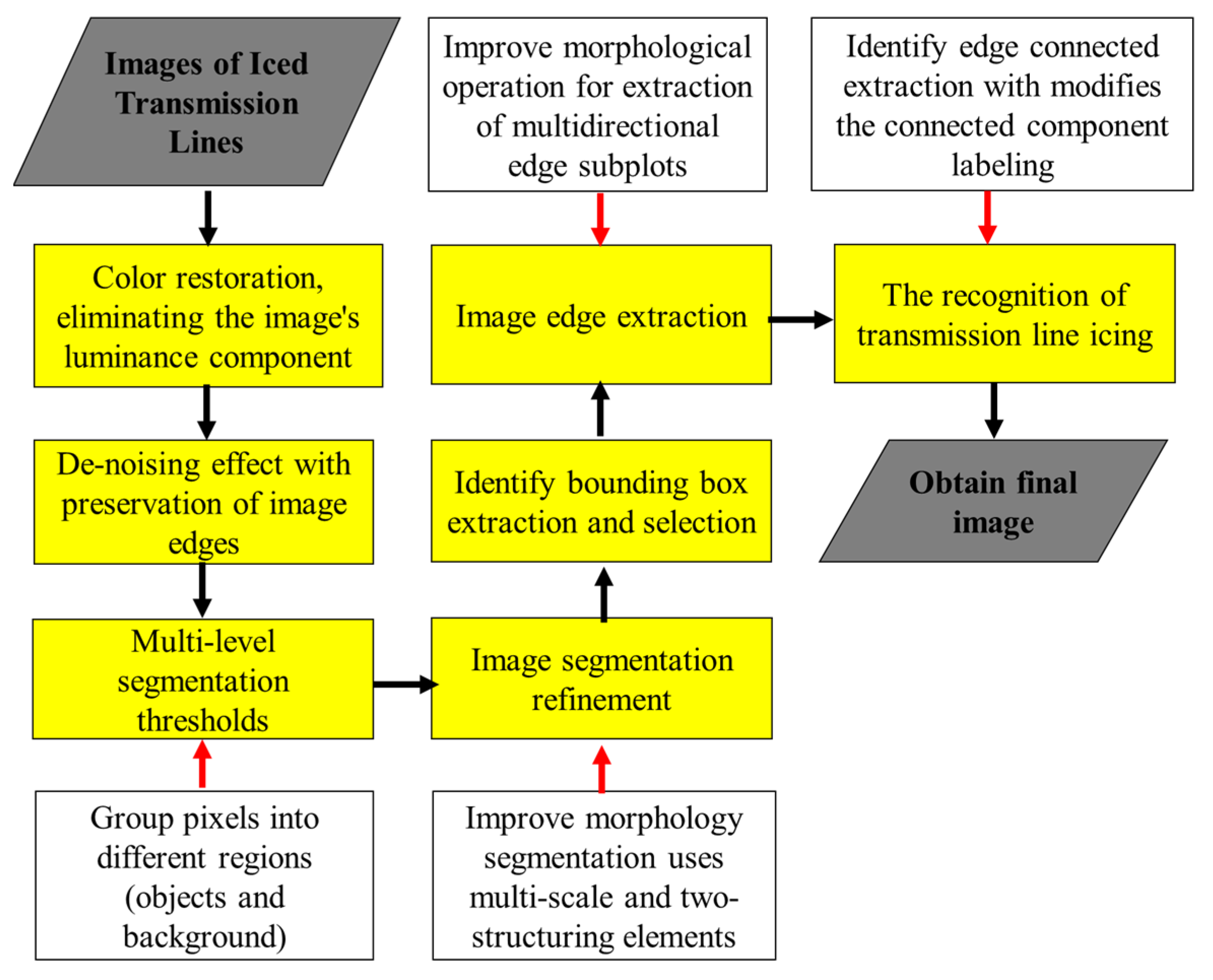
This paper proposes a reliable iced transmission line identification scheme to overcome difficulties with PTLI identification. Figure 1 shows our proposed scheme for iced transmission line identification. We integrate image restoration techniques with image filter enhancements in the early stages. This stage solves problems such as increased noise in the original image, dim and dark images, and a grayish tint in the original image. In addition, image filter enhancement is proposed to remove unwanted noise during image acquisition and retain valuable information, such as the edges of the transmission line and the texture of the icing lines. PTLI images often blend with other objects, or noise appears during image processing even though the background is simple. Therefore, the next stage is an enhanced multilevel segmentation threshold algorithm to segment background and target pixel areas. The results of multilevel threshold images contain gaps and holes, so modification morphological operation is added to improve segmentation results by utilizing two multiscale and mathematical two-structuring elements. We improve the image and obtain the region of interest (ROI) based on bounding box identification for eliminating background regions. After object segmentation and localization, the next step is PTLI edges identification. Mathematical morphology is proposed at this stage to extract multidirectional edge subplots and smooth the region. Finally, modified connected component labeling is proposed to identify the top and bottom iced lines. This modification reduces the processing time and memory space required to analyze neighboring pixels. A more detailed explanation of the stages in iced transmission line identification is explained in the sub-section below.
Figure 1.
The new scheme of iced transmission lines identification and extraction.
3.1. Image Color Restoration
The Materials Images taken by cameras often appear dim and unclear, then it has distorted hues from their true colors. Likewise, the appearance of color in recorded images is strongly influenced by spectral shifts in the scene illumination. The reason has two aspects; on the one hand, insufficient light prevents the camera from gathering enough information. On the other hand, the dynamic range of a camera is much narrower than the human visual system. Some of the iced transmission line images used in this study appear dim and unclear, then the images have distorted hues from the original color, so restoring the original image before going to the next stage is needed. Retinex (Retina+Cortex) is an enhancement technique that attempts to attain color constancy. The Retinex modification is used to enhance the image's color. Figure 2 shows a block diagram for image color restoration, and Table 1 shows the color restoration algorithm.
Figure 2.
Block diagram for image color restoration.
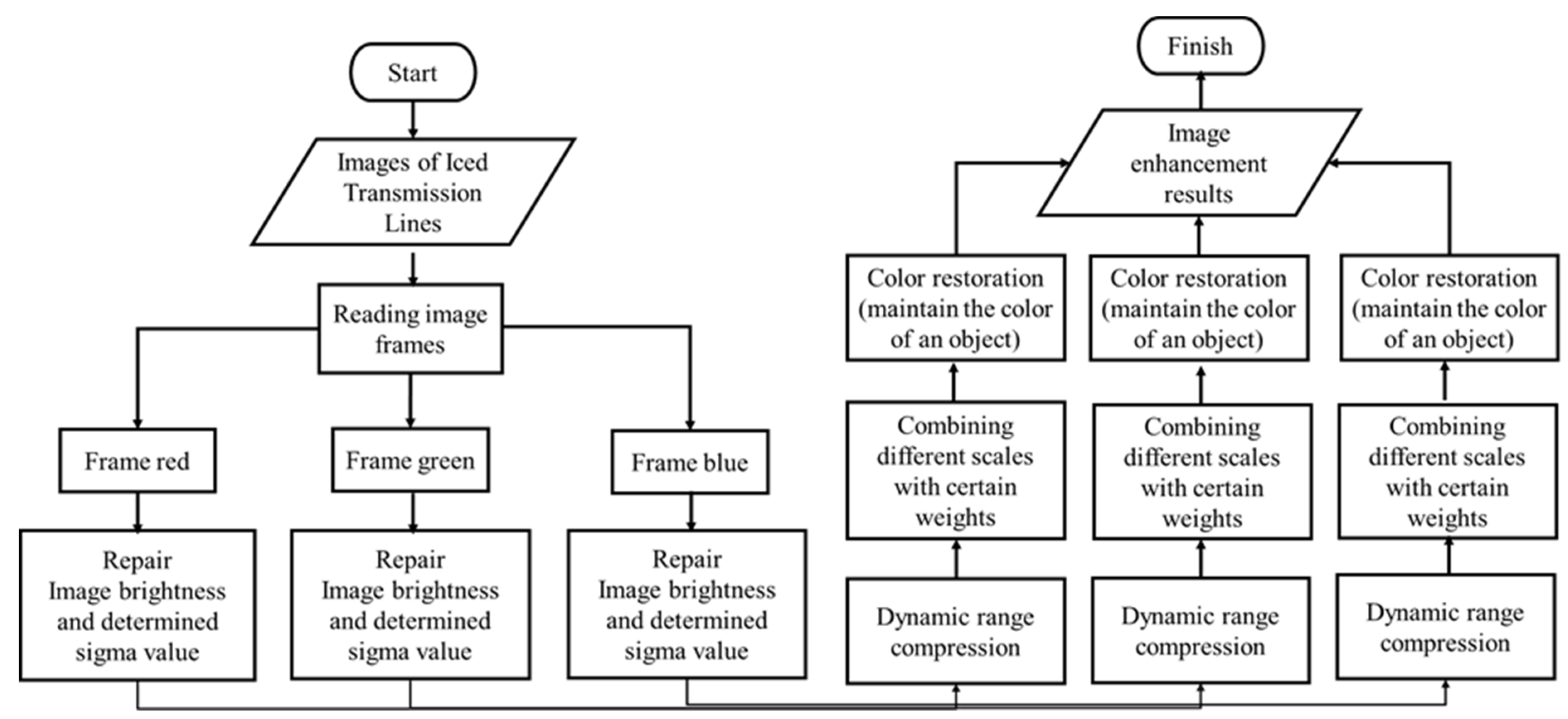
According to Figure 2, the PTLI images for the experiment are prepared for the initial steps, then all frames are read from the image. The frames are classified into red, green, and blue. The Gaussian surround is calculated after the image frame is read. Gaussian surround is used as a filter to smooth out the original image. The formula used is as follows.
The following is an explanation of Equation (1):
: Gaussian on pixels
: Exponential;
: Pixel coordinates;
: Sigma value
The first step uses the Gaussian surrounding to increase the image's brightness. This stage is intended for image smoothing beforehand. The Gaussian value is obtained from Equation (1) and uses three sigma values. The procedure is performed to enhance the image's brightness. Gaussian value is determined using three sigma values. The three sigma values used are. However, this value can be changed as needed. Table 2 shows the color restoration algorithm. After the image brightness increases, the next stage is the original image matrix combined with the Gaussian kernel. The image matrix for each color channel was used as the original image matrix. The detail in dark areas is enhanced by small sigma. At this stage, a member of the class functions center/surround, where the output is defined by the difference between the input value (center) and the average of its environment (surround).
The general mathematical form is as follows:
where, the input image on the color channel, output image on the channel, and is the normalized surround function. This stage is performed on each color channel. The formula used for convolution calculations is as follows:
The following is an explanation of the convolution formula:
: Gaussian on pixels
: Convolution
: Image matrix
: Color channels (R, G, and B)
Different scales are combined with specific weights at a later stage. The initial stage of this method is to determine the weight to be used. Each weight will be multiplied by the results of each convolution matrix and then added up. Weight values can be adjusted according to the requirements. It affords an acceptable trade-off between a good local dynamic range and a good color rendition. The output is defined as a weighted sum of the outputs of several previous stages (dynamic range compression). The Equation of this stage is as follows:
where N is the number of scales, is the weight of each scale.
The last step in image enhancement is the image quality related to the image's brightness, which is improved by maintaining the color firmness. The concept of color constancy or determination is derived from the human vision system, which attempts to maintain the appearance of an object's color under varying illumination conditions. The chromaticity coordinates are calculated in the first step.
For the color band, where is the number of spectral channels (Generally, for RGB color space. The restored color is given by
where,
The band of the color restoration function (CRF). The best overall color restoration is defined by
For the channel, at positionCRF depends on the ratio composition of the pixel at for that channel value to the total of all of them. Where is a gain constant, and controls the strength of the normality. A set of and values that work for all spectral channels (RGB) is determined by experiment [24]. and are constants, taken at 46 and 125, respectively [24].
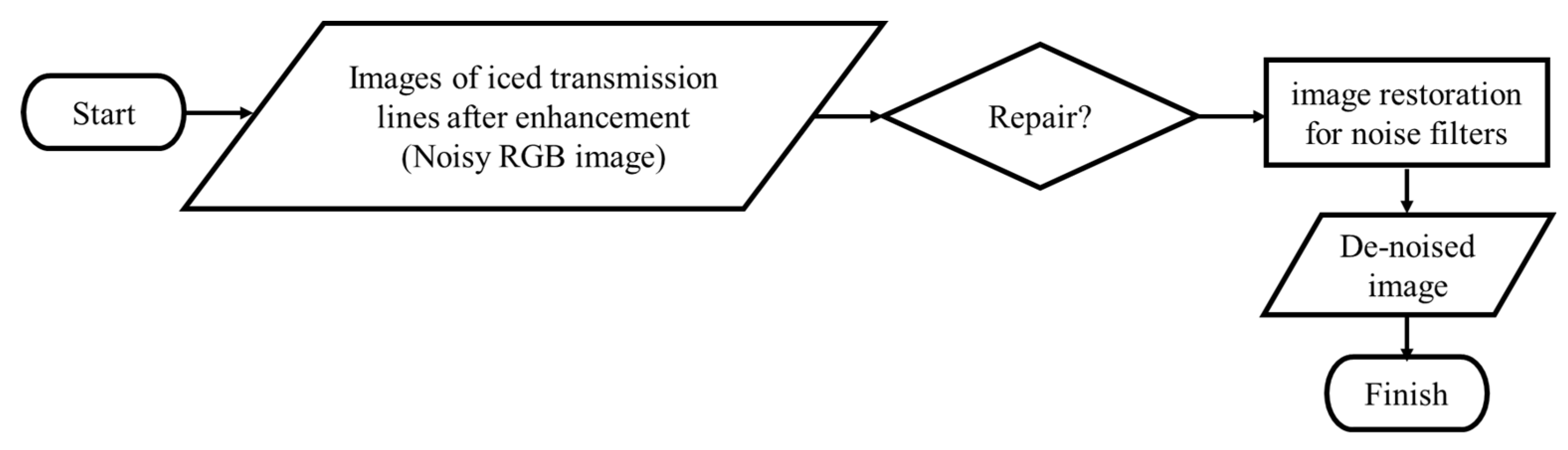
3.2. Image De-noising
Figure 3 shows the block diagram of image de-noising. Based on the block diagram in Figure 3, the input data from this system is the PTLI image that has been restored in color. The color-corrected image still contains noise, so a filter is needed to remove noise and retain critical information in the image. If the image color restoration stage focuses on lighting and color restoration, this stage focuses on image filter from noise. After the PTLI image data is prepared, the image containing noise will be restored. Then the output from this system is a de-noising image while maintaining the edges of the transmission line. The Gaussian smoothing concept focuses on filter coefficients enhanced in this method by relative pixel intensities. This method obtains the resulting image pixel values from the weighted average of neighboring pixels through a convolution process. The smaller the pixel's spatial weight, the greater the pixel distance to the central pixel analysis in an image, and vice versa. The more significant the difference in intensity between two pixels, the smaller the photometric weight, so the contribution to the weighting is small. Three parameters control this filter method: kernel dimension, standard deviation to control factors of spatial weighting, and standard deviation to control factors of photometric weighting.
Figure 3.
The block diagram of image de-noising.
Spatial weighting in this filter means giving weight to pixels according to the distance between the pixel and those that are the center of analysis in the image. Spatial weight (WS) is the realization of measuring spatial proximity in a Gaussian function that measures the spatial distance between pixels using Euclidean distance. The calculation of the spatial weight for each pixel is shown in Equation (9).
With:
: Spatial weight of each pixel in the kernel;
: Kernel midpoint (w (0, 0));
: Neighbouring elements in the kernel;
: Standard deviation for weighting spatial
Meanwhile, photometric weighting means that the weighting of pixels is based on the size of the difference in the pixel's intensity with the pixel's intensity that is the center of analysis in the image. Photometric weight (WR) is the realization of measuring the difference in intensity based on the photometric similarity in the Gaussian function, which measures the difference in intensity between pixels using the Euclidean distance. The calculation of the photometric weight at each pixel is shown in the following Equation.
With,
: Photometric weight per pixel in the kernel
: Kernel midpoint (w (0, 0));
: Neighbouring elements in the kernel;
: Pixels, which are the center of analysis in degraded images;
: Neighbouring pixels of pixel g[x];
: Standard deviation for weighting photometric.
The two weights (spatial and photometric weights) are normalized to one weight value (W) as in Equation (10).
After the weighting of the pixels is done, the resulting pixel values can be found in Equation (11).
With,
: Neighbouring weight values in the W weight matrix;
: The calculated pixel value.
3.3. Multi-leve Threshold
This subsection explains a multilevel segmentation threshold that marks out the targets of interest in an image. The goal at this stage is to separate the transmission line icing pixels from the background. The selection of thresholds is critical and related to the good or bad results after segmentation. With proper segmentation, an image can be described simply by utilizing meaningful things, which are easier to analyze. A multilevel segmentation threshold is a process that splits the degree of grey in an image into transparent regions based on several points or threshold values. A multilevel threshold separates pixels into classes or groups. Pixels in the same class will have a degree of grayscale within a specific range obtained from several thresholds. Figure 4 shows a block diagram of the multilevel threshold segmentation process.
Figure 4.
The block diagram of the multilevel threshold segmentation process.
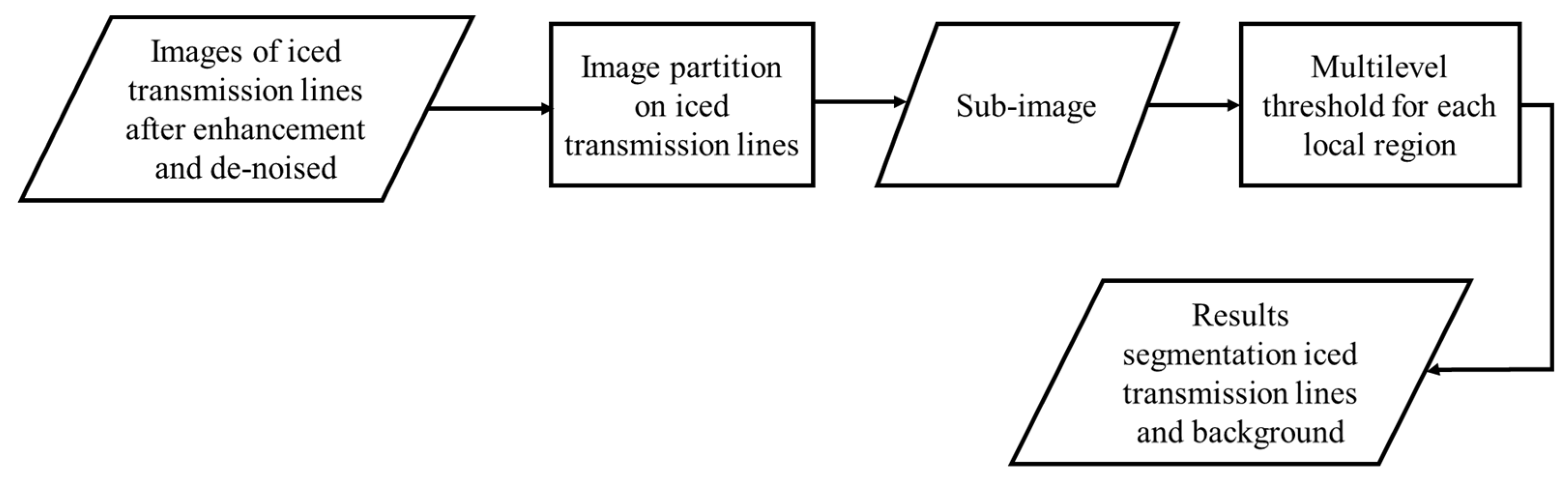
Initially, the input image is divided into several sub-images. In the next stage, a multilevel threshold is applied based on the histogram information of each sub-image. Two local threshold values divide the image into two regions: the transmission line icing and the background. The local threshold value is the threshold value for each sub-image. The process is repeated until all sub-images are segmented. Figure 5 shows in detail the multilevel threshold process.
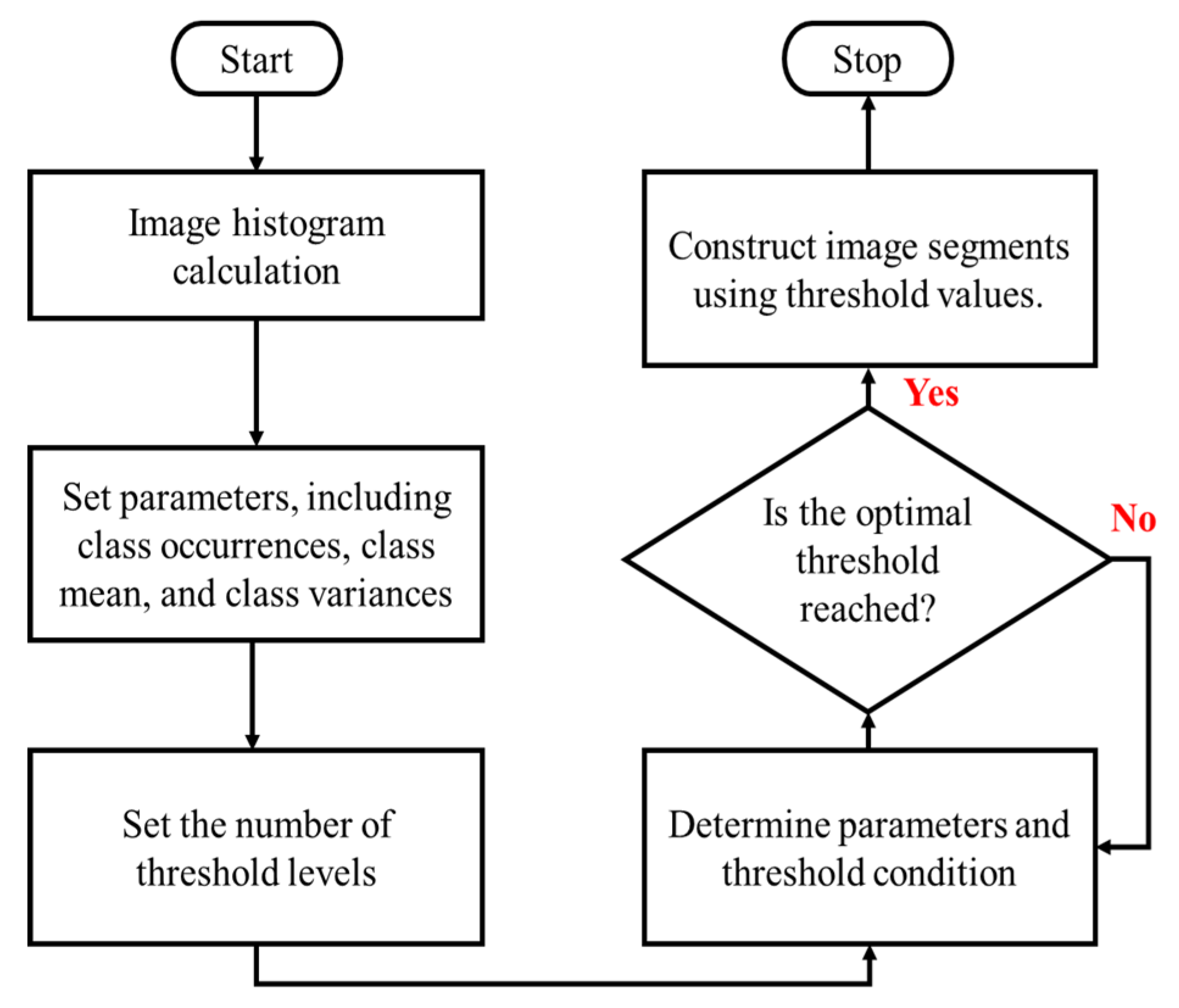
Figure 5.
The block diagram of the multilevel threshold for each local region.
The pixels of the image are separated to a good number of levels of preferred thresholds. The image is sectioned into levels or classes, which are denoted by and . Consequently, the class occurrences , the mean class levels and class variances respectively are computed as in (14), (15), and (16).
The within-class variances of all segmented classes of pixels is given as (17).
The between-class variances measure the spare ability among all classes (18).
The process is repeated until all sub-images are segmented. Figure 14 shows in detail the multilevel threshold process.
3.4. Mathematical Morphology
There are many kinds of operators in mathematical morphology, among which the most basic ones are dilatation and erosion. The opening and closing operations are two critical secondary operations based on the dilatation and erosion operations. The morphological calculation process from a mathematical perspective is as follows:
It assumes that Ω represents the two-dimensional Euclidean space. B is a mathematical structural element that operates with, where and are subsets of Ω. Φ represents empty sets. Erosion operation (sometimes called "Minkowsky subtraction") is defined as follows:
Based on Equation (19), represent erosion of A. Erosion of by means that contains the set of all points in after B translates. Corrosion is an operation that shrinks or refines A. Dilation operation (sometimes called "Minkowsky addition") is defined as follows:
Which represents the expansion of B to A. The operator is the structural element of B's origin image. The expansion of B to A refers to the set of all displacements x based on the translation of the image structure element x. Dilation refers to growing or coarsening pixels in a binary image. Opening and closing are critical morphological filters for image smoothing, which is good for smoothing light and dark image features. These smoothed features could be extracted for image analysis. However, based on the characteristics of the transmission line icing image used in this research, it only uses a closing operator to maintain its edge contour. The closing operation for the filter is described as follows:
Equation (21) means that element B first dilates A, and then B erodes the result.
When the morphology is applied in the image processing, A is to process the image, and B is a structural element. The gaps and holes are connected to the neighboring objects and smooth objects. In addition, both operations will not significantly change the image area or shape. The binary image obtained after the segmentation threshold contains a transmission line covered with iced targets, background, and other interference objects. Besides that, the segmentation result of the transmission line is still rough, so it is necessary to enhance the object. Mathematical morphology is a nonlinear filtering method; applied mathematical morphology can simplify image data to maintain its essential shape characteristics. In most cases, a single structural element realizes the mathematical morphology, which makes edge detection of transmission line effects poor. A single structural element can only detect edge structural element information in the same direction, while the other directions are not edge-sensitive.
Morphological operations are applied on segmented images for smoothening the image. The mathematical morphology has been enhanced in this study. Figure 6 shows a flowchart for image segmentation refinement using mathematical morphology.
Figure 6.
The flowchart for image segmentation refinement using mathematical morphology.
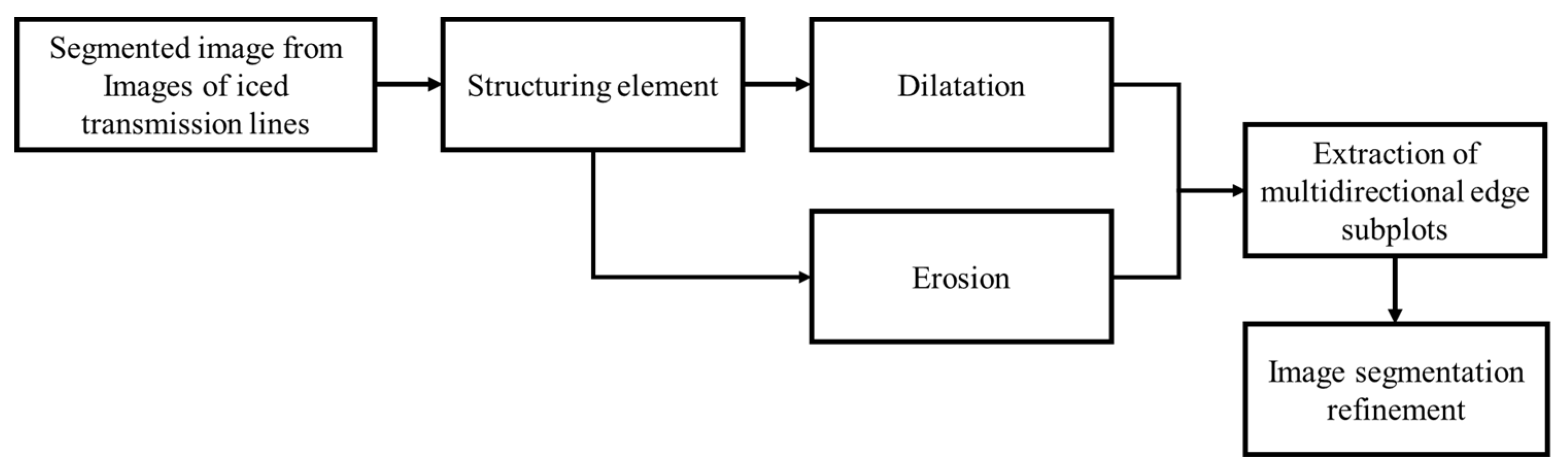
The scheme extended a compromise method, which uses multiscale and two structuring elements for alternating sequences of morphological opening and closing filtering to smooth the image and remove the noise. It effectively solves the problems posed by single structural elements. Morphological edge detection operator with multiscale elements and two structuring elements, where is the gray image, is the structuring element:
Where and respectively, are diamond-type structuring elements and cross-shaped structuring elements.
and are structural elements with different scales. Although the ability to eliminate noise is weak, small-scale structural elements can better retain image edge information. Large-scale structural elements can remove image noise well but miss some transmission line edge information. So multiscale structure elements and two structures can effectively remove image noise and retain good line-icing segmentation result information. This improved mathematical morphology removes small dark spots and connects small bright cracks. Otherwise, it is used to close the dark gaps between light features.
3.5. Bounding Box Identification
This feature can separate certain areas of the PTLI image that are considered more important than other objects. In the PTLI image with ROI coding, that area will have higher image quality than the background.
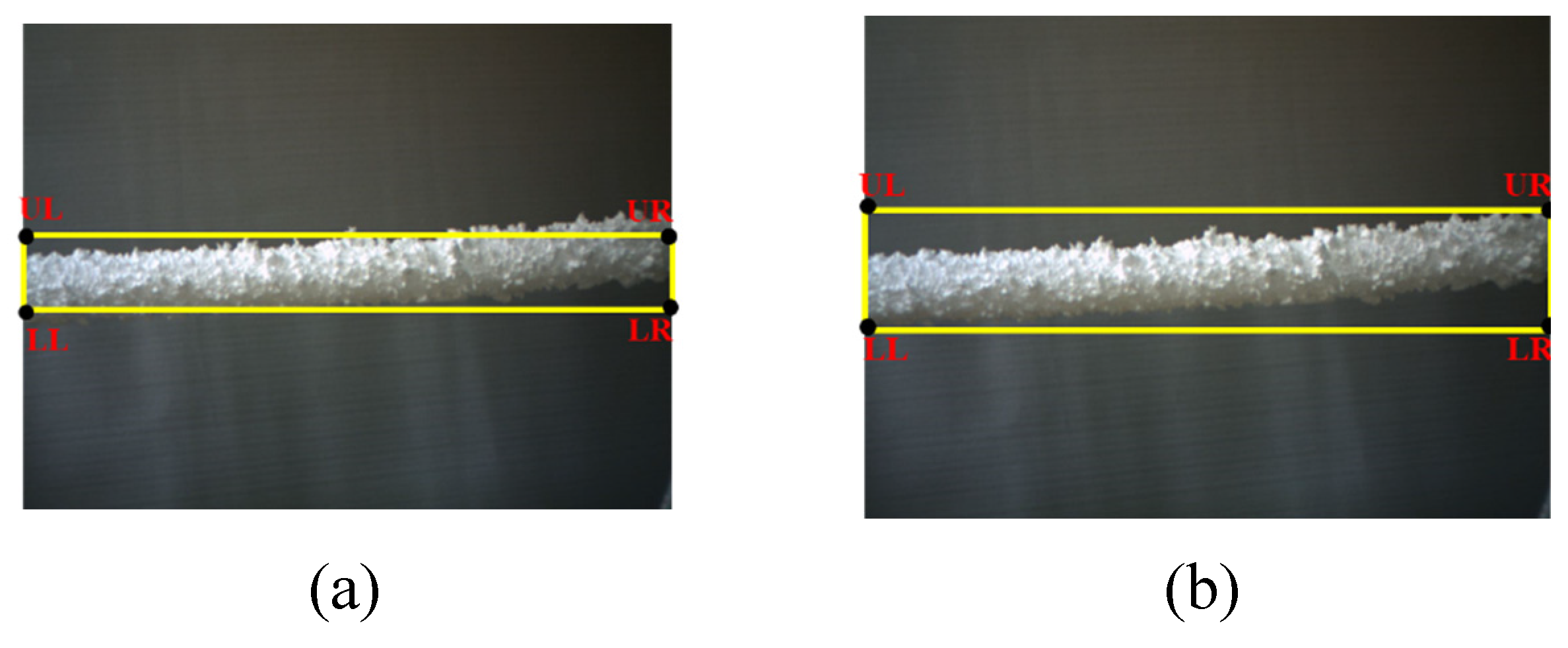
The method for determining the bounding box is if the iced transmission line forecast image is , then are the connected components (regions) contained in , with ; is the number of regions; or . A bounding box is obtained for each based on the line icing forecast image. A bounding box is an imagined box that encloses a specified area that surrounds. The bounding box for each is determined based on the spatial coordinates of the upper-left (UL), upper-right (UR), lower-left (LL), and lower-right (LR) pixels. Suppose the size of the image is, where M is the number of pixel rows, and N is the number of pixel columns. Then the illustration of the bounding box is shown in Figure 7. The flow of determining the bounding box for each region is shown in Figure 8. Yellow boxes indicate connected component bounding boxes (regions). The bounding box obtained only surrounds the transmission line icing area (Figure 8 (a)). The bounding box's size is once more adjusted by widening it to cover the entire area of the line icing. Each bounding box spatial coordinate (UL, UR, LL, LR) is widened by adding k pixels (Figure 8(b)). The k value is obtained from the average iced transmission line pixel width.
Figure 1.
Illustration of bounding box identification. (a) RGB Image; (b) Describe an image in pixels.
Figure 1.
Illustration of bounding box identification. (a) RGB Image; (b) Describe an image in pixels.

Figure 8.
The Flow of Bounding Box Determination.
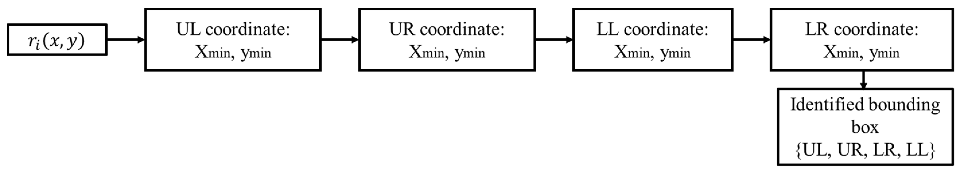
Figure 9.
Bounding box. (a) The bounding box before widening; (b) The bounding box after extended with k pixels in size.
Figure 9.
Bounding box. (a) The bounding box before widening; (b) The bounding box after extended with k pixels in size.
3.6. Image Edge Extraction
The results of line icing segmentation were obtained in the previous stage by selecting the region of interest. After the segmentation process, the edge detection results are still unclear, so improving the mathematical morphology used to emphasize the object's shape (transmission line icing) is necessary. At this stage, the PTLI image edge extraction will be explained. Mathematical morphology is also used for the extraction of line-icing edges. In this method, the focus is on enlarging bright regions and shrinking dark regions. Figure 10 shows the block diagram for edge extraction using improved mathematical morphology.
Figure 2.
The block diagram for edge extraction using improved mathematical morphology.
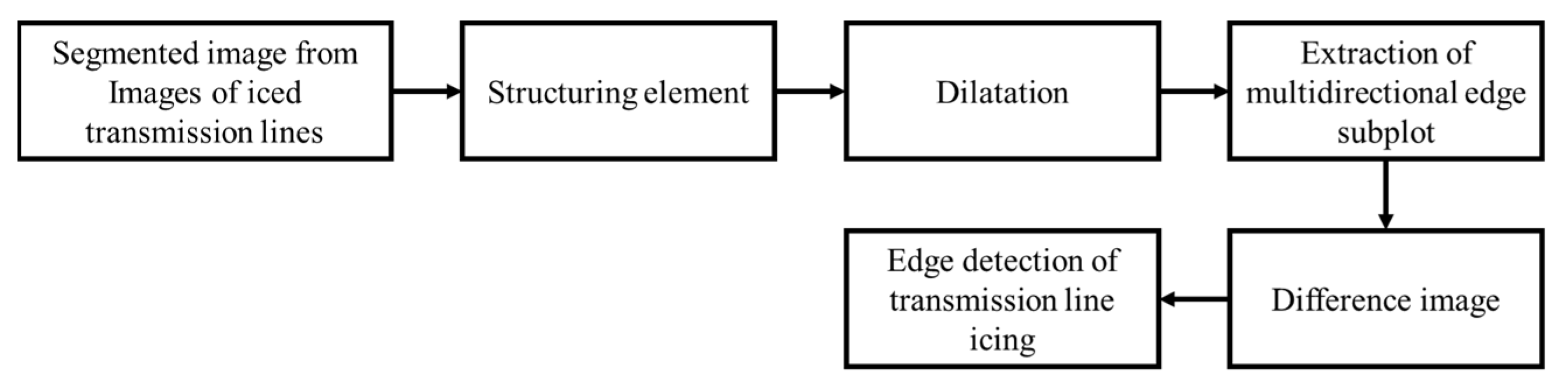
These morphological operations are performed on images based on shapes. They are structuring elements from it. It is a matrix containing '1' and '0' where '1' are called neighborhood pixels. The output pixel is determined by using these processing pixel neighbors. Here, the structuring element is used to dilate the image for edge extraction. The dilation operations are performed on images with different structuring elements. Dilation: Adding a pixel at an object boundary based on structuring elements. The rule for finding output pixels is the maximum input pixels in the neighborhood matrix.
3.7. Line Icing Identification
The next step is the identification of the line of the PTLI. At this stage, the upper and lower lines of the iced transmission line are determined for further analysis on 3D measurements. This study uses connected component labeling modification to distinguish between the upper and lower line. This method gives a unique label to each object in an image. Labeling each object by converting a binary image into a symbolic image, in which all pixels belonging to each connected component are uniquely labeled in this process. So the PTLI lines can be distinguished using unique labels (the top and bottom lines). In computer vision, connected component labeling detects connected regions in binary digital images.
The first scan assigns provisional labels to object pixels and records equivalences. Label equivalences are resolved during or after the initial scan. Then all equivalent labels on the second scan are replaced by representative labels. These two-scan labeling algorithms have some defects since a recursive algorithm possibly brings overflow. In addition, this method produced a good performance but took a long time. The implementation of image processing systems requires faster computer processing. Based on the above problems, this study modified the classic method for labeling connected components. This research on a one-time scanning algorithm with a scanning mask of size three is used so that the labeled pixels adjacent to the current object pixels will have the same label using the last-in-first-out stack processing scheme. The classic algorithm is enhanced by employing a larger scanning mask pattern to reduce the processing time and memory space required for analyzing neighboring pixels. The concept of scan mask technology to find 4-connectivity is presented in this subsection. The approach is that the image with the raster scanning direction is scanned from top to bottom, left to right, and pixel by pixel. The fundamental operation of each iteration is shown in Figure 11. In this method, the pixels will be mask scanned until an unlabeled object X pixel is found in the input image. Then, the object pixel X is labeled with the same label number as one of its neighboring pixels, P, Q, R, or S. In case of label conflicts, equality can be resolved by choosing the lower number, i.e..
Figure 11.
The scan mask with 4-connectivity (the current pixel X is compared to its neighbor's pixels P, Q, R, and S).
Figure 11.
The scan mask with 4-connectivity (the current pixel X is compared to its neighbor's pixels P, Q, R, and S).
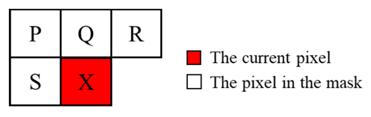
Figure 12 illustrates an example of the labeling used in this study. The labeling procedure utilized in this study is described below.
- Unlabeled object pixels with coordinates (0, 0) are shown in the scan mask represented by dotted lines.
- Based on point (b) in Figure 22, the label with '1' in the current pixel is processed.
- The mask is scanned at the next unlabeled pixel (2, 0).
- At point d, the labeling of pixels with '2' is illustrated. Currently, there are two labels on the pixel objects.
- The mask is scanned at the next unlabeled pixel (3, 0).
- Process of labeling with '2' again because its neighboring pixels are already labeled '2' so that expanded labeling area.
- The mask is scanned at the next unlabeled pixel (1, 1) in point (g).
- Pixels are labeled with '1' because the diagonals of adjacent pixels (0, 0) are already labeled with '1'.
- Because the pixels at location (1, 1) are labeled with '1', so expanded labeling area.
- The labeled areas '1' and '2' intersect, so the labeled area is expanded to a square of four pixels containing (0,0), (0,1), (1,0), and (1,1) using the expansion rule.
- The mask is scanned at the next unlabeled pixel (2, 1).
Figure 3.
An example of the labeling used in this research.

Labeled '1' because the left pixel has been labeled "1". Here, all eight connected neighboring pixels update their labels with minimum values.
4. Ice Thickness Calculation Using 3D Measurement
The principal indicator of an ice disaster is ice thickness. This section describes a method for ice thickness measurement based on our proposed iced transmission line identification scheme. Figure 13 illustrates the flowchart of the ice thickness calculation.
Figure 4.
The flowchart of ice thickness calculation.
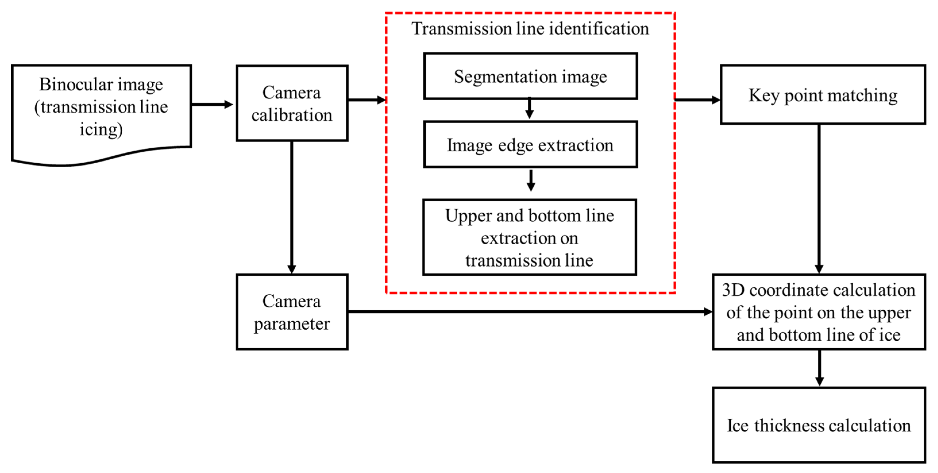
Given the binocular images, we first compute the camera parameters through camera calibration. Then, iced transmission line identification is used to find the top and bottom boundary of ice formed on power transmission lines. Next, the iced transmission line's 3D coordinates of the key points are computed using the key point matching method. Finally, the ice thickness is calculated.
The ice thickness is estimated after the 3D coordinate points are obtained. The 3D coordinate is graphing in more difficult than because depth perception is required. One can use projections onto the coordinate planes to simplify plotting points. The projection of a point onto is obtained by connecting the point to the by a line segment perpendicular to the plane and calculating the intersection of the segment of line with the plane. In this investigation, ice thickness was calculated using a three-dimensional Euclidean distance. Figure 14 shows a schematic diagram of 3D Euclidean distances.
Figure 5.
The diagram of 3D Euclidean distance.
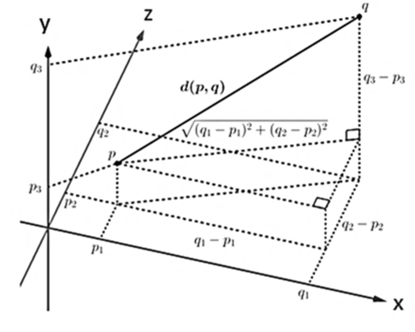
According to Figure 15, it will be calculated from the distance to in. Then the calculation formula is shown in formula number (24).
For example the distance between and is
Figure 6.
Illustration of ice thickness calculation in 3D measurement.
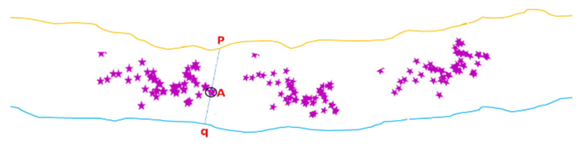
The three-dimensional calculation for ice thickness is adopted from the formula (24) above. Calculate the distance between the edge of the top line and the bottom line icing using the formula (25). After knowing the distance between both sides of the line icing, we subtract the distances from the diameter of the lines without icing (60mm) so that the ice thickness can be found. The formula for measuring ice thickness can be seen below.
With is the distance between the top and the bottom edge line, and is the diameter cable without ice load. Therefore, the ice thickness calculation in this research can be applied to measure line icing in straight or curved positions. Figure 15 shows an illustration of ice thickness calculation in 3D measurement. Based on Figure 15, to calculate the ice thickness in area A on the ice line, first, find the farthest point of the ice line in the upper and bottom boundary areas from point A to get points p and q. Point p is the farthest point from the upper line, and point q is the farthest from the bottom line. If we have the points of p and q, we can easily find the ice thickness using the formulas (24) and (25).
5. Experiment and Evaluation
On the PTLI dataset, we verify the effectiveness of our proposed method on the ice thickness measurement. Additionally, on the PTLI scene dataset, the overall performance of our method was evaluated using the confusion matrix. The segmentation results from the proposed method are compared with ground truth images. The proposed method aims to classify transmission line icing pixels on ROI as true positive, false negative, or false positive, as represented by accuracy, precision, and recall.
5.1. Dataset and Evaluation Matrix
5.1.1. Dataset
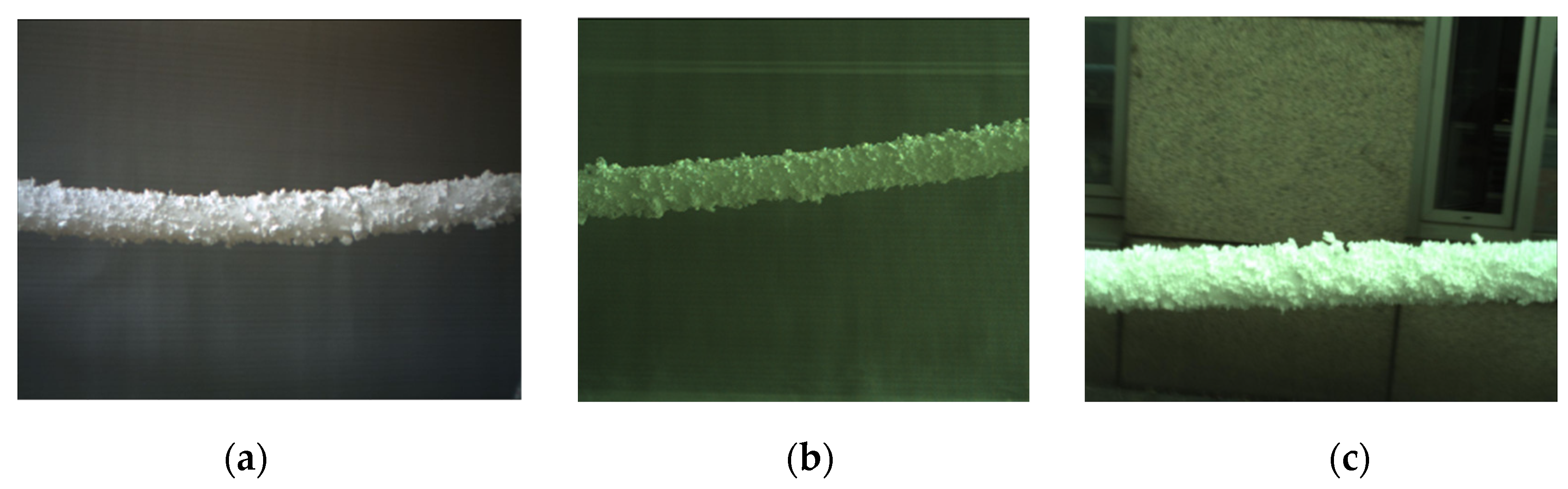
Our proposed method's iced transmission line identification performance is evaluated on the collected simulated PTLI scene dataset. A series of simulated PTLI scenes were independently generated to facilitate the collection of icing image data. Long cylindrical pearl cotton (Expandable Polyethylene, EPE) is used to simulate the transmission line, attached polystyrene foam (Expanded Polystyrene, EPS) is used to its surface as a simulated ice coating, and use pearl cotton as the background to simulate iced transmission line. So far, the iced transmission line scene is built and shown in Figure 16. The image pairs of the simulated PTLI dataset are collected via Daheng binocular camera. It is a huge and challenging work doing pixel-level labeling on collected images. Thus, the proposed method's measurement results of ice thickness are directly compared with the manual measurement results.
Figure 7.
Simulated ice scene images.
5.1.2. Evaluation Matrix
The segmentation results from our proposed scheme are compared with ground truth images which are segmented manually. The proposed scheme aims to classify transmission line icing pixels on ROI as true positive, false negative, or false positive, as represented by accuracy, precision, and recall. The system testing process is conducted using the confusion matrix. The confusion matrix can be interpreted as a tool that has a function to analyze whether the classifier is good at recognizing tuples from different classes. The values of True Positive (TP) and True-Negative (TN) provide information when the classifier in classifying data is true, while False Positive (FP) and False-Negative (FN) provide information when the classifier is incorrect in classifying data. Table 2 is the confusion matrix used to determine TP, TN, FP, and FN. After obtaining the TP, TN, FP, and FN values, accuracy, precision, recall, and specificity can be calculated using Equations (26-29).
Accuracy describes how accurate the model is in classifying correctly. The accuracy can be calculated using the formula in Equation (26).
Precision describes the accuracy between the requested data and the predicted results provided by the model. To calculate precision, use the formula in Equation (27).
Recall or sensitivity describes the success of the model in retrieving information. The formula in Equation (28) can be utilized to compute recall.
Specificity is used to measure the percentage of correctly identified negative data. To calculate specificity, use the formula in Equation (29).
5.2. Performance of The Proposed Method
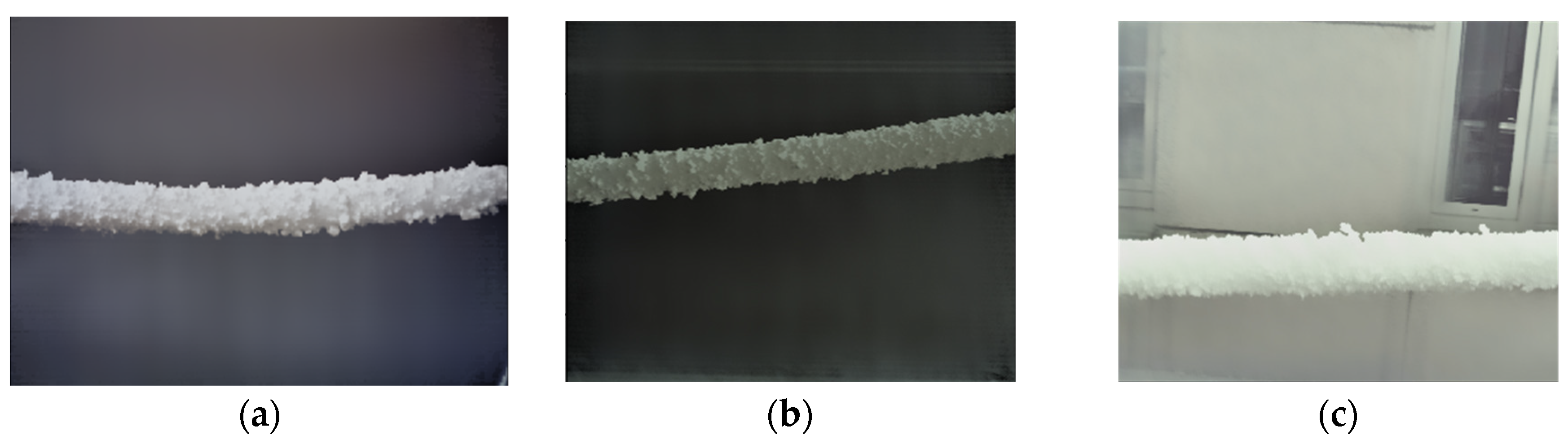
This section presents each stage of the experiment and evaluation results in our proposed scheme for identifying and extracting iced transmission lines. Three images with different illumination conditions and backgrounds are presented in this section as samples to test our proposed scheme. The three images are shown in Figure 17.
Figure 17.
Original image. (a) Image 1; (b) Image 2; (c) Image 3.
5.2.1. Image Color Restoration
At this stage, the image that appears dim and hazy, with a hue distorted from the original color, is corrected by preserving the original color. In general, this stage is used for color restoration; the lighting component in the image is removed. Figure 18 shows the image after color restoration using the method in this paper.
Figure 18.
The result of image color restoration. (a) Image 1; (b) Image 2; (c) Image 3.
Figure 18 shows that our method can restore image color while preserving the original color. The iced transmission line is brighter and more precise than the original image.
5.2.2. Image De-noising
In this stage, unwanted noise is removed and valuable information preserved, such as transmission line edges and transmission line icing textures. Figure 19 shows the image after the de-noising effect (filter noise).
Figure 19.
The image after the de-noising effect. (a) Image 1; (b) Image 2; (c) Image 3.
The proposed method in this paper for image de-noising has been successfully applied. Figure 19 shows that the image de-noising image is smoother, removes noise, and maintains the edges and texture of the transmission line icing.
5.2.3. Multilevel Threshold Segmentation
At this stage, the process separates the iced transmission line from a complex background containing objects and other noise. Pixels are generally grouped into various regions (objects and backgrounds) in this method. Figure 20 shows the results of the multi-threshold segmentation.
Figure 20.
The results of the multi-threshold segmentation. (a) Image 1; (b) Image 2; (c) Image 3.
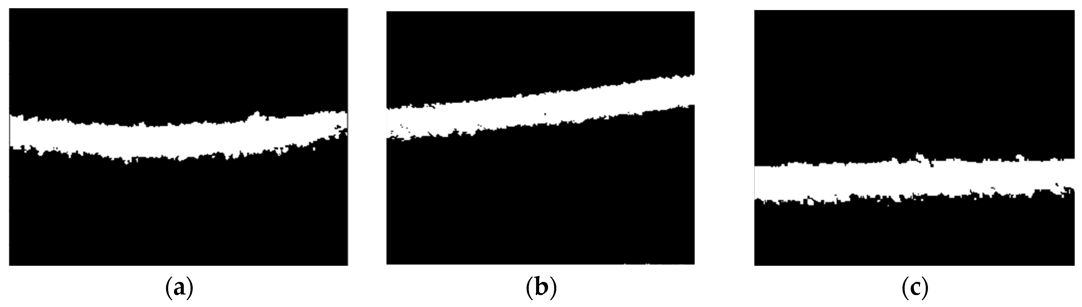
Figure 20 shows that our method successfully clusters pixels into different regions (object and background). After dividing several regions in the multi-threshold stage, the image successfully recognizes transmission line icing objects. At the same time, the background at this stage is eliminated.
5.2.4. Mathematical Morphology
Morphological operations are applied to segmented images to refine the segmented images. The gaps and holes are connected to neighboring objects and smooth objects. Figure 21 shows the result after the mathematical morphology operation.
Figure 21.
The result after mathematical morphology. (a) Image 1; (b) Image 2; (c) Image 3.
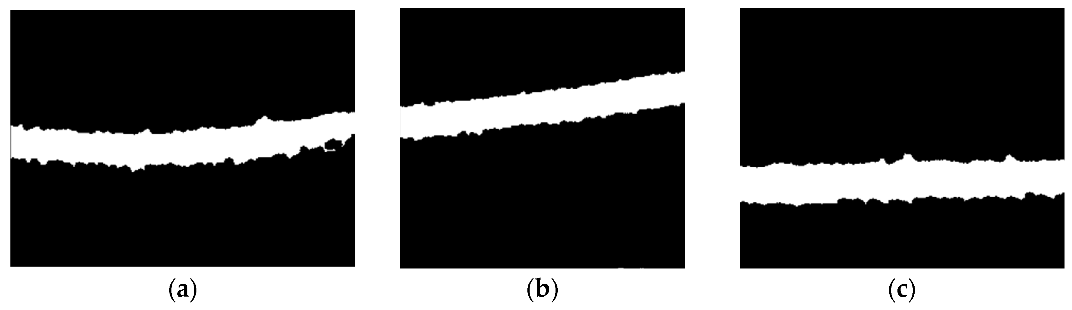
Based on Figure 21, morphological operations were successfully applied to segmented images. The image in the morphology operation is better because gaps and holes are connected to neighboring and smooth objects. The morphology image results will not change the image area or shape significantly.
5.2.5. Identifying Bounding Box
This stage consists of four stages. First, the image resulting from multi-threshold segmentation and morphology is changed again to an RGB image, selecting only the transmission line icing object and removing the background and foreground. Then the image is identified in the and parts of the object to determine the upper left and right, then lower left and right. Finally, the RGB image is selected on the ROI and returned to the binary image for further processing. Table 3 shows the process of selecting the region of interest.
5.2.6. Image Edge Extraction
The iced transmission line segmentation results were obtained by selecting the region of interest in the previous stage. Mathematical morphology is improved to expand the white area or emphasize the object's shape (transmission line icing). Determine the perimeter of objects within a binary image. If a pixel is non-zero, it is included in the perimeter and connected to at least one zero-valued pixel. Therefore, the edges of interior holes are considered part of the object's perimeter. Figure 22 shows the segmentation results and identifies the edges of the transmission line icing objects.
Figure 22.
The edges of the iced transmission line. (a) Image 1; (b) Image 2; (c) Image 3.
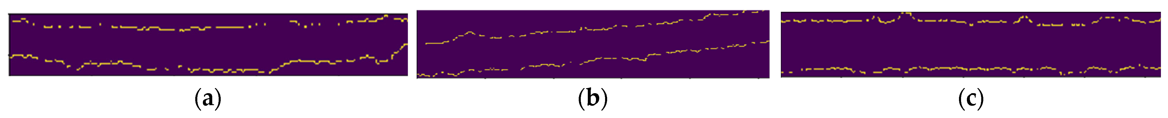
5.2.7. The Recognition of Transmission Line Icing
At this stage, the contours of the transmission line icing area are identified. The top and bottom lines of the iced transmission line were determined in advance for further analysis of the binocular vision scheme in 3D measurement. Thus, labeling is needed to recognize independent objects. This study connected component labeling is used to distinguish between upper and lower boundary areas or right and left. Figure 23 shows the edge-extracted images and images identified at the top and bottom of the line icing.
5.3. Verification and Analysis
Each image that becomes the test data will be marked with the edge of the iced transmission line by ground truth (expert labeling). System testing involves comparing the expert labeling results with our proposed scheme. By comparing the test image that an expert manually generated with the image that our proposed scheme detected, it is possible to determine the value of the Confusion Matrix component. The image will be converted into binary form. Then, the number of pixels detected by our proposed scheme will be known as the actual transmission line icing area by applying the AND operator. Transmission line icing will be marked with a binary value of 1, and non-line icing will be marked with a binary value of 0. Confusion Matrix validation is used in the performance testing of our proposed scheme. Figure 24 is an example of comparing ground truth detection results and our proposed scheme detection results.
The experiments in this paper were taken as test images from 50 images taken randomly. The Confusion matrix results from 50 PTLI images are shown in Table 4 based on the experiment.
Based on the result of the evaluation matrix for validation of our proposed scheme, the accuracy value is 97.71%, the precision value is 96.24%, the recall value is 86.22%, and the specificity value is 99.48%. Generally, our proposed scheme is reliable for PTLI images with complex backgrounds and images with poor lighting. Another advantage of this scheme is being able to distinguish between objects and backgrounds, making it easier to recognize objects in images with complex backgrounds. Identification of the top and bottom lines has also been successfully conducted by marking a different color between the top and bottom edges to make it easier to measure the thickness of the ice. Therefore, our proposed scheme effectively resolves iced transmission line identification issues and significantly increases automation.
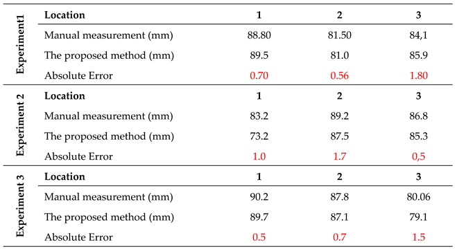
Our proposed scheme and manual measurement obtain the ice thickness values of specified locations from the three image pairs. In addition, the manual measurement results are measured by a micrometer caliper with an accuracy of 0.05 mm. Table 5 shows the comparison results in detail. It shows that the three image pairs are obtained by our method and manual measurement, respectively. It shows that the mean absolute error is small based on all experiments, so this scheme is acceptable for ice thickness measurement. Assume the actual value of ice thickness is the manually measured value; the average accuracy of our method can reach 90%.
6. Conclusions
This paper proposes a method of line icing identification for PTLI monitoring. In the initial stage, we integrate image restoration techniques with image filter enhancement to restore the image's color information. This combined approach effectively retains valuable information and preserves the original image quality, thereby mitigating noise introduced during the image acquisition. Subsequently, in the second stage, we introduced an enhanced multi-threshold algorithm to accurately separate background and target pixels. Through connected component labeling modification and mathematical morphology operations, we improve the image and get the region of interest (ROI) while eliminating the background regions. We apply the proposed method to measure ice thickness in the PTLI scene, and the average accuracy can be up to 90% compared with manual measurement. Based on the result of the evaluation matrix for validation of our proposed scheme, the accuracy value is 97.71%, the precision value is 96.24%, the recall value is 86.22%, and the specificity value is 99.48%. Our proposed scheme is reliable for PTLI images with complex backgrounds, images with poor illumination, and the position of the transmission cable object. Another advantage of this scheme is being able to distinguish between objects and backgrounds. Identification of the top and bottom lines has also been successfully conducted by marking a different color between the top and bottom lines to make it easier to measure the thickness of the ice. Therefore, this reliable scheme effectively resolves iced transmission line identification issues and significantly increases automation. Furthermore, we will apply the proposed method for Unmanned Aerial Vehicle (UAV) power line inspection and combine our method with correlation filters for other applications.
Author Contributions
The ideas and concepts were carried out in collaboration with all authors. N.R.N. and J.X. conceived and designed the experiments; N.R.N. and X.H. performed the experiments; N.R.N. and J.X. analyzed the data; N.R.N. and J.X. wrote the paper.
Conflicts of Interest
The authors declare no conflict of interest.
References
- Guo, Q. Research on the Key Technologies of Power Transmission Line Icing 3D Monitoring Based on Binocular Vision; 2018;
- Weng, B.; Gao, W.; Zheng, W.; Yang, G. Newly Designed Identifying Method for Ice Thickness on High-Voltage Transmission Lines via Machine Vision—High Volt. 2021. [Google Scholar] [CrossRef]
- Wang, J.; Wang, J.; Shao, J.; Li, J. Image Recognition of Icing Thickness on Power Transmission Lines Based on the Least Squares Hough Transform. Energies 2017. [Google Scholar] [CrossRef]
- Guo, Q.; Xiao, J.; Hu, X. New Keypoint Matching Method Using Local Convolutional Features for Power Transmission Line Icing Monitoring. Sensors (Switzerland) 2018. [Google Scholar] [CrossRef] [PubMed]
- Nusantika, N.R.; Xiao, J.; Hu, X. New Scheme of Image Matching for The Power Transmission Line Icing. In Proceedings of the ICIEA 2022 - Proceedings of the 17th IEEE Conference on Industrial Electronics and Applications; 2022. [CrossRef]
- Nusantika, N.R.; Hu, X.; Xiao, J. Improvement Canny Edge Detection for the UAV Icing Monitoring of Transmission Line Icing. In Proceedings of the 16th IEEE Conference on Industrial Electronics and Applications, ICIEA 2021; 2021. [CrossRef]
- Jiang, X.; Xiang, Z.; Zhang, Z.; Hu, J.; Hu, Q.; Shu, L. Predictive Model for Equivalent Ice Thickness Load on Overhead Transmission Lines Based on Measured Insulator String Deviations. IEEE Trans. Power Deliv. 2014. [Google Scholar] [CrossRef]
- Ma, G.M.; Li, C.R.; Quan, J.T.; Jiang, J.; Cheng, Y.C. A Fiber Bragg Grating Tension and Tilt Sensor Applied to Icing Monitoring on Overhead Transmission Lines. In Proceedings of the IEEE Transactions on Power Delivery; 2011. [CrossRef]
- Zarnani, A.; Musilek, P.; Shi, X.; Ke, X.; He, H.; Greiner, R. Learning to Predict Ice Accretion on Electric Power Lines. Eng. Appl. Artif. Intell. 2012. [Google Scholar] [CrossRef]
- Wachal, R.; Stoezel, J.S.; Peckover, M.; Godkin, D. A Computer Vision Early-Warning Ice Detection System for the Smart Grid. In Proceedings of the IEEE Power Engineering Society Transmission and Distribution Conference; 2012. [CrossRef]
- Lu, J.Z.; Zhang, H.X.; Fang, Z.; Li, B. Application of Self-Adaptive Segmental Threshold to Ice Thickness Identification. Gaodianya Jishu/High Volt. Eng. 2009. [Google Scholar]
- Gu, I.Y.H.; Berlijn, S.; Gutman, I.; Bollen, M.H.J. Practical Applications of Automatic Image Analysis for Overhead Lines. In Proceedings of the IET Conference Publications; 2013. [CrossRef]
- Hao, Y.; Liu, G.; Xue, Y.; Zhu, J.; Shi, Z.; Li, L. Wavelet Image Recognition of Ice Thickness on Transmission Lines. Gaodianya Jishu/High Volt. Eng. 2014. [Google Scholar] [CrossRef]
- Zhang, Y.; Wang, Y.; Wei, A. A New Image Detection Method of Transmission Line Icing Thickness. In Proceedings of the 2020 IEEE 4th Information Technology, Networking, Electronic and Automation Control Conference, ITNEC 2020; 2020. [CrossRef]
- Xin, G.; Jin, X.; Xiaoguang, H. On-Line Monitoring System of Transmission Line Icing Based on DSP. Proc. 2010 5th IEEE Conf. Ind. Electron. Appl. ICIEA 2010 2010, 186–190. [Google Scholar] [CrossRef]
- Lin Qi, Jing Wang, C.D.L. and W.L. Research on the Image Segmentation of Icing Line Based on NSCT and 2-D OSTU. Int. J. Comput. Appl. Technol. 2018, 57, 112–120. [CrossRef]
- Hemalatha, R.; Rasu, R.; Santhiyakumari, N.; Madheswaran, M. Comparative Analysis of Edge Detection Methods for 3D-Common Carotid Artery Image Using LabVIEW. In Proceedings of the Proc. IEEE Conference on Emerging Devices and Smart Systems, ICEDSS 2018; 2018. [CrossRef]
- Canny, J.F. A Computational Approach to Edge Detection. Pattern Analysis and Machine Intelligence. IEEE Trans. on, PAMI 1986. [Google Scholar] [CrossRef]
- Guo, Q.; Hu, X. Power Line Icing Monitoring Method Using Binocular Stereo Vision. In Proceedings of the 2017 12th IEEE Conference on Industrial Electronics and Applications, ICIEA 2017; 2018. [CrossRef]
- Liu, Y.; Tang, Z.; Xu, Y. Detection of Ice Thickness of High Voltage Transmission Line by Image Processing. In Proceedings of 2017 IEEE 2nd Advanced Information Technology, Electronic and Automation Control Conference, IAEAC 2017; 2017. [CrossRef]
- Gayathri Monicka, S.; Manimegalai, D.; Karthikeyan, M. Detection of Microcracks in Silicon Solar Cells Using Otsu-Canny Edge Detection Algorithm. Renew. Energy Focus 2022. [Google Scholar] [CrossRef]
- Lu, Y.; Duanmu, L.; Zhai, Z. (John); Wang, Z. Application and Improvement of Canny Edge-Detection Algorithm for Exterior Wall Hollowing Detection Using Infrared Thermal Images. Energy Build. 2022. [Google Scholar] [CrossRef]
- Zhang, Y.; Wang, Y.; Wei, A. A New Image Detection Method of Transmission Line Icing Thickness. Proc. 2020 IEEE 4th Inf. Technol. Networking, Electron. Autom. Control Conf. ITNEC 2020 2020, 2059–2064. [Google Scholar] [CrossRef]
- Jobson, D.J.; Rahman, Z.U.; Woodell, G.A. A Multiscale Retinex for Bridging the Gap between Color Images and the Human Observation of Scenes. IEEE Trans. Image Process. 1997. [Google Scholar] [CrossRef]
Figure 23.
Images after identified at the top and bottom of the line icing. (a) Image 1; (b) Image 2; (c) Image 3.
Figure 23.
Images after identified at the top and bottom of the line icing. (a) Image 1; (b) Image 2; (c) Image 3.
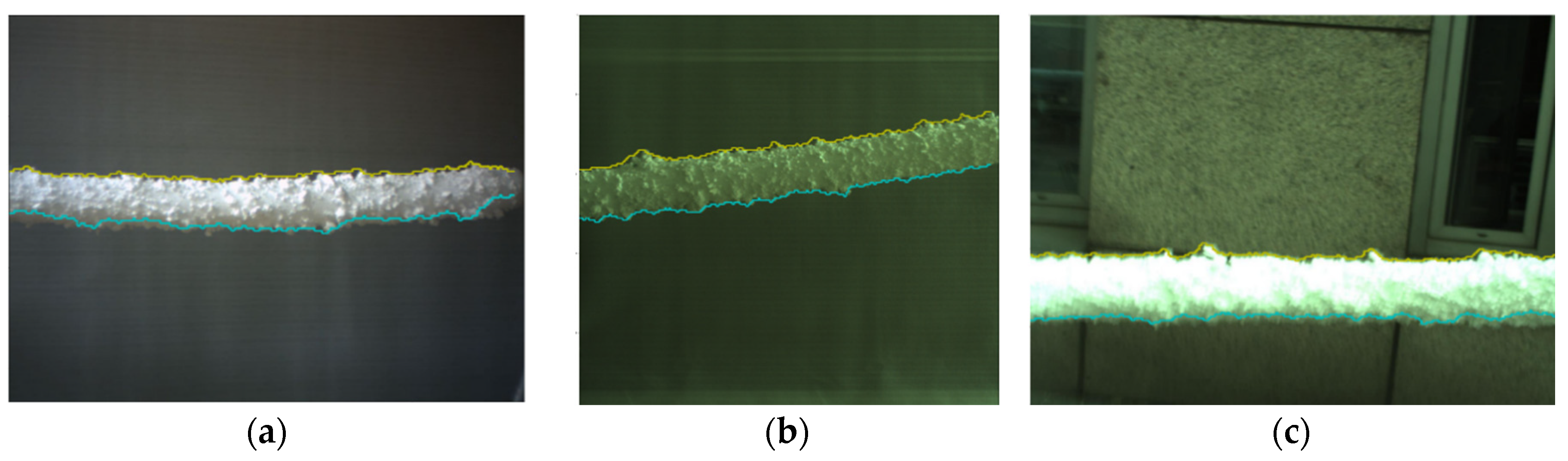
Figure 24.
Evaluation image. (a) Ground Truth Image Testing (b)The Proposed Method.
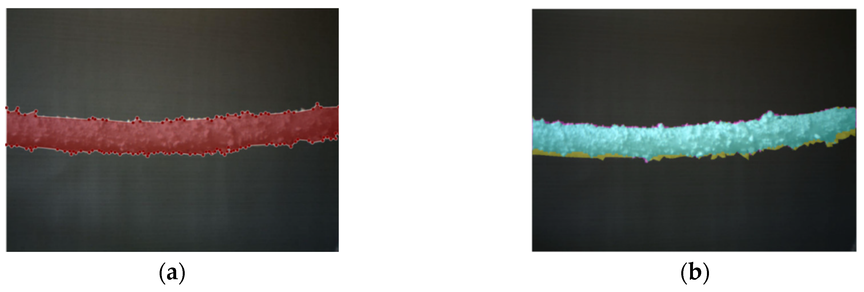

Table 1.
Image enhancement algorithm.
| Image enhancement algorithm |
|---|
| Data: input color image; the scales; the percentage of clipping pixels on each side |
|
Result: Image color restoration begin for each do //for each color channel for each do //for each scale // convolve the original image end // combining different scales with certain weights //color restoration simplest color balance end end |
Table 2.
Confusion matrix.
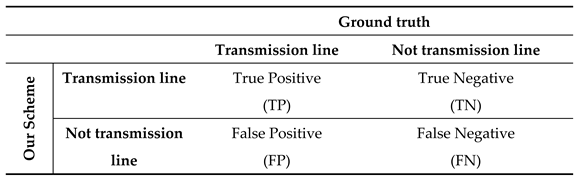 |
Table 3.
The Process of Selecting The Region of Interest.
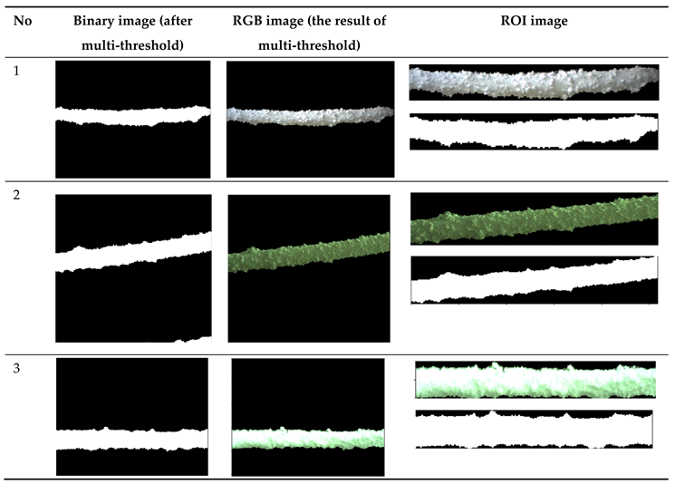 |
Table 4.
Confusion matrix from 50 PTLI images.
| Accuracy | Recall | Specificity | Precision |
| 0.9771 | 0.9624 | 0.8622 | 0.9948 |
Table 5.
The Experiment Result of Ice Thickness (mm).
 |
Disclaimer/Publisher’s Note: The statements, opinions and data contained in all publications are solely those of the individual author(s) and contributor(s) and not of MDPI and/or the editor(s). MDPI and/or the editor(s) disclaim responsibility for any injury to people or property resulting from any ideas, methods, instructions or products referred to in the content. |
© 2023 by the authors. Licensee MDPI, Basel, Switzerland. This article is an open access article distributed under the terms and conditions of the Creative Commons Attribution (CC BY) license (http://creativecommons.org/licenses/by/4.0/).
Copyright: This open access article is published under a Creative Commons CC BY 4.0 license, which permit the free download, distribution, and reuse, provided that the author and preprint are cited in any reuse.


