Submitted:
11 July 2023
Posted:
12 July 2023
You are already at the latest version
Abstract
The root system plays an irreplaceable role in plant growth. Its improvement can increase crop productivity. However, such system is still mysterious for us. The underlying mechanism has not been fully uncovered. The investigation on proteins related to the root system is an important means to complete this task. In the previous time, lack of root-related proteins makes it impossible to adopt machine learning methods for designing efficient models for the discovery of novel root-related proteins. Recently, a public database on root-related proteins was set up and machine learning methods can be applied in this field. In this study, we proposed a machine learning based model, named Graph-Root, for identification of root-related proteins. The features derived from protein sequences and one network were extracted, where the former features were processed by graph convolutional neural network and multi-head attention, and the later features abstracted the linkage between proteins. These features were fed into the fully connected layer to make prediction. The 5-fold cross-validation and independent tests suggested its good performance. It also outperformed the only one previous model, SVM-Root. Furthermore, the importance of each feature type and component in the proposed model was investigated.
Keywords:
Root-related proteins
; Deep learning
; Graph convolutional network
; Multi-head attention
; Network embedding
1. Introduction
The root system is a crucial component of plants. Root hairs in this system are tube-like extensions formed by some epidermal cells, which play important roles in plant growth and development. They increase the contact area between the root system and soil, facilitating the uptake of water and nutrients [1] and enhancing plant anchoring and interaction with microorganisms [2]. Root system architecture (RSA) refers to the spatial arrangement of roots in soil, which is an essential factor in plant growth and development [3]. Research on root and RSA is a hot area in plant biology [4] as it has important applications in agricultural production and ecological environments [5].
It is known that RSA is regulated by genes during growth and development [6]. The investigation on genes or proteins related to RSA is an important way to explore root traits. Discovering root-related genes can help us to understand root system, thereby designing proper scheme to enhance their resistance to stress and increase crop survival [7]. Such investigations are helpful to improve crop production with low input costs [4,8]. However, identification of genes or proteins related to root traits is challenging at present, which is still in an early stage [9].
In the past, research on RSA was less prevalent than above-ground studies. However, in recent years, with the development of gene identification techniques, work on root-related genes has been paid more attentions. The Arabidopsis root hairs have provided significant support in this regard [2]. Some techniques have been designed and used to identify root-related genes. Genome-wide association studies (GWAS) [10] have been utilized to identify genes associated with different plant root properties. For example, Xu et al. identified 27 genes related to root development of wheat using GWAS [11]. Kirschner et al. determined that ENHANCED GRAVITROPISM2 (EGT2) provided contributions to the root growth angle of wheat and barley [12]. Karnatam et al. screened out MQTLs associated with root traits through GWAS and discovered several root-related genes of maize [13]. Ma et al. adopted a similar scheme on the root system in wheat [14]. Fizames et al. identified a large number of Arabidopsis root-related genes using serial analysis of gene expression (SAGE) [15]. With the accumulation on root-related genes in these years, an online database, RGPDB [16], was set up recently, which collected root-related genes in maize, sorghum and soybean. It provided a strong data support for further investigating root-related genes.
In recent years, machine learning methods have wide applications in investigating gene and protein related problems. These methods always need lots of data. The root-related genes provided in RGPDB made it possible to investigate such genes using machine learning methods. In view of this, Kumar et al. developed an SVM-based root-related protein prediction method, named SVM-Root [17]. They extracted protein features from its sequence and employed several classic classification algorithms to build the model. To our knowledge, this was the first attempt to set up models for predicting root-related proteins using machine learning methods. Thus, the model has a great space for improvement. For example, this model adopted the protein sequence features, which cannot reflect all aspects of proteins.
In this study, a novel model, named Graph-Root, was proposed to identify root-related proteins in maize, sorghum and soybean. The validated root-related proteins (positive samples) were retrieved from RGPDB and other proteins under Viridi plantae were picked up as negative samples. Two types of features were extracted for each protein. The first type contained features extracted from protein sequences. Different from those used in SVM-Root [17], these features were derived from the raw features of amino acids, which can reflect the properties of proteins at amino acid level not at the sequence level. And the raw features were first refined by a graph convolutional network (GCN) [18] and then processed by a multi-head attention module [19] to access more powerful and unified features for protein sequences with different lengths. The second type reflected the linkage information between proteins, which were accessed by the well-known network embedding algorithm, Node2vec [20]. Features of two types were combined and fed into the fully connected layer (FCL) for making prediction. The cross-validation and independent tests suggested that Graph-Root had good performance and was superior to SVM-Root. The effectiveness of each feature type and all components in Graph-Root was also tested.
2. Materials and Methods
In this study, a binary classifier, named Graph-Root, was set up to identify root-related proteins. Several advanced computational methods were adopted. The entire procedures are illustrated in Figure 1. This section gave a description on the used materials and methods.
2.1. Dataset
Our study sourced the original information of root-related genes from RGPDB (http://sysbio.unl.edu/RGPDB/) [16], an online database containing more than 1200 candidate root-related genes, along with their corresponding promoter sequences. 576 genes for maize (zea maize), 355 for sorghum (sorghum bicolor), and 328 for soybean (glycine max) were obtained. To further access root-related proteins, we used gene IDs provided in RGPDB and searched for corresponding proteins in other publicly available databases. Specifically, root-related proteins for maize and soybean were retrieved from STRING (https://cn.string-db.org/, version 11.5) [21] and those for sorghum were obtained from Ensembl Genomes (https://www.ensemblgenomes.org) [22] by using its sub-module, EnsemblPlants. As a result, a total of 1259 root-related proteins were accessed. Furthermore, their sequences were also downloaded from above two databases. These protein sequences were termed as positive samples and we attempted to build a binary classification model for identifying root-related proteins.
When building binary classification models, negative samples are necessary. To this end, the reviewed proteins classified under Viridi plantae were extracted from the UniProt (https://www.uniprot.org/) [23], resulting in 41,538 protein sequences. These protein sequences and those of root-related proteins were combined to constitute the raw dataset. Then, this dataset was refined as follows: (1) protein sequences with length longer than 1000 were removed; (2) the well-known tool, CD-HIT [24] (cutoff = 0.4), was employed to remove homologous proteins. Accordingly, the result dataset contained 525 root-related proteins (positive samples) and 9260 other proteins (negative samples). The identity of any two proteins in such dataset was less than 0.4. To fully test the models, all positive and negative samples were equally and randomly divided into one training dataset (90%) and one test dataset (10%).
2.2. Protein Sequence Features
Protein sequence P is composed of several amino acids, which can be formulated by
where L is the length of the sequence. Features extracted from protein sequence are widely used to investigate protein-related problems. In this study, we also extracted protein features from its sequence. First, the raw features of amino acids were extracted. Then, these features were refined by a GCN module. Finally, to access informative protein features with unified size, a multi-head attention module was adopted.
2.2.1. Raw Features of Amino Acids
Two feature types of amino acids were used in this study. The first type was derived from the BLOSUM62 matrix [25], which is a substitution matrix. It is widely used in bioinformatics for scoring protein residues. Each component in this matrix indicates the correlation between two amino acids. By collecting such correlations on all 20 amino acids for one amino acid, a 20-dimension feature representation can be accessed for this amino acid.
The second feature type was obtained from position-specific scoring matrix (PSSM). This matrix reflects the frequency of amino acids at each position in a sequence alignment and also widely used to tackle various protein-related problems. Here, the PSI-BLAST [26] with Swissprot [27] database was used to generate the PSSM profiles for each protein sequence. It was performed with e-value of 0.001, 3 iterations, and default settings for other parameters. A 20-dimension feature representation was obtained for each amino acid in the protein sequences.
As mentioned above, each amino acid can be represented by 20 BLOSUM62 features and 20 PSSM features. For a protein sequence with length L, a ( in this study) feature matrix was constructed. Such matrix was denoted by X and would be refined in the following procedures. The distribution of raw features of amino acids is listed in Table 1.
2.2.2. Protein Contact Map Prediction
In above section, the raw feature representation of amino acids were obtained. Of course, the collection of these features for all amino acids in one protein sequence (i.e., X) can be used to represent the protein sequence. However, such representation was too ordinary, which can be refined by some advanced computational methods. This study selected GCN to refine these features. To execute GCN, a network with amino acids in the protein sequence as nodes must be constructed. We adopted SPOT-Contact-LM [28] to construct such network.
SPOT-Contact-LM is a neural network-based contact map prediction method that performs well in critical assessment of protein structure prediction experiments. This method utilizes the ESM-1b attention map as input features, integrates one-dimensional sequence features and one-hot encoding, and generates a contact map through the ResNet network. Given a protein sequence of length , SPOT-Contact-LM generates a contact probability matrix , where represents the probability that the -th amino acid contacts the -th amino acid. To extract reliable contacts between amino acids, the probabilities in the matrix were ranked from high to low and the top pairs of amino acids with highest probabilities were selected as the actual contacts. As the number of contacts in a protein is proportional to its length, was set to , where is a positive integer between 1 and 10. The original probability matrix is converted into an adjacent matrix , where if the i-th and j-th amino acids were the actual contacts; otherwise, it was set to zero. This adjacency matrix can indicate the structural features of the protein, which can be combined with raw features of amino acids to access more informative features of proteins.
2.2.3. GCN Module
For each protein sequence with length L, a feature matrix was constructed, which contained the BLOSUM62 and PSSM features of all amino acids in the sequence. On the other hand, an adjacent matrix was built using SPOT-Contact-LM, which indicated the contacts of amino acids in the sequence. GCN is a powerful tool, which can perfectly combine X and A, thereby generating a refined feature matrix for an input protein sequence. Generally, GCN contains several layers. Set as the input of the first layer of GCN and the output of the -th layer is denoted as . GCN updates using the following equation:
where is the sum of A and the identity matrix I (i.e., ), is the input feature matrix of the -th layer, denotes the weight matrix that can be trained, is the activation function, which was set to LeakyReLU. LeakyReLU has a fixed negative slope for negative values, making it more effective than the standard ReLU function. Prior to passing through the LeakyReLU activation function, each layer of the GCN module undergoes normalization to enhance the embedding effect. Finally, the output feature matrix, denoted by , is obtained, where represents the output dimension of each amino acid.
2.2.4. Multi-Head Attention Module
The output feature matrix was further refined by a multi-head attention module [19]. Its function included two aspects: (1) learn the importance of input features and focus on important features, and (2) make the feature dimension independent of protein length. The attention matrix can be produced using the following equation:
where and are the attention weight matrices. The Softmax function is used to normalize the feature vectors learned by the attention mechanism in different dimensions. We then multiply the learned attention matrix with the output of the GCN module as the final feature matrix of the protein derived from its sequence. As we selected FCL to make prediction, a flattening operation was performed on to obtain a feature vector of a fixed length for any protein sequence, i.e.,
2.3. Protein Network Features
The features derived from protein sequences can only reflect the properties of protein itself. Recently, the linkage of proteins were deemed as a different source for accessing protein features. Such features are always derived from one or multiple protein networks [29,30,31,32]. Here, we first constructed a protein network and then extract protein features from such network.
Given that proteins from multiple species were used in this study, we used the similarity of protein sequences to organize the network. In detail, BLASTP [26] was employed to compute the similarity between any two proteins. For protein p1 and p2, the similarity score yielded by BLASTP was denoted by . The protein network first defined all proteins under Viridi plantae as nodes. The edge was determined according to the similarity score between corresponding proteins. If the score was larger than zero, then the edge existed. After excluding isolated nodes (proteins), the final network contained 38,114 nodes and 4,353,907 edges. To express the different strengths of edges, each edge was assigned a weight, which was defined as the similarity score between corresponding proteins.
Above-constructed network contained abundant protein linkage information. The features derived from this network was helpful to identify protein functions. Several network embedding algorithms, such as DeepWalk [33], Mashup [34], and LINE [35], have been proposed, which can extract node embedding features from one or more networks. In this study, we adopted another well-known network embedding algorithm, Node2vec [20], to extract protein features from the network. This algorithm is an extended version of Word2vec [36], which can deal with network. Several paths are sampled from a given network in this algorithm following a predefined scheme. Then, the node sequence of each path is deemed as a sentence, whereas nodes are considered as words. This information is fed into Word2vec to extract node features.
This study used the Node2vec program sourced from https://github.com/aditya-grover/node2vec. It was applied on the constructed protein network with default parameters. The dimension of output features was set to 512. Accordingly, the protein network features were obtained, denoted by , where h=512.
2.4. Fully Connected Layer
Two feature types (sequence and network features) can be obtained for each protein in above procedures. Evidently, they reflected protein essential properties from different aspects. The combination of sequence and network features can contain more information of proteins, thereby improving the prediction quality. Thus, the sequence feature vector Y and network feature vector N were concatenated to comprise the final protein feature vector Φ, that is,
whereis the concatenation operation.
Subsequently, the final vector was fed into two FCLs with weight matrices and to make prediction. Finally, a Sigmoid function was employed to calculate the probability of an input protein being a root-related protein, which ranges from 0 to 1, formulated by
If the probability was higher than the threshold 0.5, the input protein was predicted to be root-related (positive); otherwise, it was predicted to non-root-related (negative).
2.5. Loss Function and Optimization
There were some parameters, such as in GCN module, and in multi-head attention module, and in two FCLs. These parameters can be optimized in terms of the loss function of binary cross entropy, which is defined as
where is the output of the model and y is the true label. The Adam optimizer [37] was deployed for optimizing above parameters.
2.6. Performance Evaluation
As previously mentioned, all investigated proteins were divided into one training dataset and one testing dataset. The training dataset contained 473 positive samples and 8,334 negative samples, whereas the testing dataset contained 52 positive samples and 926 negative samples. Clearly, the negative samples were much more than positive samples in the training dataset. The model based on such dataset may produce bias. Thus, we randomly sampled the same number of negative samples as the positive samples in the training dataset, resulting in a dataset with balanced size. On the balanced training dataset, we conducted 5-fold cross-validation to evaluate the performance of the model. As different negative samples may yield different predicted results, we conducted 50 repetitions of 5-fold cross-validation. In each repetition, the negative samples were resampled. The average performance under 50 rounds of 5-fold cross-validations was used to evaluate the model's performance. As for the test dataset, the model built on the training dataset was applied on it. Also, such test was executed 50 times with different negative samples in the training dataset. The average performance was picked up to assess the model’s performance on the test dataset.
For a binary classification problem, there exist many measurements to evaluate the performance of models. This study adopted the following measurements: sensitivity, specificity, accuracy, precision, F-score, Matthews correlation coefficient (MCC), and AUC [38,39,40]. To calculate these measurements, four entries should be counted in advance, including true positive (TP), false positive (FP), true negative (TN) and false negative (FN). Then, above measurements except AUC can be calculated by
Evidently, sensitivity measures the prediction accuracy of positive samples, whereas specificity measures the prediction accuracy of negative samples. Accuracy considers both types of samples. Precision represents the proportion of true positive predictions among all positive predictions, while F-score measures the balance between precision and recall (same as sensitivity). MCC provides a balanced assessment of the model's performance even if the sizes of classes are of great difference. These measurements evaluate the performance of models under a fixed threshold. AUC is different from them, which means the area under the receiver operating characteristic (ROC) curve. To draw this curve, several thresholds should be taken. Under each threshold, count the sensitivity and 1-specificity. After a group of sensitivity and 1-specificity are obtained, the ROC curve is plotted in a coordinate system with sensitivity as Y-axis and 1-specificity as X-axis. The area under such curve (i.e., AUC) is an important indicator to evaluate the performance of models. Generally, the larger the AUC, the higher the performance.
3. Results and Discussion
3.1. Hyperparameter Adjustment
There were several hypreparameters in Graph-Root. We tested several combinations of different hyperparameters and selected the optimal combination through the 50 rounds of 5-fold cross-validation.
From the output of SPOT-Contact-LM, we refined an adjacent matrix for each protein sequence. The hypreparameter is a key factor determining the number of contacts between amino acids. Several values between 1 and 10 were tried and we found that yielded the best performance.
In the GCN module, the number of GCN layers and their sizes were two key hypreparameters. For the number of layers, several studies have reported that if the number of GCN layers is too high, nodes will be embed too much neighbor information, leading to the overall feature becoming overly consistent and reducing the model's prediction ability. Generally, two layers are a proper setting, which was adopted in most studies. We also used a two-layer GCN module. For the layer sizes, a grid search was adopted to find out the best sizes. As a result, we found that the sizes were set to 256 for the former layer and 64 for the later layer can produce the best performance.
For the multi-head attention module, the number of attention heads was an important hypreparameter. It determined the contribution of each amino acid for reflecting the properties of proteins related to root. After experimental verification, we found that using 64 heads yielded good performance.
For the network features, the dimension was also a key hypreparameter, which determine how many informative features can participate in the construction of the model. If the dimension is too small, some key information cannot be included; whereas an excessively large dimension can lead to overfitting and low efficiency. Through validation, it was found that 512 was a proper choice and the model under this setting gave good performance.
Finally, for the two FCLs, the first layer was responsible for further fusing the features, while the second layer maps the feature dimension to the classification size. Our experimental results demonstrated that the size of the first FCL of 2048 effectively enhances the model's performance.
3.2. Performance of Graph-Root on the Training Dataset
The Graph-Root adopted the hyperparemeters mentioned in Section 3.1. On the training dataset, 5-five cross-validation was performed 50 rounds to evaluate the performance of Graph-Root. In each round, the negative samples were resampled, that is, negative samples were not same in each round. The average performance was counted to assess the final performance of Graph-Root. The measurements mentioned in Section 2.7 of Graph-Root are listed in Table 2. The accuracy, precision, sensitivity, specificity, F-score and MCC were 0.7578, 0.7411, 0.7958, 0.7197, 0.7668 and 0.5180, respectively. On the other hand, AUROC was 0.8130. Such results indicated good performance of Graph-Root.
3.3. Ablation Tests
There were several components in Graph-Root. To represent proteins, two types of features were constructed, including sequence features and network features, where sequence features further consisted of BLOSUM62 and PSSM features. On the other hand, there were several steps in Graph-Root, such as GCN module, multi-head attention module and FCL. To indicate that each feature type and step provided positive contributions for Graph-Root, several ablation tests were conducted.
For protein feature, the BLOSUM62, PSSM and network features were singled out one by one from the Graph-Root. The model without one of above feature types was also evaluated by 5-fold cross-validation. The prediction quality is provided in Table 3, including accuracy, precision, sensitivity, specificity, F-score and MCC. Furthermore, the ROC curves and their AUC values are illustrated in Figure 2. For easy comparisons, the performance of Graph-Root is also provided in Table 3 and Figure 2. From Table 3, we can see that when all feature types were used, the model (i.e., Graph-Root) provided best performance on all measurements except specificity, on which Graph-Root obtained the second place. As for AUC (Figure 2), Graph-Root also yielded the highest AUC. All these results suggested that all used features provided positive contributions to build the Graph-Root as the exclusion of each feature type reduced the performance of the model. However, their contributions were not same. It can be observed from Table 3 and Figure 2 that when BLOSUM62 feature was excluded, the performance of the model decreased most, followed by PSSM feature and network feature. It was implied that BLOSUM62 feature was relatively more important than PSSM and network features.
For the structure of Graph-Root, GCN and FCL were evidently important. To confirm this fact, we first remove GCN module from Graph-Root. In this model, BLOSUM62 and PSSM features were directly fed into the multi-head attention module. Such model was called Graph-Root without GCN. On the other hand, the FCL was also removed from Graph-Root. Different from Graph-Root without GCN, we only removed the first FCL as FCL was in charge of making prediction, that is, this model used a one FCL to make prediction. For convenience, such model was called Graph-Root without FCL. Above two models were also evaluated by 5-fold cross-validation. The evaluation results are available in Table 4 and Figure 3. Likewise, the performance of Graph-Root is also provided. Evidently, Graph-Root generally provided the best performance on almost all measurements, suggesting that GCN and FCL gave important contributions for improving the performance of Graph-Root. Furthermore, the removal of FCL gave a greater influence than the removal of GCN, implying FCL provided more contributions than GCN module.
3.4. Comparison with the Models Using Traditional Machine Learning Algorithms
The Graph-Root was constructed using some recently proposed machine learning methods, such as GCN and multi-head attention. As there were limited models for identifying root-related proteins using traditional machine learning algorithms, this section set up some models using such algorithms, thereby proving that the usage of new machine learning algorithms can improve the model.
We selected PSSM or network features to set up models. As PSSM matrix is of different sizes for proteins with different lengths, the PSSM Bigram method [41] was employed to process the original PSSM matrix for any protein. After such operation, the original PSSM matrix was converted into a matrix, thereby accessing a 400-dimension feature vector for any protein. Such obtained PSSM features or network features or the combination of PSSM and network features were fed into four widely used classic classification algorithms [42,43,44,45,46,47]: multilayer perceptron (MLP), decision tree (DT), support vector machine (SVM), random forest (RF), to set up the models. For convenience, we directly used the corresponding packages of these algorithms in scikit-learn [48]. The MLP had three hidden layers with sizes of 2048, 1024 and 256. The default setting was used for other parameters. All models were also evaluated by 5-fold cross-validation. The predicted results are listed in Table 5. For easy comparisons, the performance of Graph-Root is also listed in this table.
It can be observed from Table 5 that Graph-Root was better than other models despite which measurements were adopted. It was suggested that the employment of the deep learning techniques (GCN and multi-head attention) can really improve the model. Among the four classification algorithms, the model with MLP was generally better than other models, following by the model with RF; whereas the model with DT yielded the lowest performance. Furthermore, the models using network features were generally inferior to those using PSSM features. Such results were coincident with the results in ablation tests, that is, PSSM features were more important than network features.
3.5. Performance of Graph-Root on the Test Dataset
To fully test Graph-Root, an independent test was conducted on the test dataset. Such test was also performed 50 rounds with different negative samples in the training dataset. The predicted results were counted as accuracy of 0.7449, sensitivity of 0.7745, specificity of 0.7152 and AUC of 0.8225. Such performance was quite similar to the cross-validation results of Graph-Root on the training datasets, suggesting the good generalization of the Graph-Root.
3.6. Comparison with SVM-Root
To our knowledge, SVM-Root [17] is the only model for identifying root-related proteins. It adopted the protein features derived from its sequence and the classic classification algorithm, SVM, was adopted as the prediction engine. Its performance was also evaluated on the training dataset and further examined on a test dataset. The accuracy, sensitivity and specificity of SVM-Root on the training and datasets are illustrated in Figure 4. The performance, evaluated by same measurements, of Graph-Root is also shown in this figure. It can be observed that the accuracy and sensitivity of Graph-Root were clearly higher than those of SVM-Root, whereas the specificity of Graph-Root was slightly lower than that of SVM-Root. In general, Graph-Root was better than SVM-Root. Our model employed more essential information of proteins (sequence and network features) and adopted more efficient machine learning algorithms, which was the reason why our model was superior to SVM-Root.
4. Conclusions
In this study, we designed a machine learning based model for predicting root-related proteins in maize, sorghum and soybean. To access a full representation of each protein, several advanced machine learning methods were applied to protein sequences and network, thereby generating two feature types. This model was superior to the previous mode. All used features as well as the components in the model provided positive contributions for building the model. It is hopeful that this model can be a useful tool to identify novel root-related proteins and this study may attract more investigators' attention to investigate root-related problems in plants. The codes for Graph-Root are available at https://github.com/ken0414/Graph-Root.
Author Contributions
Conceptualization, L.C.; methodology, L.C. and S.L.; validation, L.C.; formal analysis, S.L.; data curation, L.C.; writing—original draft preparation, L.C. and S.L.; writing—review and editing, L.C.; supervision, L.C. All authors have read and agreed to the published version of the manuscript.
Funding
This research received no external funding.
Institutional Review Board Statement
Not applicable.
Informed Consent Statement
Not applicable.
Data Availability Statement
The data analyzed in this study are openly available in RGPDB (http://sysbio.unl.edu/RGPDB/), Uniprot (https://www.uniprot.org/), STRING (https://string-db.org/), and EnsemblPlants (https://plants.ensembl.org/index.html).
Conflicts of Interest
The authors declare no conflict of interest.
References
- Schiefelbein, J.W.; Somerville, C. Genetic control of root hair development in arabidopsis thaliana. Plant Cell 1990, 2, 235–243. [Google Scholar] [CrossRef]
- Grierson, C.; Nielsen, E.; Ketelaarc, T.; Schiefelbein, J. Root hairs. Arab. Book 2014, 12, e0172. [Google Scholar] [CrossRef]
- Ogura, T.; Goeschl, C.; Filiault, D.; Mirea, M.; Slovak, R.; Wolhrab, B.; Satbhai, S.B.; Busch, W. Root system depth in arabidopsis is shaped by exocyst70a3 via the dynamic modulation of auxin transport. Cell 2019, 178, 400–412. [Google Scholar] [CrossRef]
- Zhu, J.; Ingram, P.A.; Benfey, P.N.; Elich, T. From lab to field, new approaches to phenotyping root system architecture. Curr. Opin. Plant Biol. 2011, 14, 310–317. [Google Scholar] [CrossRef] [PubMed]
- Lynch, J. Root architecture and plant productivity. Plant Physiol. 1995, 109, 7–13. [Google Scholar] [CrossRef]
- Ober, E.S.; Alahmad, S.; Cockram, J.; Forestan, C.; Hickey, L.T.; Kant, J.; Maccaferri, M.; Marr, E.; Milner, M.; Pinto, F.; et al. Wheat root systems as a breeding target for climate resilience. TAG. Theor. Appl. Genetics. Theor. Angew. Genet. 2021, 134, 1645–1662. [Google Scholar] [CrossRef]
- Li, Y.; Liu, X.; Chen, R.; Tian, J.; Fan, Y.; Zhou, X. Genome-scale mining of root-preferential genes from maize and characterization of their promoter activity. BMC Plant Biol. 2019, 19, 584. [Google Scholar] [CrossRef] [PubMed]
- Jung, J.K.; McCouch, S. Getting to the roots of it: Genetic and hormonal control of root architecture. Front. Plant Sci. 2013, 4, 186. [Google Scholar] [CrossRef] [PubMed]
- Ramireddy, E.; Nelissen, H.; Leuendorf, J.E.; Van Lijsebettens, M.; Inzé, D.; Schmülling, T. Root engineering in maize by increasing cytokinin degradation causes enhanced root growth and leaf mineral enrichment. Plant Mol. Biol. 2021, 106, 555–567. [Google Scholar] [CrossRef]
- Bush, W.S.; Moore, J.H. Chapter 11: Genome-wide association studies. PLoS Comput. Biol. 2012, 8, e1002822. [Google Scholar] [CrossRef] [PubMed]
- Xu, F.; Chen, S.; Yang, X.; Zhou, S.; Wang, J.; Zhang, Z.; Huang, Y.; Song, M.; Zhang, J.; Zhan, K.; et al. Genome-wide association study on root traits under different growing environments in wheat (Triticum aestivum L.). Front. Genet. 2021, 12, 646712. [Google Scholar] [CrossRef]
- Kirschner, G.K.; Rosignoli, S.; Guo, L.; Vardanega, I.; Imani, J.; Altmüller, J.; Milner, S.G.; Balzano, R.; Nagel, K.A.; Pflugfelder, D.; et al. Enhanced gravitropism 2 encodes a sterile alpha motif-containing protein that controls root growth angle in barley and wheat. Proc. Natl. Acad. Sci. USA 2021, 118, e2101526118. [Google Scholar] [CrossRef]
- Karnatam, K.S.; Chhabra, G.; Saini, D.K.; Singh, R.; Kaur, G.; Praba, U.P.; Kumar, P.; Goyal, S.; Sharma, P.; Ranjan, R.; et al. Genome-wide meta-analysis of qtls associated with root traits and implications for maize breeding. Int. J. Mol. Sci. 2023, 24, 6135. [Google Scholar] [CrossRef]
- Ma, J.; Zhao, D.; Tang, X.; Yuan, M.; Zhang, D.; Xu, M.; Duan, Y.; Ren, H.; Zeng, Q.; Wu, J.; et al. Genome-wide association study on root system architecture and identification of candidate genes in wheat (Triticum aestivum L.). Int. J. Mol. Sci. 2022, 23, 1843. [Google Scholar] [CrossRef] [PubMed]
- Fizames, C.; Muños, S.; Cazettes, C.; Nacry, P.; Boucherez, J.; Gaymard, F.; Piquemal, D.; Delorme, V.; Commes, T.; Doumas, P.; et al. The arabidopsis root transcriptome by serial analysis of gene expression. Gene identification using the genome sequence. Plant Physiol. 2004, 134, 67–80. [Google Scholar] [CrossRef] [PubMed]
- Moisseyev, G.; Park, K.; Cui, A.; Freitas, D.; Rajagopal, D.; Konda, A.R.; Martin-Olenski, M.; McHam, M.; Liu, K.; Du, Q.; et al. Rgpdb: Database of root-associated genes and promoters in maize, soybean, and sorghum. Database J. Biol. Databases Curation 2020, 2020, baaa038. [Google Scholar] [CrossRef]
- Kumar Meher, P.; Hati, S.; Sahu, K.T.; Pradhan, U.; Gupta, A.; Rath, N.S. Svm-root: Identification of root-associated proteins in plants by employing the support vector machine with sequence-derived features. Curr. Bioinform. 2023, 18. [Google Scholar] [CrossRef]
- Kipf, T.N.; Welling, M. Semi-supervised classification with graph convolutional networks. ArXiv 2016, arXiv:1609.02907. [Google Scholar]
- Lin, Z.; Feng, M.; Santos, C.N.D.; Yu, M.; Xiang, B.; Zhou, B.; Bengio, Y. A structured self-attentive sentence embedding. arXiv 2017, arXiv:1703.03130. [Google Scholar]
- Grover, A.; Leskovec, J. Node2vec: Scalable feature learning for networks. In Proceedings of the 22nd ACM SIGKDD International Conference on Knowledge Discovery and Data Mining; ACM: San Francisco, CA, USA, 2016; pp. 855–864. [Google Scholar]
- Szklarczyk, D.; Kirsch, R.; Koutrouli, M.; Nastou, K.; Mehryary, F.; Hachilif, R.; Gable, A.L.; Fang, T.; Doncheva, N.T.; Pyysalo, S.; et al. The string database in 2023: Protein-protein association networks and functional enrichment analyses for any sequenced genome of interest. Nucleic Acids Res. 2023, 51, D638–D646. [Google Scholar] [CrossRef]
- Yates, A.D.; Allen, J.; Amode, R.M.; Azov, A.G.; Barba, M.; Becerra, A.; Bhai, J.; Campbell, L.I.; Carbajo Martinez, M.; Chakiachvili, M.; et al. Ensembl genomes 2022: An expanding genome resource for non-vertebrates. Nucleic Acids Res. 2022, 50, D996–D1003. [Google Scholar] [CrossRef]
- UniProt Consortium. Uniprot: The universal protein knowledgebase in 2023. Nucleic Acids Res. 2023, 51, D523–D531. [Google Scholar] [CrossRef]
- Fu, L.; Niu, B.; Zhu, Z.; Wu, S.; Li, W. Cd-hit: Accelerated for clustering the next-generation sequencing data. Bioinformatics 2012, 28, 3150–3152. [Google Scholar] [CrossRef]
- Henikoff, S.; Henikoff, J.G. Amino acid substitution matrices from protein blocks. Proc. Natl. Acad. Sci. USA 1992, 89, 10915–10919. [Google Scholar] [CrossRef]
- Altschul, S.F.; Madden, T.L.; Schaffer, A.A.; Zhang, J.H.; Zhang, Z.; Miller, W.; Lipman, D.J. Gapped blast and psi-blast: A new generation of protein database search programs. Nucleic Acids Res. 1997, 25, 3389–3402. [Google Scholar] [CrossRef]
- Boeckmann, B.; Bairoch, A.; Apweiler, R.; Blatter, M.C.; Estreicher, A.; Gasteiger, E.; Martin, M.J.; Michoud, K.; O’Donovan, C.; Phan, I.; et al. The swiss-prot protein knowledgebase and its supplement trembl in 2003. Nucleic Acids Res. 2003, 31, 365–370. [Google Scholar] [CrossRef]
- Singh, J.; Litfin, T.; Singh, J.; Paliwal, K.; Zhou, Y. Spot-contact-lm: Improving single-sequence-based prediction of protein contact map using a transformer language model. Bioinformatics 2022, 38, 1888–1894. [Google Scholar] [CrossRef]
- Pan, X.; Chen, L.; Liu, I.; Niu, Z.; Huang, T.; Cai, Y.D. Identifying protein subcellular locations with embeddings-based node2loc. IEEE/ACM Trans. Comput. Biol. Bioinform. 2022, 19, 666–675. [Google Scholar] [CrossRef]
- Zhang, X.; Chen, L.; Guo, Z.-H.; Liang, H. Identification of human membrane protein types by incorporating network embedding methods. IEEE Access 2019, 7, 140794–140805. [Google Scholar] [CrossRef]
- Pan, X.; Li, H.; Zeng, T.; Li, Z.; Chen, L.; Huang, T.; Cai, Y.-D. Identification of protein subcellular localization with network and functional embeddings. Front. Genet. 2021, 11, 626500. [Google Scholar] [CrossRef]
- Zhao, R.; Hu, B.; Chen, L.; Zhou, B. Identification of latent oncogenes with a network embedding method and random forest. BioMed Res. Int. 2020, 2020, 5160396. [Google Scholar] [CrossRef]
- Perozzi, B.; Al-Rfou, R.; Skiena, S. Deepwalk: Online Learning of Social Representations. In Proceedings of the 20th ACM SIGKDD International Conference on Knowledge Discovery and Data Mining, New York, NY, USA, 24–27 August 2014; pp. 701–710. [Google Scholar]
- Cho, H.; Berger, B.; Peng, J. Compact integration of multi-network topology for functional analysis of genes. Cell Syst. 2016, 3, 540–548. [Google Scholar] [CrossRef]
- Tang, J.; Qu, M.; Wang, M.; Zhang, M.; Yan, J.; Mei, Q. Line: Large-scale information network embedding. In Proceedings of the 24th International Conference on World Wide Web, Florence, Italy, 18–22 May 2015; pp. 1067–1077. [Google Scholar]
- Mikolov, T.; Chen, K.; Corrado, G.; Dean, J. Efficient estimation of word representations in vector space. In International Conference on Learning Representations; Scottsdale, AZ, USA, 2013. [Google Scholar]
- Kingma, D.P.; Ba, J. Adam: A method for stochastic optimization. In International Conference on Learning Representations; LA, USA, 2019. [Google Scholar]
- Powers, D. Evaluation: From precision, recall and f-measure to roc., informedness, markedness & correlation. J. Mach. Learn. Technol. 2011, 2, 37–63. [Google Scholar]
- Matthews, B. Comparison of the predicted and observed secondary structure of t4 phage lysozyme. Biochim. Biophys. Acta (BBA)-Protein Struct. 1975, 405, 442–451. [Google Scholar] [CrossRef]
- Chen, L.; Chen, K.; Zhou, B. Inferring drug-disease associations by a deep analysis on drug and disease networks. Math. Biosci. Eng. 2023, 20, 14136–14157. [Google Scholar] [CrossRef]
- Chowdhury, S.Y.; Shatabda, S.; Dehzangi, A. Idnaprot-es: Identification of DNA-binding proteins using evolutionary and structural features. Sci. Rep. 2017, 7, 14938. [Google Scholar] [CrossRef] [PubMed]
- Huang, F.; Fu, M.; Li, J.; Chen, L.; Feng, K.; Huang, T.; Cai, Y.-D. Analysis and prediction of protein stability based on interaction network, gene ontology, and kegg pathway enrichment scores. BBA—Proteins Proteom. 2023, 1871, 140889. [Google Scholar] [CrossRef]
- Huang, F.; Ma, Q.; Ren, J.; Li, J.; Wang, F.; Huang, T.; Cai, Y.-D. Identification of smoking associated transcriptome aberration in blood with machine learning methods. BioMed Res. Int. 2023, 2023, 5333361. [Google Scholar] [CrossRef]
- Ren, J.; Zhang, Y.; Guo, W.; Feng, K.; Yuan, Y.; Huang, T.; Cai, Y.-D. Identification of genes associated with the impairment of olfactory and gustatory functions in COVID-19 via machine-learning methods. Life 2023, 13, 798. [Google Scholar] [CrossRef]
- Wang, Y.; Xu, Y.; Yang, Z.; Liu, X.; Dai, Q. Using recursive feature selection with random forest to improve protein structural class prediction for low-similarity sequences. Comput. Math. Methods Med. 2021, 2021, 5529389. [Google Scholar] [CrossRef]
- Onesime, M.; Yang, Z.; Dai, Q. Genomic island prediction via chi-square test and random forest algorithm. Comput. Math. Methods Med. 2021, 2021, 9969751. [Google Scholar] [CrossRef] [PubMed]
- Wu, C.; Chen, L. A model with deep analysis on a large drug network for drug classification. Math. Biosci. Eng. 2023, 20, 383–401. [Google Scholar] [CrossRef] [PubMed]
- Pedregosa, F.; Varoquaux, G.; Gramfort, A.; Michel, V.; Thirion, B.; Grisel, O.; Blondel, M.; Prettenhofer, P.; Weiss, R.; Dubourg, V.J. Scikit-learn: Machine learning in python. JMLR 2011, 12, 2825–2830. [Google Scholar]
Figure 1.
The framework of Graph-Root. Protein features are derived from its sequence and a protein network. The sequence features are obtained from the raw features of amino acids that are further processed by graph convolutional network and multi-head attention modules, whereas the network features are extracted from a protein network via Node2vec. The sequence and network features are fed into fully connected layer to generate prediction.
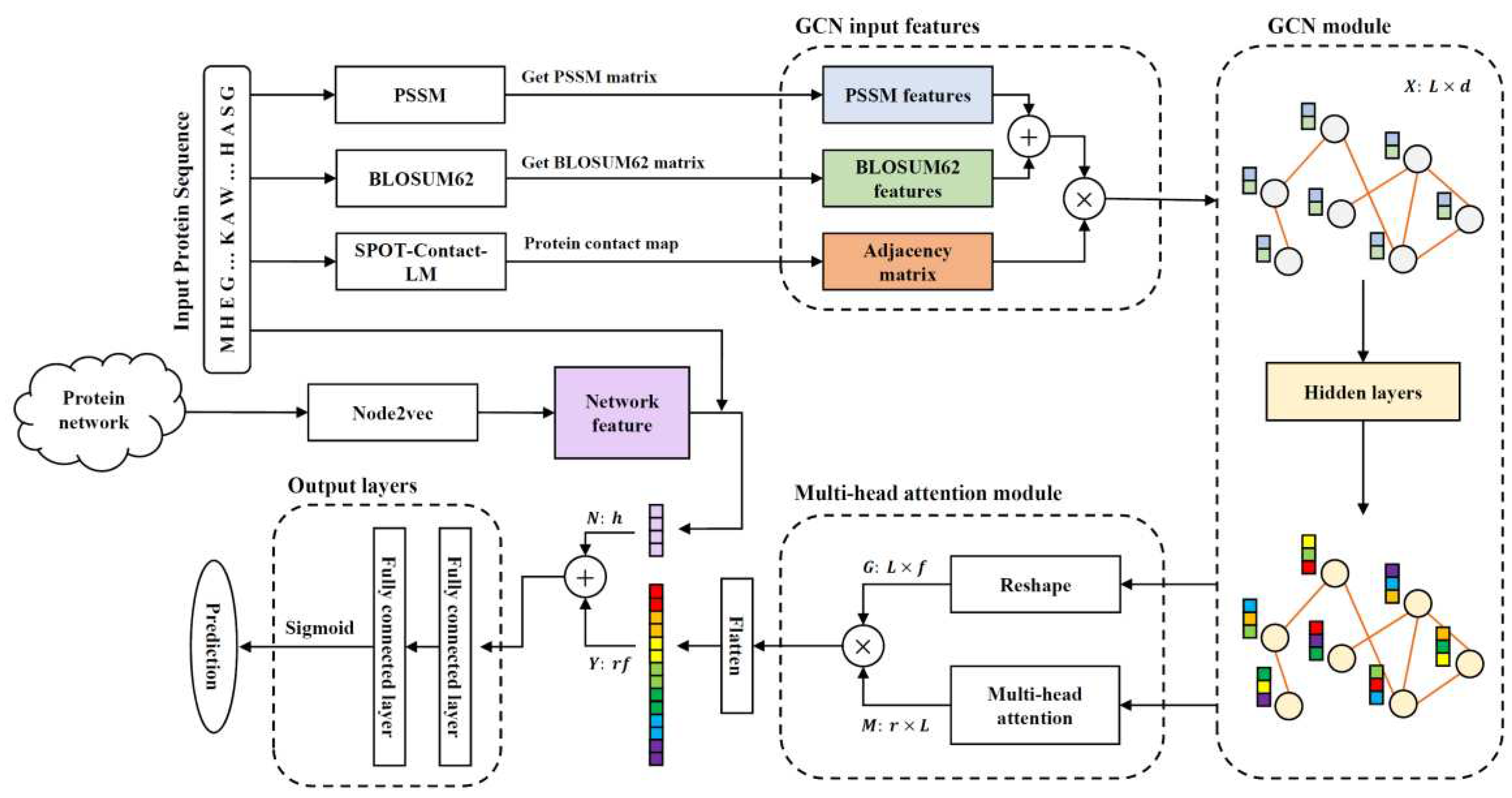
Figure 2.
ROC curves of Graph-Root and the model excluding one feature type. Evidently, when all features are used, the model (i.e., Graph-Root) yields the best performance.
Figure 2.
ROC curves of Graph-Root and the model excluding one feature type. Evidently, when all features are used, the model (i.e., Graph-Root) yields the best performance.
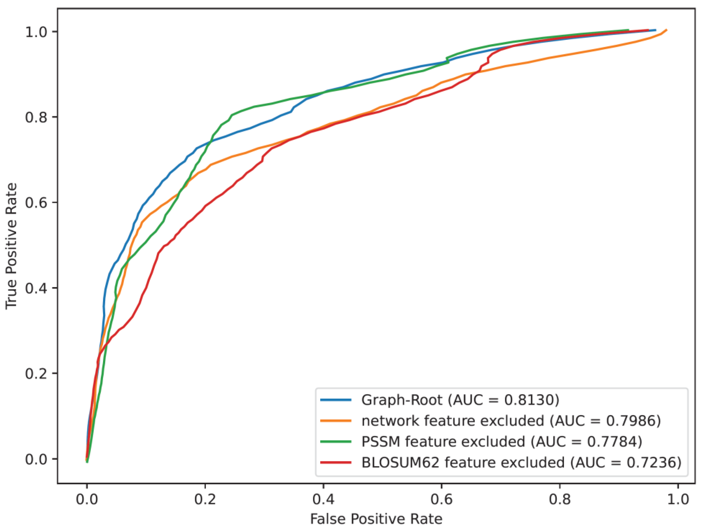
Figure 3.
ROC curves of Graph-Root and the models without GCN or FCL. Clearly, when GCN or FCL is removed, the model’s performance decreased.
Figure 3.
ROC curves of Graph-Root and the models without GCN or FCL. Clearly, when GCN or FCL is removed, the model’s performance decreased.
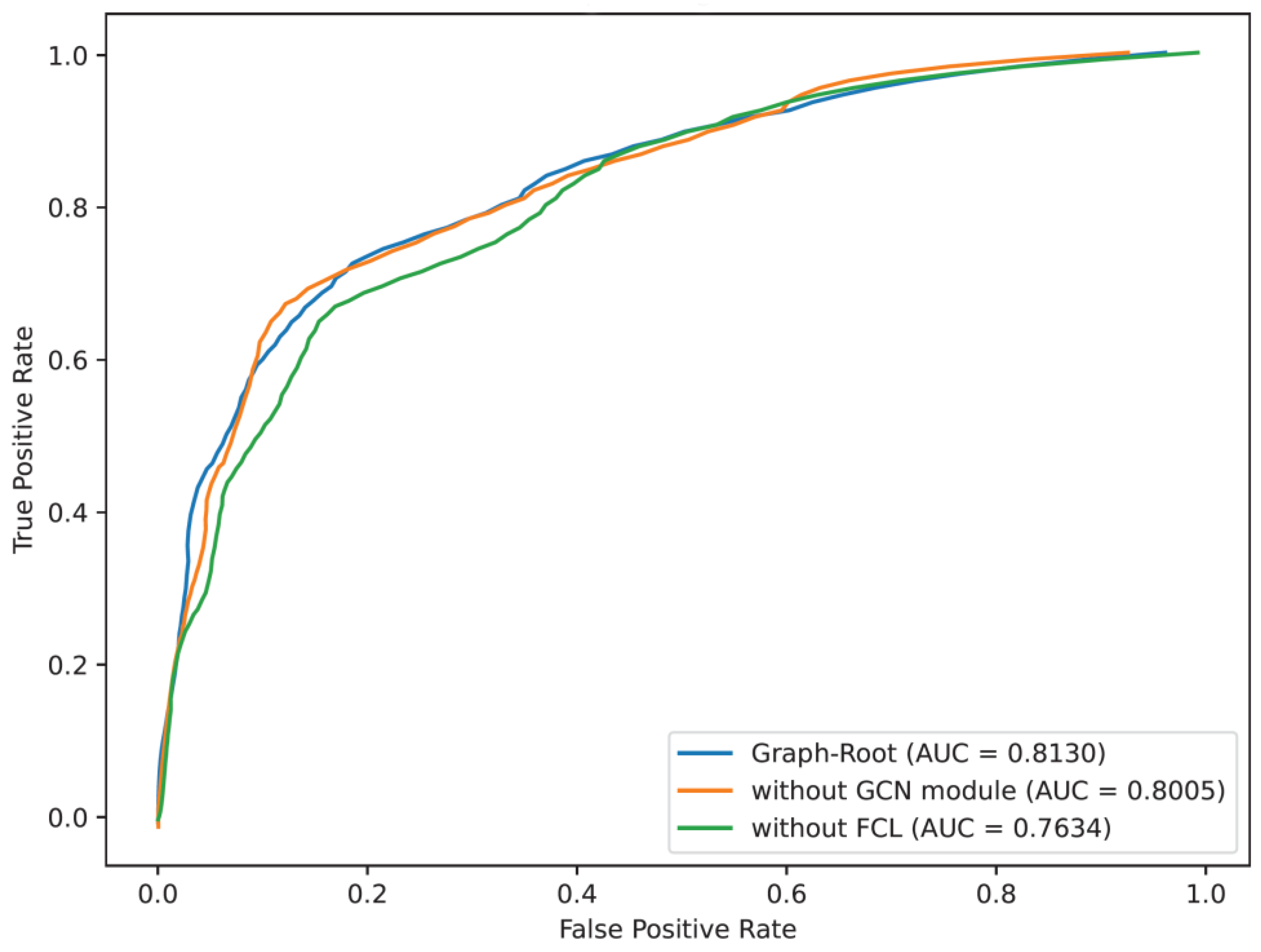
Figure 4.
A bar chart to compare Graph-Root and SVM-ROOT. Graph-Root generally outperforms SVM-Root.
Figure 4.
A bar chart to compare Graph-Root and SVM-ROOT. Graph-Root generally outperforms SVM-Root.
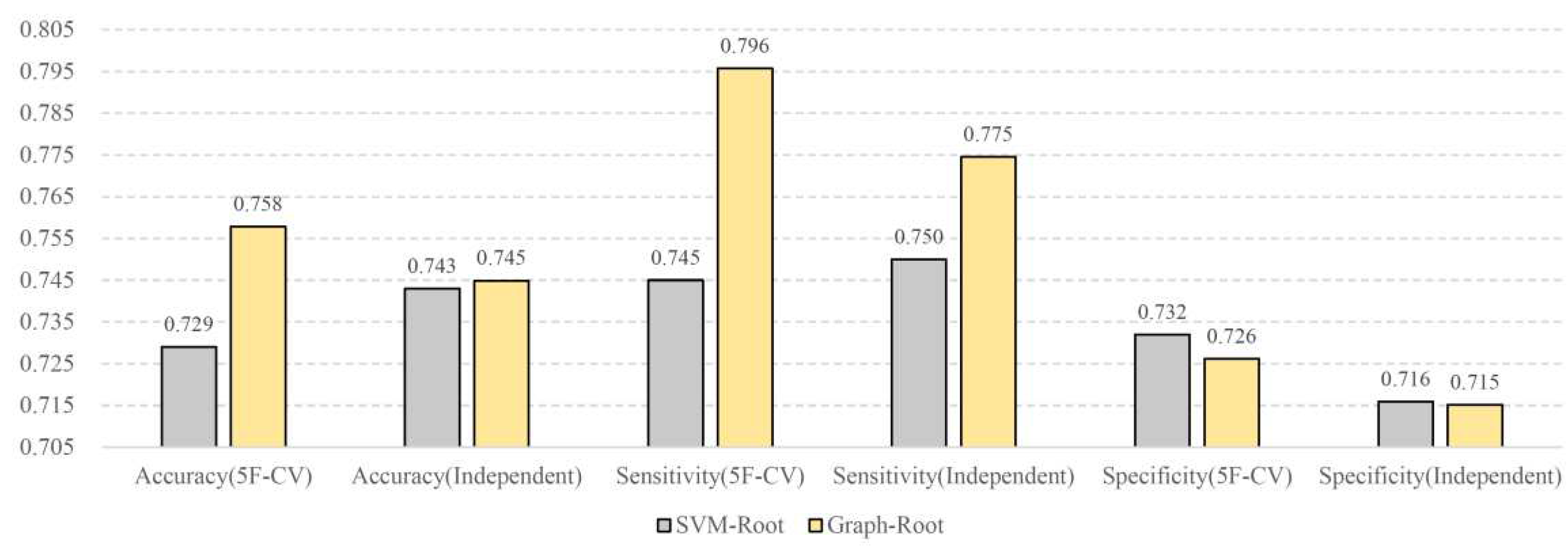

Table 1.
Two feature types of amino acids and their dimensions.
| Feature Type | Dimension |
|---|---|
| BLOSUM62 | 20 |
| PSSM | 20 |
Table 2.
Performance of Graph-Root on the training dataset under 50 rounds of 5-fold cross-validation.
Table 2.
Performance of Graph-Root on the training dataset under 50 rounds of 5-fold cross-validation.
| Measurement | Value |
|---|---|
| Accuracy | 0.7578 |
| Precision | 0.7411 |
| Sensitivity | 0.7958 |
| Specificity | 0.7197 |
| F-score | 0.7668 |
| MCC | 0.5180 |
| AUC | 0.8130 |
Table 3.
Results of ablation tests for features.
| Excluded feature | Accuracy | Precision | Sensitivity | Specificity | F-score | MCC |
|---|---|---|---|---|---|---|
| BLOSUM62 feature | 0.6743 | 0.6590 | 0.7272 | 0.6213 | 0.6906 | 0.3514 |
| PSSM feature | 0.7317 | 0.7239 | 0.7525 | 0.7108 | 0.7372 | 0.4647 |
| Network feature | 0.7489 | 0.7373 | 0.7768 | 0.7211 | 0.7558 | 0.4995 |
| No excluded feature(Graph-Root) | 0.7578 | 0.7411 | 0.7958 | 0.7197 | 0.7668 | 0.5180 |
Table 4.
Results of ablation tests for model architectures.
| Model | Accuracy | Precision | Sensitivity | Specificity | F-score | MCC |
|---|---|---|---|---|---|---|
| Graph-Root without fully connected layer | 0.7202 | 0.7246 | 0.7141 | 0.7262 | 0.7185 | 0.4414 |
| Graph-Root without GCN module | 0.7509 | 0.7382 | 0.7804 | 0.7213 | 0.7582 | 0.5033 |
| Graph-Root | 0.7578 | 0.7411 | 0.7958 | 0.7197 | 0.7668 | 0.5180 |
Table 5.
Comparisons of different models.
| Feature | Classification algorithm | Accuracy | Precision | Sensitivity | Specificity | F-score | MCC | AUC |
|---|---|---|---|---|---|---|---|---|
| PSSM feature | Multilayer perceptron | 0.7039 | 0.6940 | 0.7329 | 0.6747 | 0.7117 | 0.4098 | 0.7499 |
| Decision tree | 0.5828 | 0.5842 | 0.5804 | 0.5853 | 0.5813 | 0.1662 | 0.5829 | |
| Support vector machine | 0.6373 | 0.6432 | 0.6209 | 0.6535 | 0.6309 | 0.2754 | 0.6372 | |
| Random forest | 0.6609 | 0.6678 | 0.6437 | 0.6781 | 0.6546 | 0.3228 | 0.6609 | |
| Network feature | Multilayer perceptron | 0.6259 | 0.6196 | 0.6647 | 0.5869 | 0.6381 | 0.2554 | 0.6375 |
| Decision tree | 0.5479 | 0.5482 | 0.5482 | 0.5476 | 0.5473 | 0.0962 | 0.5479 | |
| Support vector machine | 0.5857 | 0.5761 | 0.6505 | 0.5207 | 0.6102 | 0.1734 | 0.5856 | |
| Random forest | 0.6173 | 0.6314 | 0.5685 | 0.6660 | 0.5975 | 0.2363 | 0.6173 | |
| PSSM and network feature | Multilayer perceptron | 0.7115 | 0.6965 | 0.7546 | 0.6684 | 0.7229 | 0.4265 | 0.7600 |
| Decision tree | 0.5786 | 0.5788 | 0.5802 | 0.5769 | 0.5788 | 0.1576 | 0.5786 | |
| Support vector machine | 0.6320 | 0.6343 | 0.6269 | 0.6370 | 0.6298 | 0.2645 | 0.6319 | |
| Random forest | 0.6684 | 0.6830 | 0.6322 | 0.7045 | 0.6558 | 0.3384 | 0.6684 | |
| Graph-Root | 0.7578 | 0.7411 | 0.7958 | 0.7197 | 0.7668 | 0.5180 | 0.8130 | |
Disclaimer/Publisher’s Note: The statements, opinions and data contained in all publications are solely those of the individual author(s) and contributor(s) and not of MDPI and/or the editor(s). MDPI and/or the editor(s) disclaim responsibility for any injury to people or property resulting from any ideas, methods, instructions or products referred to in the content. |
© 2023 by the authors. Licensee MDPI, Basel, Switzerland. This article is an open access article distributed under the terms and conditions of the Creative Commons Attribution (CC BY) license (http://creativecommons.org/licenses/by/4.0/).
Copyright: This open access article is published under a Creative Commons CC BY 4.0 license, which permit the free download, distribution, and reuse, provided that the author and preprint are cited in any reuse.


