
Submitted:
11 July 2023
Posted:
12 July 2023
You are already at the latest version
Abstract
This study investigated the mechanical properties and fatigue behavior of FH36 steel plate rolled in different directions. By adopting a sequential rolling process in the rolling direction (RD) and transverse direction (TD), the differences in properties between RD and TD were eliminated, resulting in nearly identical tensile properties. The steel plate exhibited a yield strength of approximately 420 MPa, a tensile strength of approximately 506 MPa, and an elongation of approximately 25%. Fatigue tests conducted at room temperature and -60℃ showed a fatigue limit of the maximum stress of 488 MPa at room temperature and 500 MPa at -60℃, indicating improved low-temperature fatigue performance. The fracture surfaces displayed distinct characteristics, such as oblique shearing fractures for high-cycle fatigue and cup-cone shape fractures for low-cycle fatigue. The fatigue source zone were both on the surface of the specimens. As the maximum stress increased, the area of the crack propagation zone for high-cycle fatigue decreased, while the area of the final fracture zone, the number of dimples and the proportion of the LAGBs increased.
Keywords:
ship plate steel
; tensile properties
; fatigue limit
; fracture observation
; texture
1. Introduction
In the field of shipbuilding and operation, ship plate steel was a crucial material that was subjected to various mechanical and environmental loads. Therefore, the study of the performance of ship plate steel was of utmost importance, especially in terms of tensile strength and fatigue properties.
Extensive and systematic research has been conducted on the tensile and fatigue performance of ship plate steel. Various grades of ship plate steel, such as A, D, E, and F grades had been studied. For example, Wang et al. [1,2] conducted a comprehensive study on the tensile and fatigue properties of EH36 ship plate steel in the temperature range of -60℃ to 20℃ They found that as the temperature decreased, the yield strength and ultimate tensile strength, resistance to low-temperature crack initiation and crack propagation of the steel plate all increased to varying degrees, but the plasticity decreased and the brittleness increased. As the stress ratio increased from 0.03 to 0.3, the fatigue crack propagation rate increased while the fatigue crack propagation threshold value decreased. In the research on different types of ship plate steel, differences in performance had been observed. Taking EH36 and FH36 ship plate steel as examples, Wang et al. [3] tested the fatigue crack propagation rates of EH36, DH36, and FH36 ship plate steels at room temperature, and found that EH36 steel had a higher fatigue crack propagation rate than the other steel due to its higher carbon content and smaller grain size.
Xu et al. [4] studied the fatigue crack growth process of AH36 steel and found that with the increase of stress amplitude and mean stress, the fatigue life of the steel significantly decreased. As the stress ratio increased, the CTOD (Crack Tip Opening Displacement) value gradually increased while the fatigue life decreased. Wang et al. [5] simulated the relationship curve between the stress intensity factor amplitude and the fatigue crack length of FH36 steel using ANSYS software, which was consistent with experimental results. They confirmed that the fracture mechanism of FH36 steel was microporous aggregation fracture and that it had large and deep dimples.
Regarding fatigue crack growth, some researchers had employed modified theoretical models for prediction. For instance, Le et al. [6] studied the fatigue crack propagation of AH36 steel by using the modified Irwin equation to calculate the plastic zone size at the crack tip in the residual stress range and the modified Wheeler model to predict the fatigue crack propagation process under various stress. The results showed that the theory of plastic zone size could describe the fatigue crack propagation behavior of the steel well, and the predicted results were in good agreement with the experimental data. Jiang et al. [7] studied the low-cycle fatigue behavior of shipbuilding steel 945. Through the cyclic stress-strain curve and the strain-life relationship, it was verified that the steel belongs to cyclic softening materials and had typical Masing behavior.
In addition to the aforementioned studies, new findings had emerged regarding fatigue failure. For example, it was generally believed that high-cycle fatigue failure of 65Mn steel components was caused by internal factors, while Li et al. [8] found that surface cracks can also lead to the high-cycle fatigue failure. Wang et al. [9] investigated the effect of two different specimen thicknesses on the fatigue crack propagation rate of shipbuilding steel through finite element simulation and experiments. They found that under the same maximum stress, the plastic zone at the crack tip of the thin specimen was significantly larger than that of the thick specimen, and the stress intensity factor at the crack tip was significantly greater than the theoretically calculated value.
In conclusion, there had been some research conducted both domestically and internationally on the fatigue crack propagation rate, fatigue life, and other aspects of ship plate steels such as FH36. However, there was a lack of research reports on the ambient and low-temperature cyclic fatigue behavior and mechanisms of ship plate steels, as well as the fatigue phenomena that occur when these steels were subjected to extreme conditions of high alternating stress. Therefore, in this study, FH36 steel was subjected to tensile performance tests, and based on these tests, ambient and low-temperature fatigue behavior of FH36 steel was investigated when it was subjected to maximum cyclic stresses exceeding the tensile strength. The aim was to understand the fatigue behavior and fatigue limits of the steel under extreme loading conditions. Furthermore, through fatigue fracture morphology and texture analysis and comparison, further study was conducted on the ambient and low-temperature fatigue behavior and differences. This research was expected to be beneficial for the safety design and assurance of ship plate steels under extreme loading conditions and for ensuring their service performance.
2. Materials and Methods
The FH36 ship plate steel was produced using a commercial controlled rolling and controlled cooling process. The chemical composition of the steel plate was shown in Table 1. The main process parameters were shown in Table 2, and the finished size was 54 mm × 3100 mm × 3100 mm.
According to the tensile testing standard GB/T 228.1-2010 [10], three specimens were taken along the RD and TD at 1/4 thickness position of FH36 steel plate (See Figure 1(a)), respectively. The dimensions of the tensile specimen were shown in Figure 1(b). Tensile tests were conducted on the above specimens using the SUNS universal testing machine with the tensile rate of 1 mm/min to obtain the stress-strain curves at room temperature. The specimen was cut 10 mm away from the fracture surface and polished with sandpaper. The ZEISS Sigma 500 field emission scanning electron microscope (SEM) and Bruker XFlash 6l 100 energy spectrometer were used to observe and analyze the fracture morphology and inclusion composition, respectively.
According to the fatigue testing standard GB/T 3075-2008 [11], specimens were taken along the RD of the steel plate and subjected to tension-tension fatigue tests at room temperature and -60℃. The specimens dimensions were shown in Figure 2. The stress ratio R was set to 0.1 and the number of cycles N was 107 for both room temperature and -60℃ low temperature tension-tension fatigue tests. The test specimens were considered to have completed the test when the number of cycles reached N or when they failed.
The fatigue limit test at room temperature of 25℃ was conducted by up and down method, in which the maximum cyclic stress of the first specimen was set to 500 MPa, and the stress increment Δσ was determined as 4% of the tensile strength. If the previous specimen didn't fail after N cycles or failed before completing N cycles, the stress of the next specimen was increased or decreased by Δσ accordingly. The frequency of the test was 150 Hz. The fatigue limits were determined at a low temperature of -60℃ by groups of conventional experimental method. The maximum cyclic stress applied were 480, 500, 520, 540, 560, and 590 MPa respectively, with a frequency of 120 Hz.
It was well known that the empirical formulas of S-N curve included power function Basquin model, exponential function model, three-parameter model, etc [12,13]. The Basquin model was only suitable for medium to low fatigue life, while the three-parameter model was suitable for fitting S-N curves in the low fatigue life zone and also had application value in fitting S-N curves in the medium and high fatigue life zone and the overall fitting effect was good [14,15]. Therefore, we used the three-parameter model to fit the S-N curve during the low-temperature fatigue test. The parameters in this model were commonly determined using the least squares method by researchers. For instance, Little et al. [16] used linear regression to fit the logarithmic mean S-N curve of the life samples and solve the parameters. Ling et al. [17] estimated the parameters in the model using maximum likelihood and moment methods. Zheng et al. [18] employed the direct modeling method of GM(1,1) in grey system theory to determine the three parameters in the model. Xie et al. [19] fitted the experimental data using a double-weighted least squares method. Gao et al. [20] used the linear correlation coefficient as the objective function and determined the parameters through BASIC programming, which resulted in a better fit of the S-N curve experimental data. Therefore, in this study, the method proposed by Gao et al. was adopted, and the relevant parameters were determined using MATLAB programming.
After the fatigue test, the fracture surface was cut 10 mm away from the fracture position of the fatigue specimen, ground flat using sandpaper, and then observed using the SEM. The energy spectrometer was used to determine the composition of the fracture inclusions. In addition, wire cutting was used to cut 10 mm length along the tensile direction from the fracture surface of fracture specimens and the center of the unfractured specimens at room temperature, and 2 mm thickness perpendicular to the tensile direction was cut to obtain the fatigue section specimens. The sections of the specimens parallel to perpendicular to the tensile direction were mechanically polished with sandpaper, and then vibration polishing was used to remove the stress layer. The morphology of the above sections was observed using the SEM. The grain boundaries and texture for the sections was analyzed by using the SEM equipped with an Oxford SYMMETRY EBSD detector and the Aztec Crystal software.
3. Results and discussion
3.1. Analysis of tensile properties test results and morphological observation
3.1.1. Analysis of tensile properties test results
Figure 3 showed the stress-strain curves of FH36 steel plate along the rolling direction and transverse direction at 1/4 thickness. From the figure, it can be seen that the repeatability of the curves was good, and the positions of the curves for the two types of specimens were relatively close. Figure 4 showed the strength and plasticity data of the two types of specimens calculated from Figure 3. It can be seen from the figure that the mechanical performance data of FH36 steel plate at 1/4 thickness in the RD and TD both met the performance requirements of the standard GB/T 712-2011 [21], and the data of the RD and TD were quite close. The yield strength in the RD was slightly lower than that in the TD, but the toughness was slightly higher than that in the TD, and the difference between the two was very small. This may be related to the fact that the steel plate was first rolled in the RD and then in the TD, and the deformation amount in the RD and TD was basically the same, which eliminated the performance difference between the RD and TD.
3.1.2. Tensile test fracture surface observation
Figure 5 showed the tensile fracture macroscopic morphology (a, d), fiber zone morphology (b, e), and shear lip morphology (c, f) of the FH36 steel plate at 1/4 thickness. From Figure 5(a) and (b), it can be seen that the tensile fracture surface was cup and cone-shaped, with the center of the fracture being a rougher fiber zone and the edges being a smoother shear lip zone. No obvious radical zone was observed, indicating that the deformation constraint was small and the plasticity was good [22,23]. The shear lips were oriented at a 45° angle to the main stress. The proportion of the fiber zone of the specimen in the RD was larger than that in the TD, indicating better plasticity in the RD, which was consistent with the plasticity results in Figure 4. The shear lips in the TD had less symmetric, smooth and complete compared to the RD [24].
From Figure 5(b) and (e), it can be seen that there were both equiaxed dimples (Deq) and spherical inclusions in the fibrous area of the fracture surfaces in the RD and TD. Usually, large dimples were nucleated by inclusions, while small dimples were nucleated by carbides. Compared to Figure 5(b), there were more large dimples in Figure 5(e), indicating a higher content of inclusions and lower plasticity and toughness of the specimen [25]. There was a large-sized spherical inclusion with a diameter up to 20 um in Figure 5(b).
Table 3 presented the energy spectrum analysis results for the inclusion at the location indicated by the red cross. Based on the elemental content ratios, it can be inferred that the inclusion was a composite inclusion consisting primarily of Al2O3-CaO, with small amounts of CaS, TiC, SiC, NbC, Ni7C3, MnS, and other compounds [26,27,28]. Generally speaking, oxide inclusions that existed in the molten steel can act as nucleation sites for the precipitation of sulfides and other compounds. Therefore, it was common to find oxide inclusions enveloped by a layer of sulfide inclusions and other constituents in steel, forming composite inclusions [29].
3.2. Fatigue test results and analysis at room temperature
3.2.1. Fatigue test results at room temperature
The results of the room temperature fatigue tests for the steel plate were shown in Table 4.
The fatigue limit was calculated by using the following formula based on the above data:
WherWhere, m was the total number of valid test cycles, R was the stress ratio, σi was the maximum stress for the i-th level, and Vi was the number of valid cycles at the maximum stress for the i-th level.
The fatigue limit σ-1(107) calculated from the formula was 488 MPa. The specimen didn't fail under the maximum stress of 460 MPa, while it failed under the maximum stress of 480 MPa and 500 MPa, but with a cycle number greater than 105 for both. However, when the maximum stress was 520 MPa, the specimen failed with a cycle number less than 105. Therefore, it can be inferred that high-cycle fatigue occurred at the maximum stress of 500 MPa and below, while low-cycle fatigue occurred at 520 MPa and above, as shown in Table 5. Figure 6 showed the up-and-down diagram constructed based on the test results.
3.2.2. Fatigue test fracture morphology observation and analysis
Figure 7 showed the macroscopic morphology of the fatigue fracture surface of failed specimens under different maximum stress as listed in Table 4. From Figure 7(a) and (b), it can be observed that there was no significant plastic deformation near the fracture under the maximum stress of 480 MPa and 500 MPa, and the fracture was a oblique shear fracture. The fracture showed a static fracture zone caused by crack propagation, indicating good plasticity [30]. From Figure 7(c), it can be seen that due to the maximum stress of 520 MPa being greater than the material's tensile strength, there was significant macroscopic plastic deformation near the fracture surface. As a result, the effective cross-sectional area decreased, and an overload fracture occurred, resulting in a cup-and-cone-shaped fracture with good ductility, similar to the fracture surface of a tensile specimen [31].
Fatigue fracture surfaces typically consisted of three zones: the flat and shiny fatigue source zone (I zone), the fatigue crack propagation zone (II zone) with fan-shaped fatigue striations, and the rough fatigue final fracture zone (III zone), as shown in Figure 8. The size of the II zone was related to the fatigue critical crack length ac, and when the crack length reached ac, the specimen began to undergo rapid fracture [32].
Figure 9 showed the fatigue fracture surface of specimens RT6, RT8, and RT12 under the maximum stress of 480 MPa from the Table 4. It can be seen from the figure that all the fracture surface consisted of the I, II and III zones. From Figure 9(a), (d) and (g), it can be observed that the I zone was located at the surface of the specimens. This was because under cyclic loading, the highest stress in the specimen was applied on the surface. The defects such as slip bands, grain boundaries, and inclusions, which existed in the surface, would develop into severe stress concentration positions. Fatigue fracture was very sensitive to the positions, thus micro-cracks first formed in the surface [33,34]. Meanwhile, the surface where the fatigue crack initiated was relatively smooth, therefore the fracture surface showed a single fatigue source. According to Figure 8, the estimated ac values for the II zone of the RT6, RT8, and RT12 specimens in Figure 9 were 2.0 mm, 2.3 mm, and 2.3 mm, respectively. The average ac value was approximately 2.2 mm. The characteristic of the fatigue striations in the II zone was that the width increased as the distance from the I zone increased [35]. In addition, there were also significant fatigue steps in this zone, which were formed by the intersection of different fracture surfaces, and the direction of the striations was generally consistent with the normal direction of the fatigue striations [36]. For the III zone, under tension-tension fatigue test conditions, the dimples were almost circular and equiaxed, and there were spherical and irregular cotton-like inclusions near the dimples (see Figure 9(c), (f), (i)).
Figure 10 showed the fatigue fracture morphology of specimen RT5 under the maximum stress of 500 MPa as listed in Table 4. From Figure 10(a), it can be seen that the I zone was located at the surface. As the maximum stress was higher than 480 MPa, the ac was about 1.9 mm, significantly lower than the 2.2 mm under the maximum stress of 480 MPa. Therefore, the range of the II zone was smaller, the range of the III zone was larger, and the fatigue striations were finer and less obvious [37]. From Figure 10(b), it can be seen that the II zone was mainly characterized by cleavage fracture with a river-like pattern. From Figure 10(c), it can be observed that there were more dimples in the III zone compared to that under the maximum stress of 480 MPa, and the diameter of the larger dimples was also larger.
Figure 11 showed the fatigue fracture morphology of specimens RT2 and RT4 from Table 4 under the maximum stress of 520 MPa. As shown in Figure 11(a) and (d), it can be seen that the cross-sectional area near the fracture was much smaller due to significant plastic deformation (as shown in Figure 7(c)) than that under the low maximum stress (as shown in Figure 10(a)). The microstructure of the fracture surface was similar to that of the tensile fracture, with a fiber zone and a shear lip zone, but no clear I and II zone. From Figure 11(b), it can be seen that the elongated dimple (Del) appeared in the shear lip zone of the edge. From Figure 10(e), it can be seen that there were circular fatigue striations in the shear lip zone, with river-like patterns, as well as irregular inclusions. From Figure 11(c) and (f), it can be seen that there were many Deq in the fiber zone, but the size of the large dimples (as seen in Figure 11(c)) was not as large as that under 500 MPa (see in Figure 10(c)). There were cotton-like and spherical inclusions of various sizes inside the dimples (see in Figure 11(c)) and (f)).
3.2.3. Observation of cross-sections of fatigue specimens at room temperature
Figure 12 showed the microstructure of the fatigue specimen under different maximum stress at room temperature, where the Figure 12(a) and (c) were the cross-sectional micrographs of the fatigue fracture surfaces of RT6 and RT2 (see the Figure 7(a) and (c)), and Figure 12(b) was the cross-sectional micrograph of specimen RT1 that did not occurred fatigue fracture until 107 cycles. From Figure 12 (a), it can be seen that the longitudinal secondary cracks first propagated inward along the loading direction from the surface, and then gradually propagated to both sides. According to Figure 12 (b), although the specimen had undergone 107 cycles, there was no significant change in the grain structure.
Figure 13 showed the magnified view of Figure 12(c). The elongated ferrite and cementite grains were distributed in river-like patterns, and no obvious cracks were generated at the spherical inclusions. The cracks mainly formed along the grain boundaries of cementite and ferrite, and propagated preferentially along the boundaries. The cracks were numerous and small in size, mostly below 3 μm.
3.2.4. Analysis of grain boundary in fatigue fracture at room temperature
Figure 14 showed the IPF maps of the fatigue fracture surface at different maximum stress of 480 MPa and 520 MPa, as well as the original microstructure. Compared with the original microstructure (see Figure 14(a)), the grains of the specimen under the maximum stress of 480 MPa (see Figure 14(b)) were still irregular polygons. In addition, it can be seen that secondary cracks propagated along <001> orientation. For the specimen under the maximum stress of 520 MPa, the grains were elongated along the loading direction. The grain sizes of the two specimens were 2.41 μm and 1.06 μm, respectively. The proportion of LAGBs for the two specimens was 62.2% and 59.4%, respectively, which was significantly higher than the 13% for the original steel plate. It can be inferred that the fatigue process would lead to an increase in the proportion of LAGBs in the steel plate.
3.2.5. Texture and orientation difference analysis of fatigue fracture at room temperature
Figure 15 showed the texture components and kernel average misorientation (KAM) maps of the fatigue fracture surfaces of the specimens under the maximum stress of 480 and 520 MPa. According to Figure 15(a) and (b), the texture components included S, Brass, Dillamore, <111>∥X, <110>∥X, and <001>∥X, where X represented the rolling direction. Under the maximum stress of 480 MPa, the texture components were relatively evenly distributed, while under the maximum stress of 520 MPa, the texture was mainly <110>∥RD, with a volume fraction of 80.6%. Other texture components were mainly distributed around defects. The crack in the specimen under maximum stress of 480 MPa propagated along the <001>∥X texture and was inhibited by the <110>∥X texture. From Figure 15(c), it can be seen that under the maximum stress of 480 MPa, the fracture surface was mainly distributed along the LAGB, and the orientation difference value around the crack was relatively high. As shown in Figure 15(d), under the maximum stress of 520 MPa, the cracks formed in the specimen with smaller size and had not yet propagated. The crack formed near the spherical inclusion of about 2 μm in the middle and propagated around the inclusion, and the voids formed above the inclusion was also relatively large. However, the crack was suppressed by the <110>∥X texture, and the crack below the inclusion was also suppressed, and the matrix was not completely separated. Under the maximum stress of 520 MPa, due to the plastic deformation, the KAM values of the cross-section were relatively high, and the KAM values near inclusions and crack edges were higher than those in other areas.
Figure 16 and Figure 17 showed the commonly orientation distribution function (ODF) of the cubic crystal system with the φ2 angle of 45°, and the ODFs of the fatigue fracture surfaces under the maximum stress of 480 MPa and 520 MPa, respectively. Comparing the two figures, it can be seen that the main textures presented in the fracture surface under the maximum stress of 480 MPa were {011}<211>, {100}<490>, and {112}<111>, with a maximum texture intensity of 7.85. For the maximum stress of 520 MPa condition, the main textures were {100}<011>, Y{111}<112>, and Goss{011}<100>, with a maximum texture intensity of 12.77, as shown in Figure 17.
Figure 18 showed the pole figures of the low-cycle fatigue fracture cross-section under the maximum stress of 480 MPa. It can be observed that a strong <110>//RD fiber texture was formed.
3.3. Low-temperature fatigue test results and analysis
3.3.1. Low-temperature fatigue test results
After the low-temperature fatigue tests were completed, a total of 30 sets of valid data were obtained, and the results were shown in Table 6.
The table showed that the number of cycles to failure of the specimens under maximum stress of 480, 500, 520, 540 and 560 MPa were all higher than 105 cycles, while the number of cycles to failure of the specimen under the maximum stress of 590 MPa was less than 105 cycles. It can be concluded that high-cycle fatigue occurred when the maximum stress was 560 MPa and below, while low-cycle fatigue occurred when the maximum stress was 590 MPa and above, as shown in Table 7.
According to the literature [38], the expression for the three-parameter model was:
Where, S was the maximum cyclic stress, N was fatigue life, m and C were parameters related to the material properties and the specific loading conditions, and Sf was the fatigue limit of the material.
Taking the logarithm of equation (2), we obtained:
Let x = lg(S-Sf), y = lgN, a = lgC, and b = -m. Then we had:
For a series of Si and fatigue life Ni (i=1,2,3,...30), using the method of least squares, we obtained:
where, Lxx was total sum of squares, which represents the sum of squares of the differences between the x and , Lxy was regression sum of squares, which represents the sum of squares of the differences between the predicted values from the regression model and .
The square of the linear correlation coefficient R was:
where, Lyy was residual sum of squares, which represents the sum of squares of the differences between the observed values and the predicted values from the regression model.
To obtain the best linear correlation, it was necessary to maximize the absolute value of R, thus we had:
That was:
Where,
Where, Si represents the applied maximum stress for the i-th fatigue test. Ly0 is the intercept parameter in the regression equation, which represents the predicted value of the dependent variable y when the independent variable x is zero. Lx0 is the slope parameter in the regression equation, which represents the effect of a unit change in the independent variable x on the predicted value of the y.
Substituting equation (8), (9), and (10) into equation (7), we get:
By solving the nonlinear equation system H(Sf), we can obtain Sf. Then substituting Sf into equation (5) and (6), we can obtain a and b. Therefore, we had:
The equation (2) can be rearranged as:
Where:
According to a series of Si and Ni, a nonlinear fitting of equation (13) was performed using MATLAB programming language, and the related parameters were calculated as follows: Sf=499.87, m=1.2566, C=2.66×10⁷. Based on the three-parameter model, the S-N curve expression was:
Therefore, it can be concluded that the fatigue limit Sf(107) of the steel plate at -60℃ was approximately the maximum stress of 500 MPa. Shiozawa and Lu [39,40] had summarized the characteristics of S-N curves as follows: in the high-stress range below 106 cycles, the S-N curve was attributed to the initiation and propagation of surface cracks, and the critical stress that prevented surface crack growth was referred to as the fatigue limit. According to Table 8, it can be observed that when the maximum stress was greater than or equal to 500 MPa, the number of cycles to failure was less than 106 cycles and cracks would initiate and propagate on the surface.
Figure 19 showed the predicted S-N curve obtained using the expression above. In comparison to the curve, fatigue data exhibited significant scatter. In general, even when using the same batch of specimens and identical test conditions, variations in test results can still occur. In this study, several factors influencing the scatter of fatigue test results were considered, including the inconsistency of test materials, variations in specimen processing and rolling processing, and accidental changes in the test environment [41]. Compared with room temperature, Sf(107) at -60℃ was increased to some extent, indicating that the fatigue performance of the steel plate was better at low temperatures. This was because the crack propagation mechanism within the temperature range of -60℃ to room temperature was based on the dislocation slip mechanism. When the temperature decreased, the yield strength of the steel plate increased. Dislocations can only move when they were subjected to stress greater than the yield strength. Therefore, the stress required for driving dislocation motion increased, and dislocations were less likely to slip, which made it difficult for cracks to propagate and thus increased the fatigue limit [42,43]. Furthermore, as the temperature decreased, the grain boundaries were strengthened and less prone to cracking. This was also an important reason why the fatigue limit increased when the temperature decreased.
3.3.2. Observation of fracture surface in low-temperature fatigue tests
Figure 20 showed the photographs of the fatigue fracture specimens under different maximum stress at room temperature. From Figure 20(a), (b), (c) and (d), it can be seen that the fractures of these specimens were all oblique shear fractures, without obvious plastic deformation. The specimen in Figure 20(d) had a crack perpendicular to the direction of the applied stress. According to Figure 20(e), it can be seen that the fracture surface of the specimen was a cup-cone shape, with a shrunken cross-section and obvious plastic deformation.
Figure 21 showed the SEM image of the crack on the side of the specimen in Figure 20(d), where the direction of the applied cyclic tensile stress was perpendicular to the crack surface. From the figure, it can be seen that under tensile stress, the two surfaces were pulled apart, and the crack propagation mode was opening type. While the crack propagated inwardly along the specimen, it also propagated upward along the machining scratch on the right side of the specimen. Based on the local magnified image in Figure 21(b), it can be seen that there was an crack source that had not yet propagated on the machining scratch, indicating that cracks were prone to initiate at surface defects such as these machining scratches [44].
Figure 22 showed the fatigue fracture morphology of the specimen under different maximum stress. It can be seen from the figure that the fracture morphology was composed of the I zone, II zone, and III zone, and the I zone was located at the surface. Upon comparing the Figure 22 (a), (d), (g), and (j), it can be seen that the fracture surface was relatively flat under maximum stress of 500 MPa, 520 MPa, and 540 MPa, and the boundary between the II zone and III zone was clear. However, under the maximum stress of 560 MPa, the boundary was less clear than other maximum stress. By comparing the Figure 22(c), (f), (i), and (j), it can be seen that the III zone under the maximum stress of 500 MPa, 520 MPa, and 540 MPa contained a certain number of Del and larger Deq. By comparison, under the maximum stress of 560 MPa, the III zone contained more Del and larger Deq. The value of ac in Figure 22(a) was about 2.2 mm, which was higher than the value of 1.9mm at room temperature as shown in Figure 10(a), indicating that the N value at low temperature was relatively higher than that at room temperature [45].
Figure 23 showed the fatigue fracture morphology of the specimen under the maximum stress of 590 MPa. From Figure 23(a), it can be seen that the fracture surface showed plastic deformation and shrinkage, and there were multiple fatigue sources on the surface. The zone where the crack propagated inwards was the II zone, and the center was the fibrous III zone. From Figure 23(b), it can be seen that the fatigue source zone was relatively smooth without the formation of dimples. At the boundary between the I source and II zones, there were Deq, while Del were present in the II zone. From Figure 23(c), it can be seen that the III zone also mainly consisted of Del.
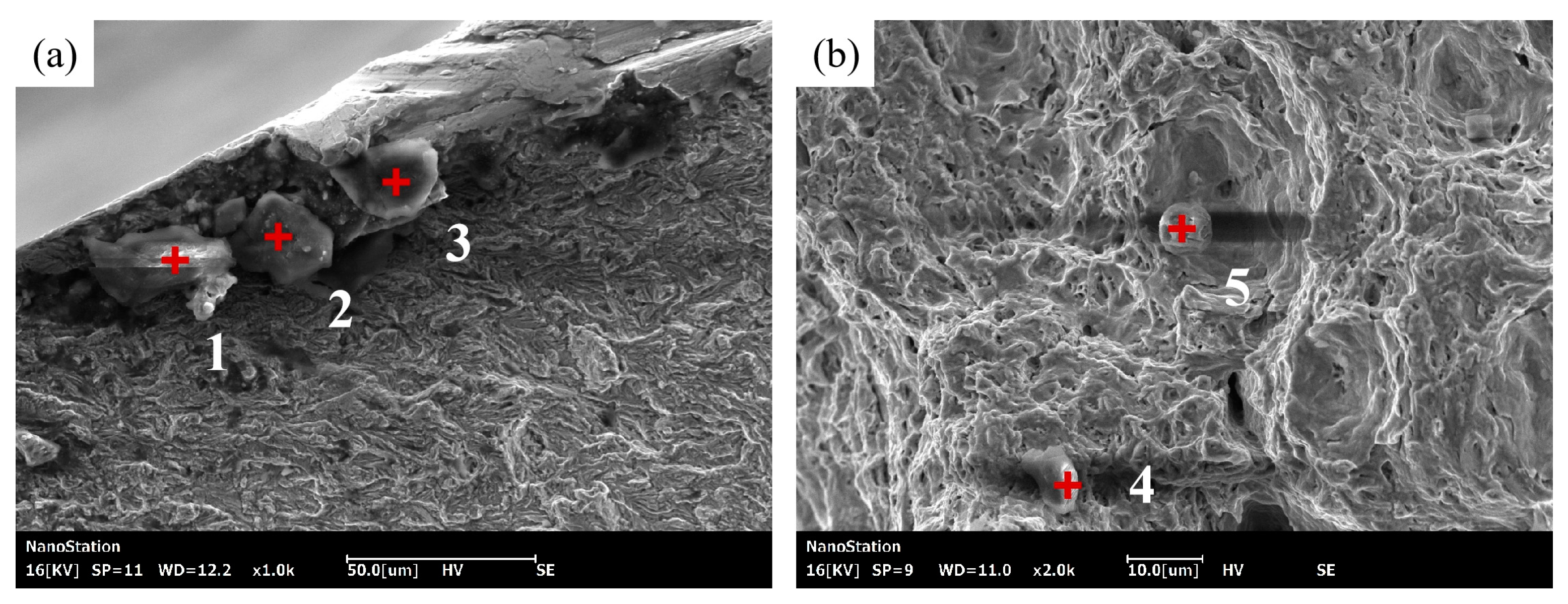
Figure 24 showed the morphology of inclusions at location 1, 2, 3, 4 and 5 in the I and II zones. From the figure, it can be seen that inclusions at location 1, 2 and 3 were irregular block-shaped with sizes between 25-40 μm, while inclusions at location 4 and 5 were ellipsoidal and spherical with diameters between 6-10 μm, with the former being much larger than the latter. Table 8 showed the energy spectrum analysis results of the inclusions at different location in Figure 24. Based on the results in the table, it was inferred that the inclusions at locations 1, 2, and 3 were composite inclusions consisting of CaO, SiO2, TiO2, and FeS [29,46]. The location and content of these inclusions were relatively close, which may be due to a large block inclusion undergoing deformation and splitting into three smaller inclusions because of stress concentration during the fatigue test, becoming the source of fatigue failure in the steel [47]. The inclusion at location 4 was speculated to be primarily composed of SiO2, Al2O3, and a small amount of TiO2. It was suggested that this inclusion was mainly formed due to secondary oxidation of silicon and the precipitation of dissolved oxygen during the steel refining process, resulting in the formation of glassy silicate inclusions rich in SiO2. The inclusion at location 5 was inferred to have a core composition of Al2O3·CaO·MgO·TiO2, with the deposition of composite inclusions such as MnS on its surface [48].

Table 8.
Energy spectrum analysis results of inclusions in Figure 24.
Table 8.
Energy spectrum analysis results of inclusions in Figure 24.
| Location | Element ( at%) | |||||||||||
|---|---|---|---|---|---|---|---|---|---|---|---|---|
| Fe | C | O | Ti | S | Ca | Si | K | Cl | Al | Mg | Mn | |
| 1 | 1.01 | 79.45 | 17.86 | 0.08 | 0.48 | 0.12 | 0.42 | 0.16 | 0.27 | 0.13 | - | - |
| 2 | 0.32 | 72.70 | 25.30 | 0.09 | 0.33 | 0.24 | 0.27 | 0.10 | 0.65 | - | - | - |
| 3 | 1.40 | 82.51 | 14.08 | 0.07 | 0.53 | 0.13 | 0.39 | 0.25 | 0.64 | - | - | - |
| 4 | 1.42 | 23.82 | 58.55 | 0.040 | - | - | 13.82 | 0.53 | - | 1.82 | - | - |
| 5 | 1.24 | 28.74 | 45.25 | 0.230 | 0.19 | 4.69 | - | - | - | 18.95 | 0.59 | 0.110 |
Figure 24.
Inclusions in different zones of fatigue fracture under the maximum stress of 590 MPa (a) I zone; (b) II zone.
Figure 24.
Inclusions in different zones of fatigue fracture under the maximum stress of 590 MPa (a) I zone; (b) II zone.
4. Conclusions
This study focused on TMCP process of FH36 ship plate steel. Through tensile tests in both RD and TD directions, fatigue tests at room temperature (20℃) and low temperature (-60℃), and analysis and comparison of the morphology, grain boundaries, and texture of the tensile and fatigue specimens, the following main conclusions were drawn:
- By adopting the process of first rolling in the RD and then rolling in the TD, the differences properties of the steel plate in the RD and TD were effectively eliminated, resulting in almost identical tensile properties in the RD and TD at a thickness of 1/4 of the steel plate. The yield and tensile strength of the steel plate were approximately 420 MPa and 506 MPa, respectively, and the elongation was approximately 25%.
- The fatigue limit of the steel plate at room temperature was 488 MPa. When the maximum stress was below 500 MPa and above 520 MPa, the specimens failed under high-cycle and low-cycle fatigue, respectively. The high cycle fatigue fracture exhibited a oblique shearing fracture, while the low cycle fatigue fracture was a cup-cone shape, and the I zone were both on the surface of the specimens. As the maximum stress increased, the area of the II zone for high-cycle fatigue decreased, while the area of the III zone increased, and the number of dimples in the III zone increased. The proportion of the LAGBs in the fracture surfaces of high and low cycle fatigue specimens had significantly increased.
- The fatigue limit of the steel plate at -60℃ reached 500 MPa, which was higher than the fatigue limit at room temperature indicating that its low temperature fatigue performance was better than that at room temperature. The specimens showed high-cycle and low-cycle fatigue failure when the maximum stress was below 560 MPa and above 590 MPa, respectively. The surface of the high-cycle fatigue fracture was flat, and the I zones were all on the surface of the specimen. As the applied maximum stress increased, the boundary between the II and III zones became less distinct, and the number of dimples in the III increased. The low-cycle fatigue fracture surface exhibited significant plastic deformation and multiple I zones.
Author Contributions
Conceptualization, Z.W., G.L., L.Y., P.Z. and J.Z.; methodology, Z.W., W.Z., B.L. and X.H.; software, W.Y.; validation, Z.W.; formal analysis, W.Y. and D.W.; investigation, D.W.; resources, Z.W.; data curation, W.Y.; writing—original draft preparation, W.Y.; writing—review and editing, D.W.; visualization, W.Y. and D.W.; supervision, Z.W.; project administration, Z.W.; funding acquisition, Z.W. and L.Y. All authors have read and agreed to the published version of the manuscript.
Funding
This study was funded by the University of Science and Technology Liaoning-State Key Laboratory of Metal Material for Marine Equipment and Application Joint Fund, grant number HGSKL-USTLN(2020)03, and by the National Natural Science Foundation of China, grant number 51204095.
Acknowledgments
The authors gratefully acknowledge University of Science and Technology Liaoning-State Key Laboratory of Metal Material for Marine Equipment and Application Joint Fund for the financial support of this work.
References
- Wang, K.; Wu, L.; Li, Y.; Qin, C. Experimental study on low temperature fatigue performance of polar icebreaking ship steel. Ocean Eng. 2020, 216, 107789. [Google Scholar] [CrossRef]
- Qin, C. Study on low temperature fatigue performance of steel used in polar icebreaker. Master's Thesis, Jiangsu University of Science and Technology, Zhenjiang, China, 2020. [Google Scholar]
- Wang, D.; Zhang, P.; Peng, X.; Yan, L.; Li, G. Comparison of microstructure and mechanical properties of high strength and toughness ship plate steel Materials, Materials 2021, 14, 5886.
- Xu, G.; Yan, R.; Yao, G.; Dong, Q. Theoretical and Experimental Study on CTOD for Notch Plate Under Low Cycle Fatigue. J. Ship Mechanics 2017, 21, 1128–1135. [Google Scholar]
- Wang, S.; Peng, X.; Zhang, P. Analysis of fatigue resistance of fh36 shipbuilding steel plate. Foundry Technol. 2022, 43, 531–536. [Google Scholar]
- Le, J.; Tu, W.; Xie, H.; Yang, K.; Tang, W. Simulation and experimental study on fatigue crack propagation of marine high-strength steel under variable amplitude loading. Proceedings of the symposium on ship structural mechanics. 2019, 18–23. [Google Scholar]
- Jiang, F.; Liu, R. Low cycle fatigue behavior of marine steel 945. Appl. Sci. & Technol. 1995, 1-5. 1995.
- Li, Z.; Sun, J.; Hu, X.; Zheng, F.; Zhang, H. Gigacycle fatigue of high strength steel 65Mn. Appl. Sci. & Technol. 2007, 54-56.
- Wang, Y.; Feng, G.; Ren, H. Experiment of influence of specimen thickness on fatigue crack propagation rate of ship hull steel. Ship Engineering 2019, 41, 98–104. [Google Scholar]
- GB/T 228.1-2010 Metallic materials-tensile testing-Part 1: Method of test at room temperature; China Standard Press: Beijing, China, 2011.
- GB/T 3075-2008 Metallic materials: fatigue testing:axial-force-controlled method; China Standard Press: Beijing, China, 2008.
- Gao, Z.; Xiong, J. Fatigue reliability; Beihang University Press: Beijing, China, 2013; pp. 138–139. [Google Scholar]
- Yao W.Fatigue life prediction of structures; National Defense Industry Press: Beijing, China, 2003; pp. 50–54.
- Zhang, J. Effects of aging process on microstructure and fatigue properties of 7N01 aluminum alloy. Master's Thesis, . Harbin Institute of Technology, Harbin, China, 2020. [Google Scholar]
- Li W, Lu L. Research on Ultra-Long Life Duplex S-N Curve Model. China Railway Science 2008, 101-105.
- Little R E, Jebe E H. Statistical design of fatigue experiments; Applied Science Publishers LTD: London, England, 1975; pp. 61–80.
- Ling, J.; Gao, Z. Maximum Likelihood Method for Measuring P-S-M curve. Acta Aeronaut. Astronaut. Sin. 1992, 247–252. [Google Scholar]
- Zheng, R.; Qin, Z. Grey Method for Fitting S-N Curve. J. National Univ. Defense Technol. 1989, 84–88. [Google Scholar]
- Xie, J.; Yao, W. Double Weighted Least Square Method for Fatigue S-N Curve Fitting. Journal of Astronautics 2010, 31, 1661–1665. [Google Scholar]
- Gao, Z.; Fu, H.; Liang, M. A Method For Fitting S-N Curve. J B Univ Aeronaut Astronaut. 1987, 115–119. [Google Scholar]
- GB/T 712-2011 Ship and ocean engineering structural steel; China Standard Press: Beijing, China, 2011.
- Xu, B. Surface engineering and maintenance; China Machine Press: Beijing, China, 1996; p. 148. [Google Scholar]
- Wang, J. Principles and experiments of mechanical properties of materials; Tianjin University Press: Tianjin, China, 2018; p. 49. [Google Scholar]
- Cui, Y.; Wang, C. Metal fracture analysis; Harbin Institute of Technology Press: Harbin, China, 1998; p. 28. [Google Scholar]
- Li, J.; Wei, C.; Zhang, W.; Li, P. Analysis of inclusions in steel and properties and fracture of steel; Metallurgical Industry Press: Beijing, China, 2012; p. 64. [Google Scholar]
- Luo D. Study on Mechanism of Yttrium-based Rare Earth on Inclusions Behavior and Microstructure and Properties of EH36 Shipbuilding Steel. Doctor's Thesis. Jiangxi University of Science and Technology, Ganzhou, China, 2022.
- Technical Training and Qualification Assessment Committee for Mechanical Industry Physical and Chemical Testing Personnel, Physical and Chemical Testing Branch of the Chinese Mechanical Engineering Society. Chemical Analysis of Metallic Materials; Popular Science Press: Beijing, China, 2015; pp. 244.
- Wang, D.; Li, G.; Yin, W.; Yan, L.; Wang, Z.; Zhang, P.; Hu, X.; Li, B.; Zhang, W. Studying on Alloying Elements, Phases, Microstructure and Texture in FH36 Ship Plate Steel. Materials 2023, 16, 4762. [Google Scholar] [CrossRef] [PubMed]
- Wu, R.; Wu, Z. Steel quality and failure analysis of its components; Beihang University Press: Beijing, China, 2018; pp. 143 and 160.
- Wang, D. The Analysis of Breakage on 851 Blade of 300MW Steam Turbine. Shandong Electric Power 1996, 68–70. [Google Scholar]
- Bai, R.; Cai, G.; Zhang, X.; Chen, W.; Jiang, Y. Numerical simulation analysis of asymmetric fatigue failure for iced electric power transmission line. Chin. J Mater. Study 2016, 30, 149–155. [Google Scholar]
- Liu, X.; Zhang, Z.; Tao, C. Fatigue fracture quantitative analysis; National Defense Industry Press: Beijing, China, 2010; p. 26. [Google Scholar]
- Encyclopedia of China Publishing House Editorial Office. Encyclopedia of China concise edition; Encyclopedia of China Publishing House: Beijing, China, 1998; pp. 3729.
- Yang, R.; Yang, F. Failure analysis and material selection; Shanghai Jiaotong University Press: Shanghai, China, 2014; p. 46. [Google Scholar]
- Xu, P. Design principles and applications of removable partial dentures and complete dentures; Peking University Health Science Center and Peking Union Medical College Associated Press: Beijing, China, 2000; p. 150. [Google Scholar]
- Xia, H. Automobile mechanical maintenance skills training course; National Defense Industry Press: Beijing, China, 2006; p. 132. [Google Scholar]
- Sha, G. Mechanical properties of materials; Beijing Institute of Technology Press: Beijing, China, 2015; p. 103. [Google Scholar]
- Wu, Y. Fracture and fatigue; China University of Geosciences Press: Wuhan, China, 2008; p. 120. [Google Scholar]
- Chen, L. Very high cycle fatigue and fracture; National Defense Industry Press: Beijing, China, 2017; p. 79. [Google Scholar]
- Nishijima, S.; Kanazawa, K. Stepwise S-N curve and fish -eye failure in gigacycle fatigue. Fatigue Fract. Eng. M. 1999, 22, 601–607. [Google Scholar] [CrossRef]
- Sun, J.; Wang, S.; Liu, P.; Wang, J.; Xiao, C.; Sun, Z.; Yu, Z. Investigation of Fatigue S-N Curves On 400 MPa Fine-Grained high Strength Rebar. Industrial Construction 2014, 44, 951–953. [Google Scholar]
- Yin, H.; Wu, Y.; Zhang, G.; Li, X.; Zhang, P.; Zhang, H.; Li, W. Effect of low temperature on fatigue properties of EA4T axle steel. China railway science 2021, 42, 123–129. [Google Scholar]
- Zhao, S.; Wang, Z. Fatigue design; China Machine Press: Beijing, China, 1992; p. 189. [Google Scholar]
- Zhang, D.; Zhong, P. Practical Analysis of mechanical failure; National Defense Industry Press: Beijing, China, 1997; p. 143. [Google Scholar]
- Wang, S.; Han, J.; Zeng, W.; Zhang, X.; Zhao, J.; Dai, G. Effect of low temperature on mechanical properties of ER8 steel for wheel rim. Chin. J Mater. Study 2018, 32, 401–408. [Google Scholar]
- Fu C.; Dong W.; Wu J.; Zhu L. Inspection Defect Analysis of Class B Ship Plate produced in TISC. Tianjin Metallurgy 2019, 37-40+90.
- Liu, X. Study on precipitation behavior of MnS inclusions in steel. Master's Thesis, Northeastern University: Shenyang, China, 2012; p. 7. [Google Scholar]
- Zhang, L. Non-Metallic Inclusions in Steel Industrial Practice; Metallurgical Industry Press: Beijing, China, 2019; p. 154. [Google Scholar]
Figure 1.
Tensile specimen location and size.
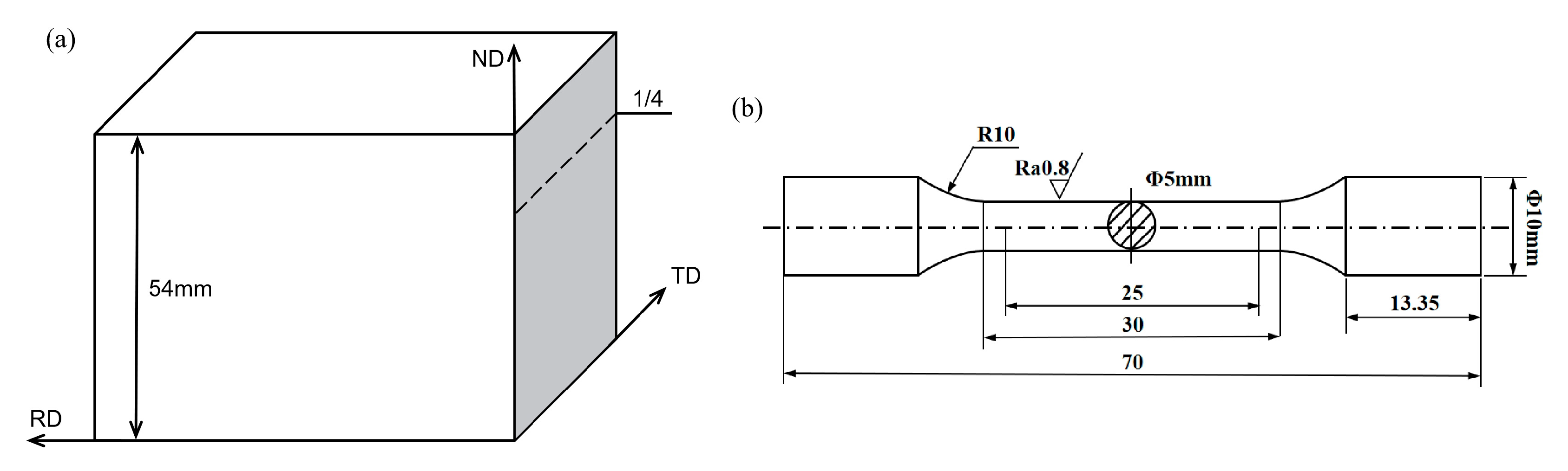
Figure 2.
Size of the fatigue specimen.
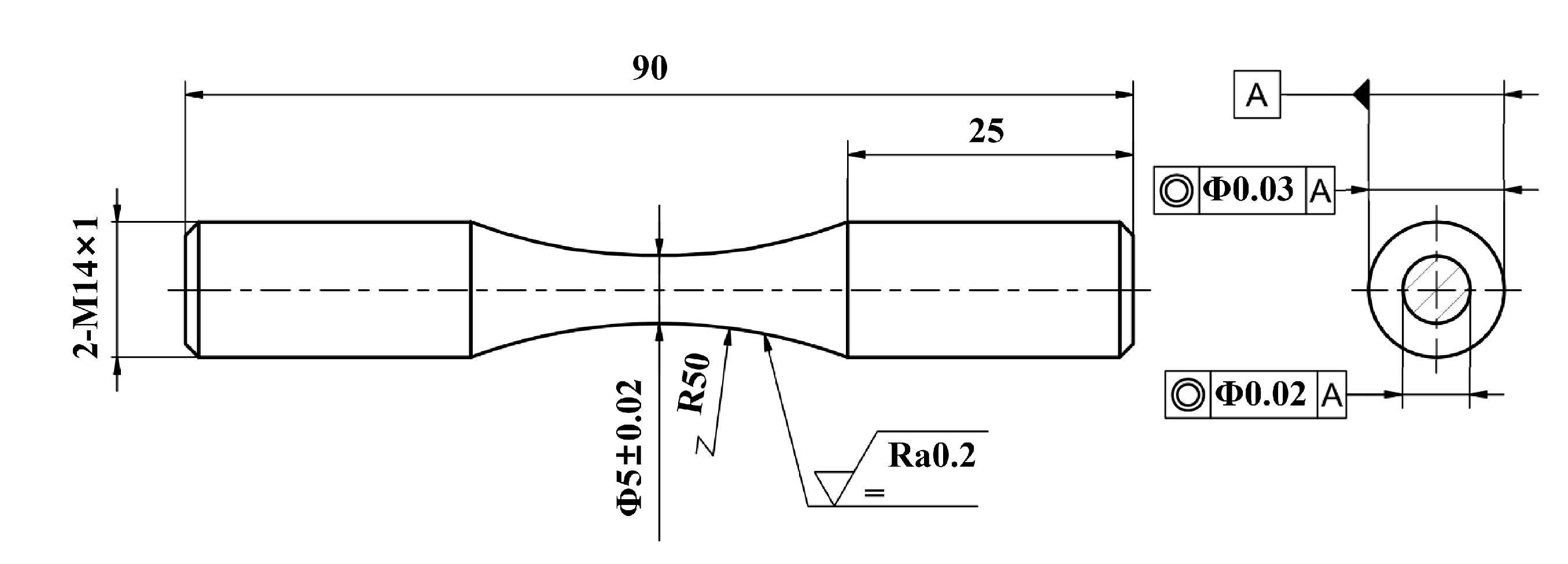
Figure 3.
Tensile stress-strain curves of the steel plate (a) RD; (b) TD.
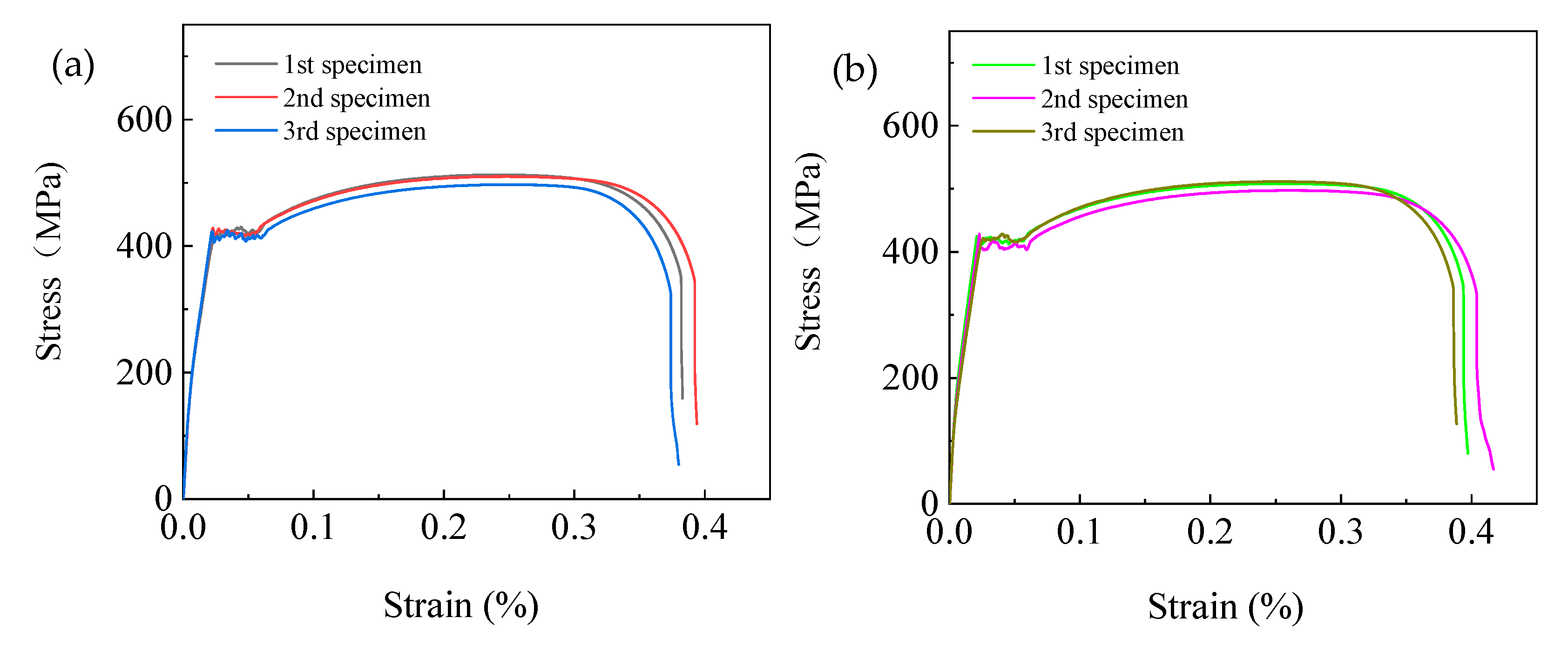
Figure 4.
Tensile test results of steel plate.
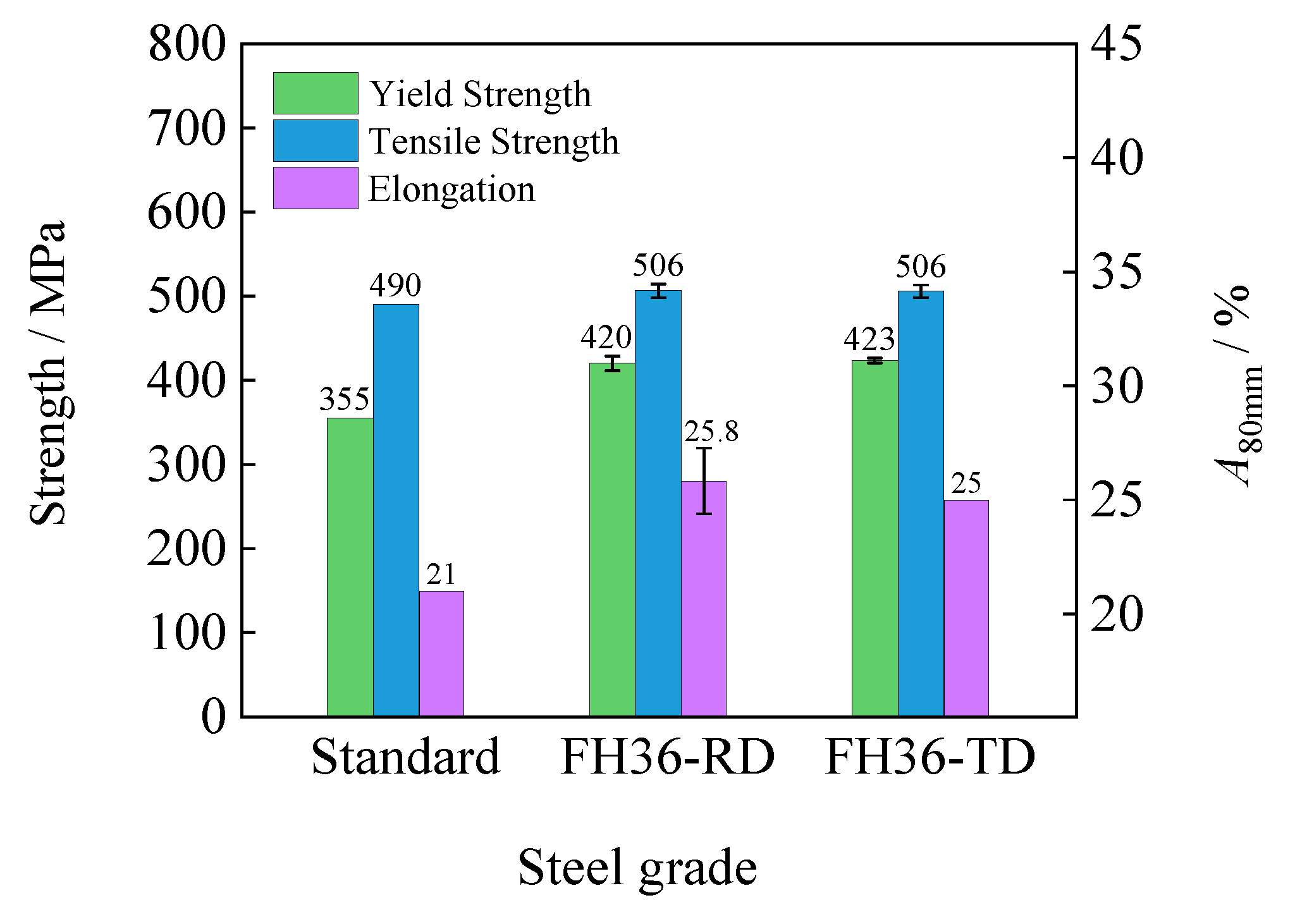
Figure 5.
Tensile fracture morphology (a,b,c) RD; (d,e,f) TD.
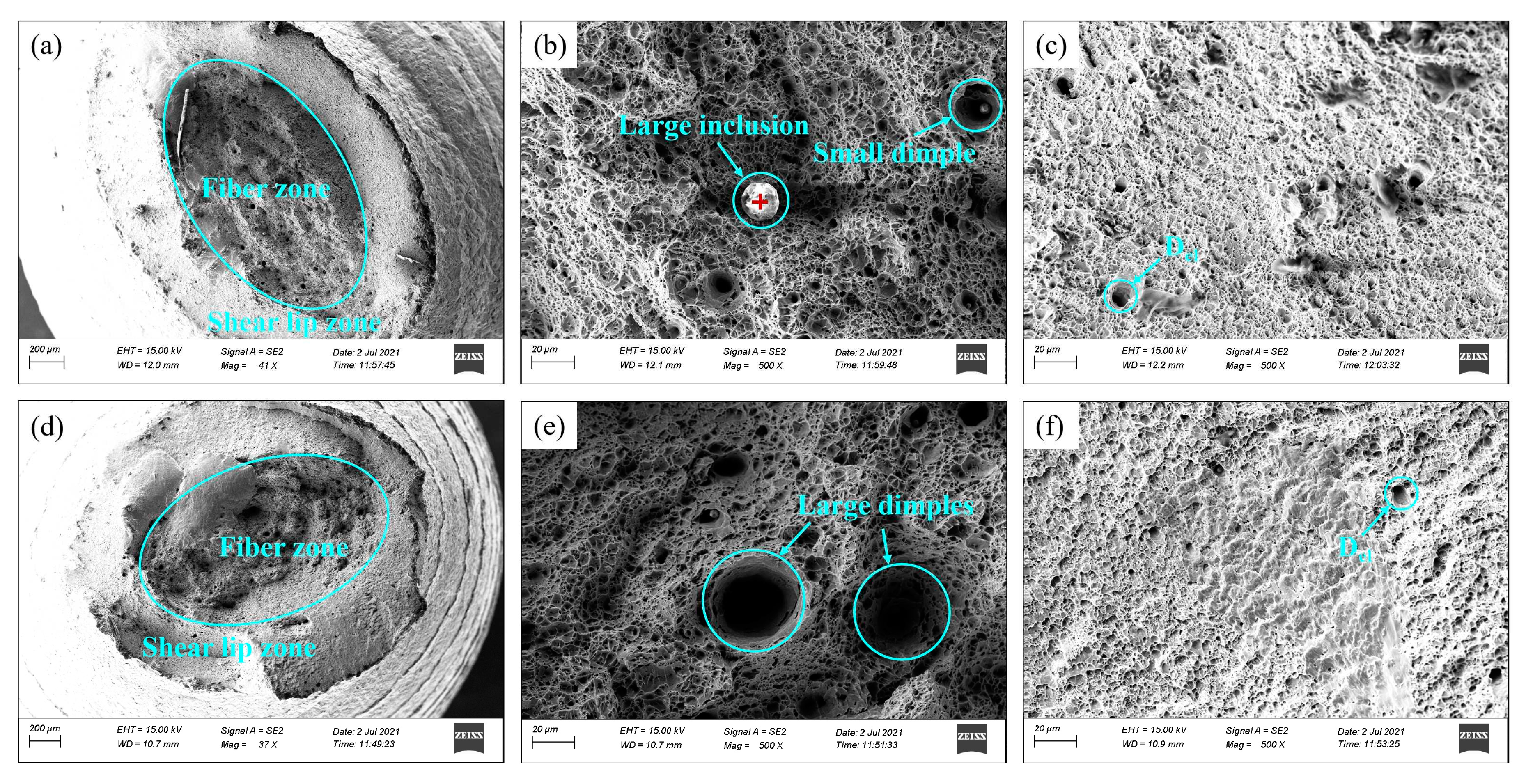
Figure 6.
Fatigue test up-and-down diagram.
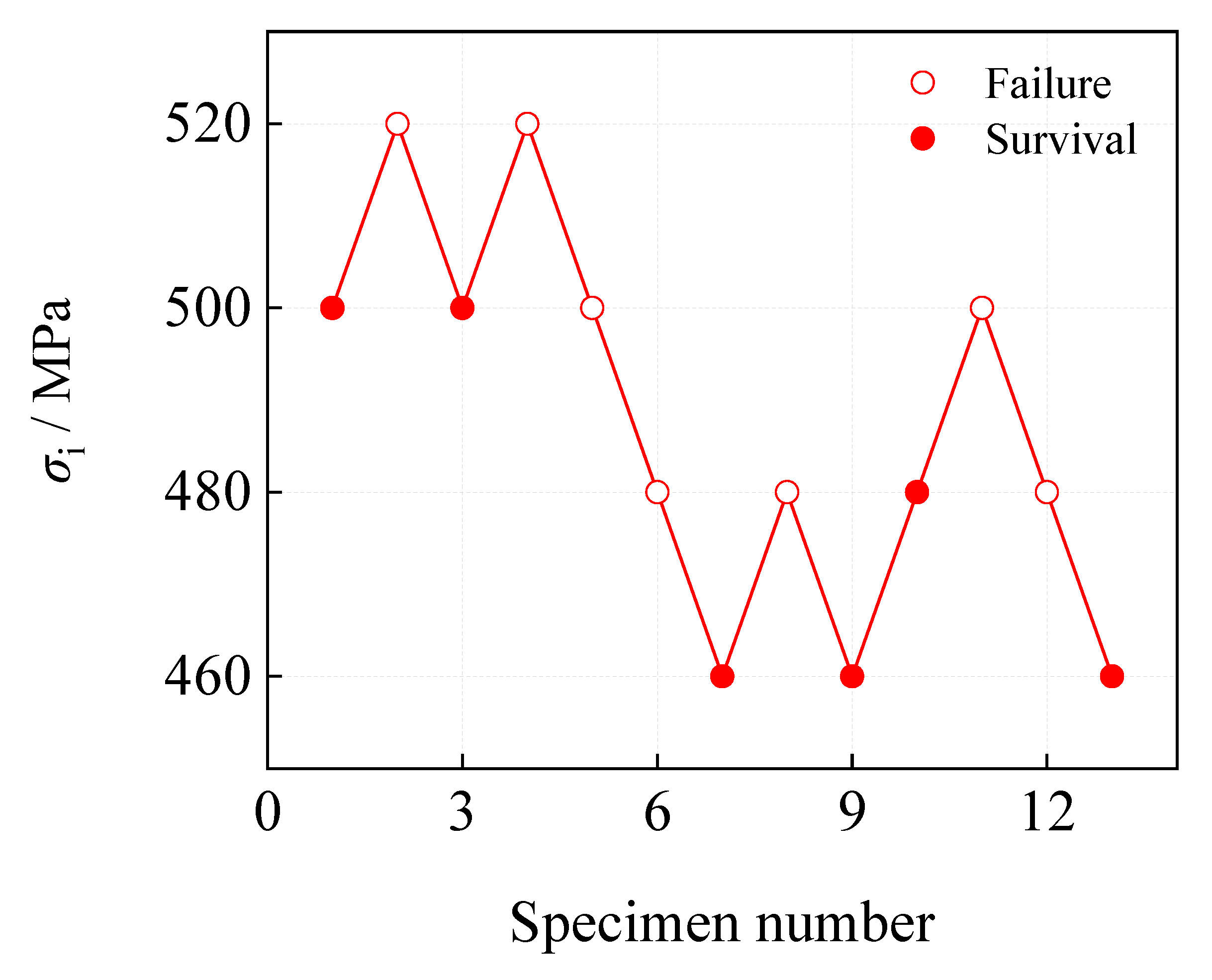
Figure 7.
Fatigue specimens at room temperature under different maximum stress: (a) 480 MPa; (b) 500 MPa; (c) 520 MPa.
Figure 7.
Fatigue specimens at room temperature under different maximum stress: (a) 480 MPa; (b) 500 MPa; (c) 520 MPa.
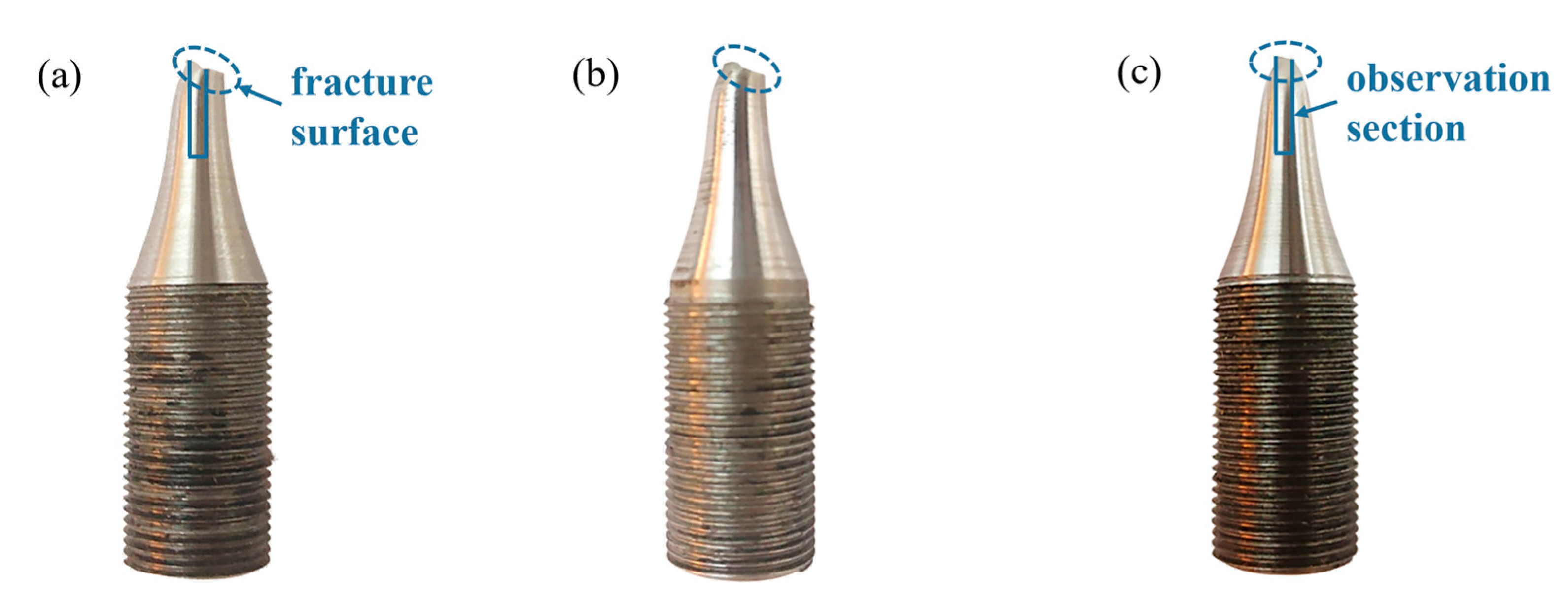
Figure 8.
Illustration of the division of fatigue fracture zones and critical crack length ac.
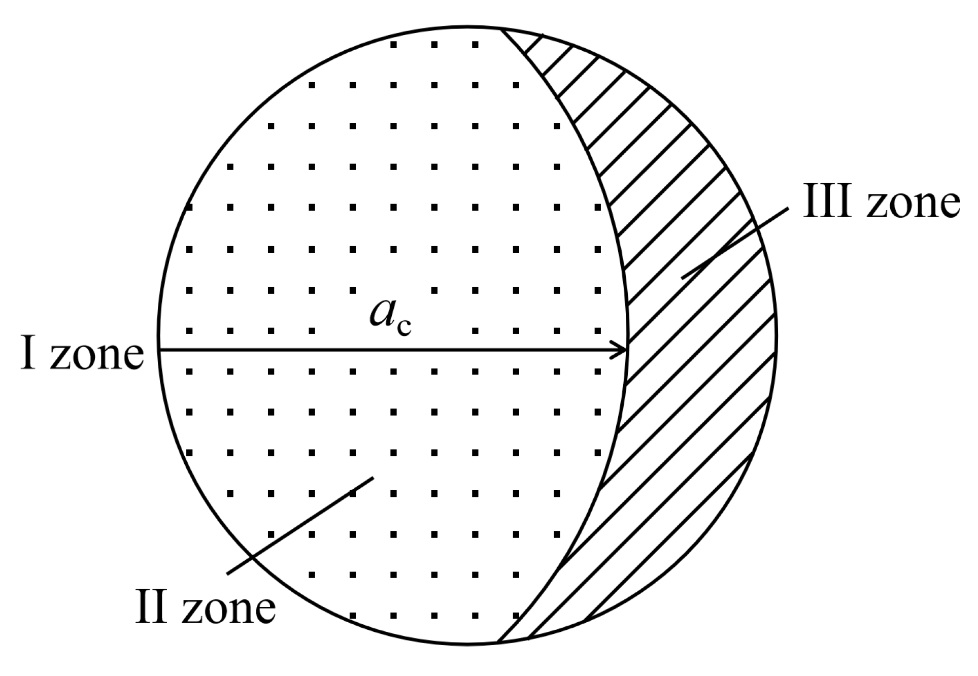
Figure 9.
Fatigue fracture morphology of the specimens under the maximum stress of 480 MPa (a,d,g) macroscopic morphology; (b,e,h) II zone; (c,f,i) III zone.
Figure 9.
Fatigue fracture morphology of the specimens under the maximum stress of 480 MPa (a,d,g) macroscopic morphology; (b,e,h) II zone; (c,f,i) III zone.
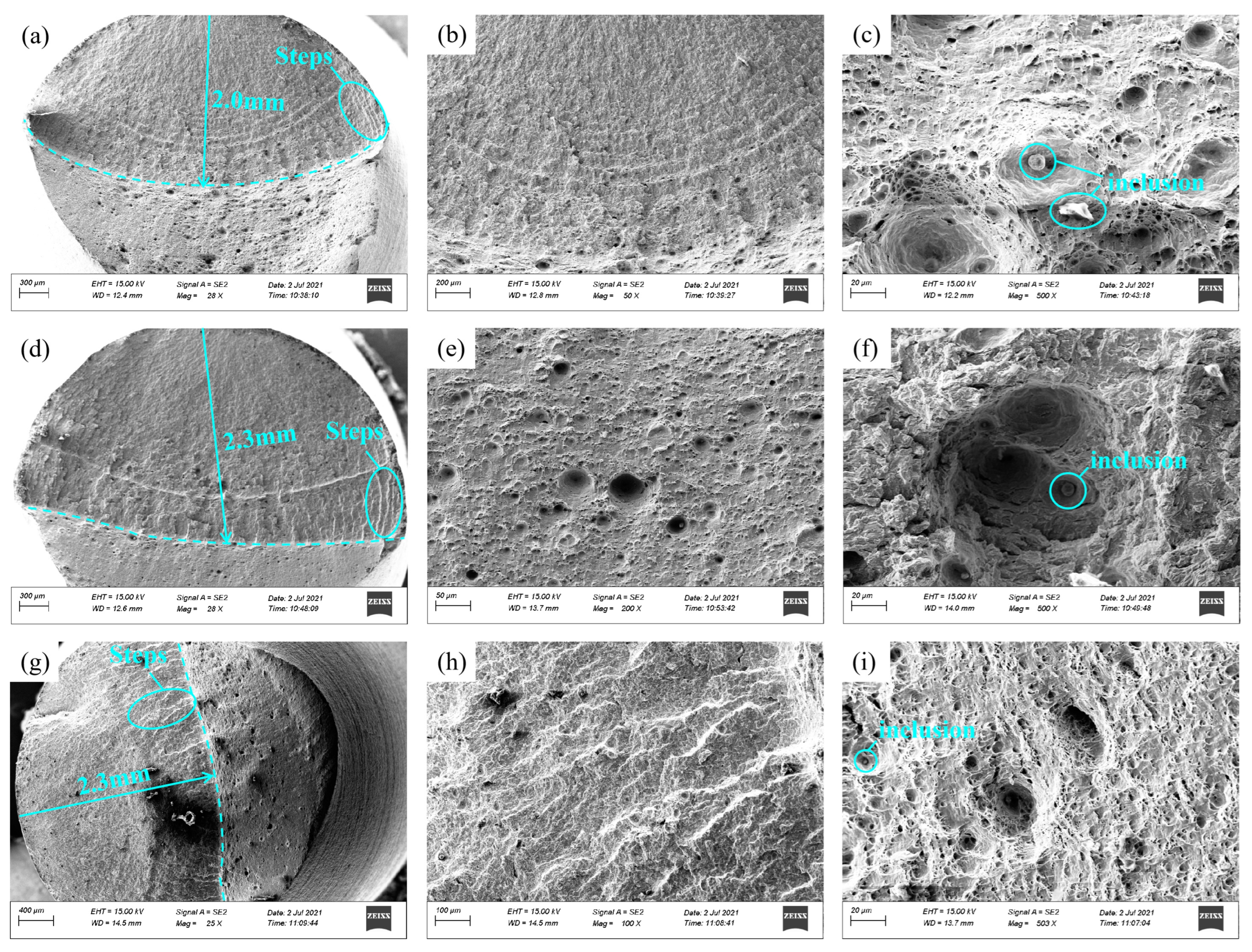
Figure 10.
Fatigue fracture morphology of specimen under the maximum stress of 500 MPa (a) macroscopic morphology; (b) II zone; (c) III zone.
Figure 10.
Fatigue fracture morphology of specimen under the maximum stress of 500 MPa (a) macroscopic morphology; (b) II zone; (c) III zone.
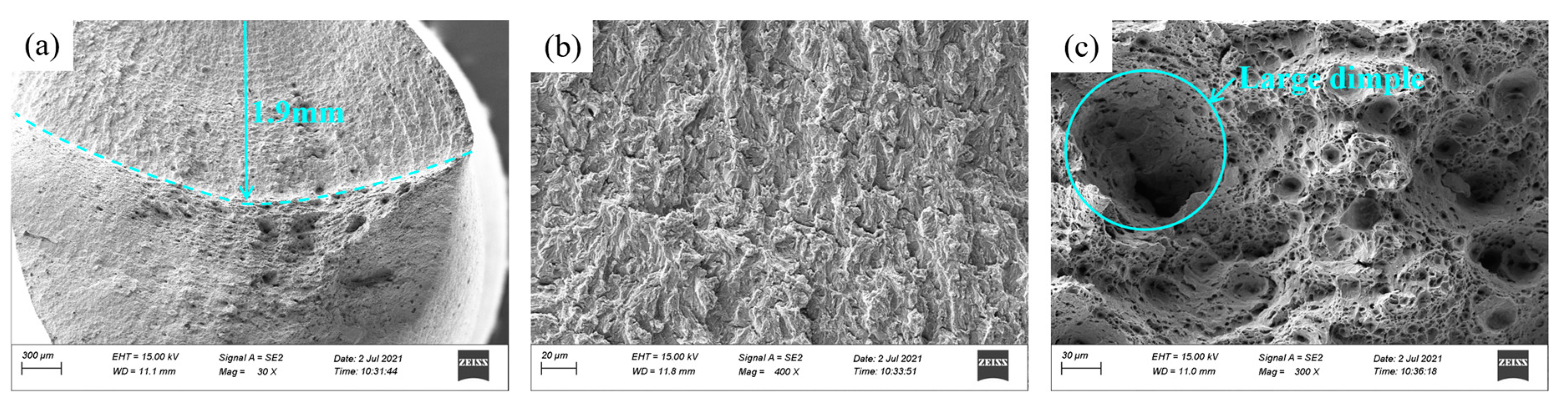
Figure 11.
Fatigue fracture morphology of the specimen under the maximum stress of 520 MPa (a, d) Macroscopic morphology; (b, e) Shear lip zone; (c, f) Fiber zone.
Figure 11.
Fatigue fracture morphology of the specimen under the maximum stress of 520 MPa (a, d) Macroscopic morphology; (b, e) Shear lip zone; (c, f) Fiber zone.
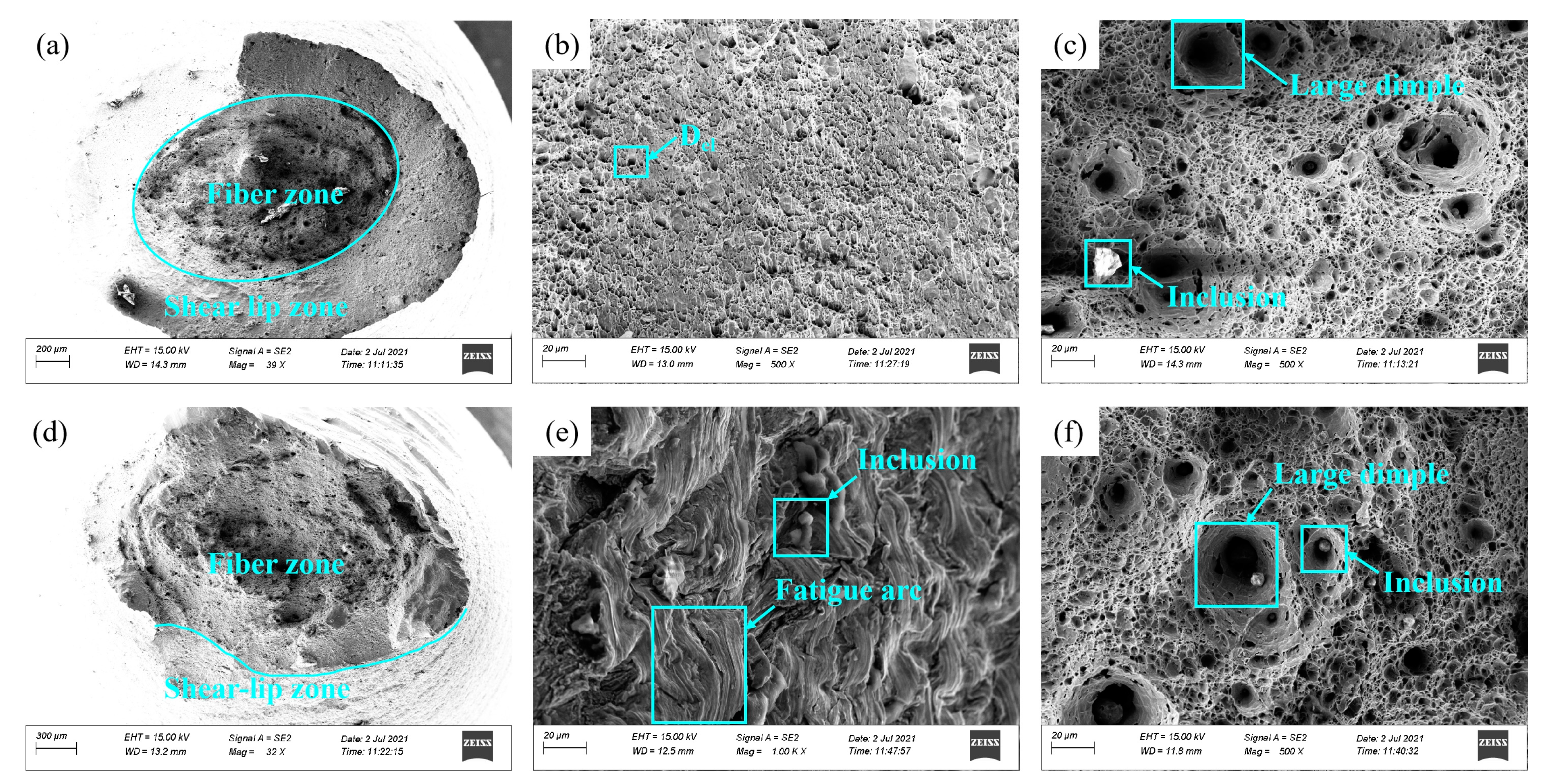
Figure 12.
Microstructure of fatigue specimens under different maximum stress (a) 480 MPa; (b) 500 MPa; (c) 520 MPa.
Figure 12.
Microstructure of fatigue specimens under different maximum stress (a) 480 MPa; (b) 500 MPa; (c) 520 MPa.
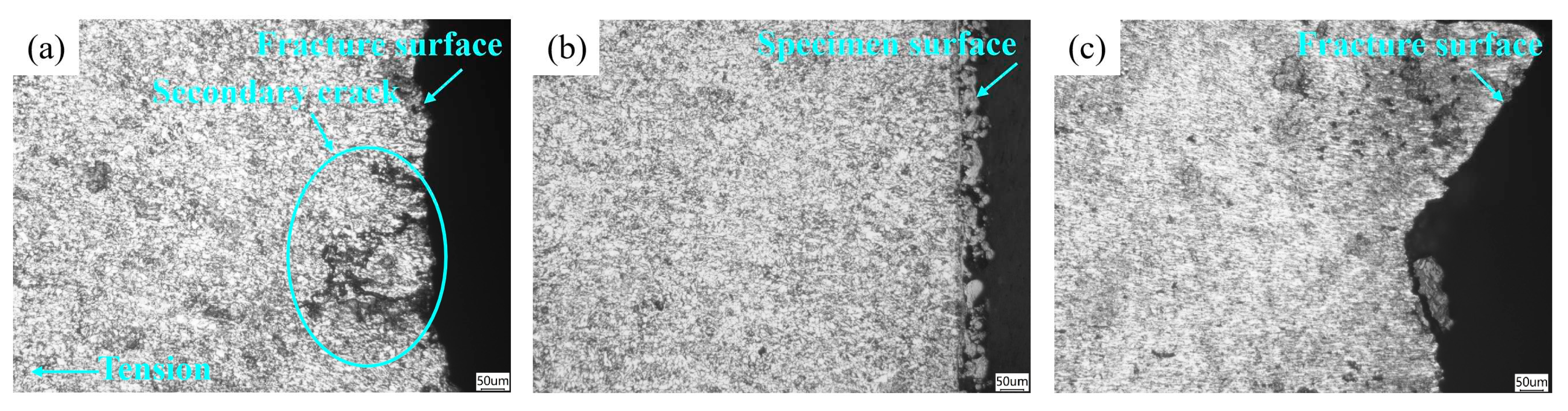
Figure 13.
Fatigue fracture cross-sectional microstructure of the specimen under the maximum stress of 520 MPa.
Figure 13.
Fatigue fracture cross-sectional microstructure of the specimen under the maximum stress of 520 MPa.
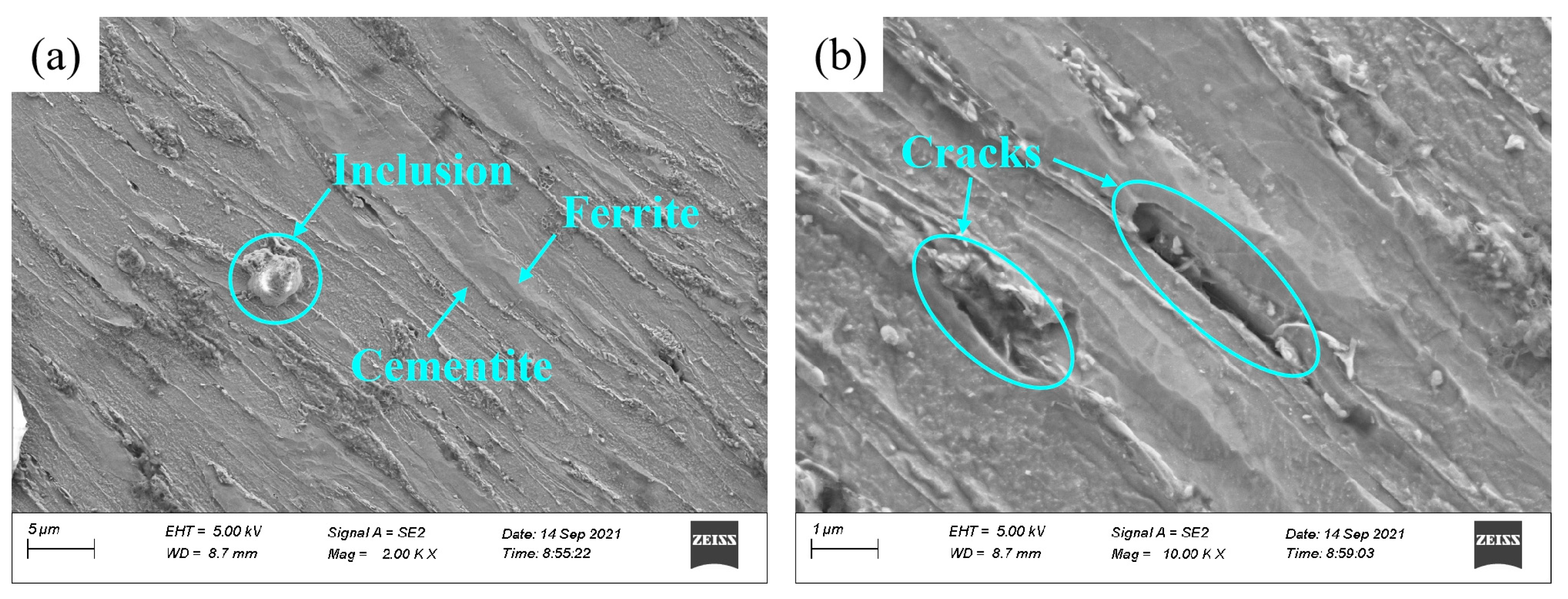
Figure 14.
IPF maps of (a) the original, (b) and (c) fatigue fracture cross-sectional specimens under the maximum stress of 480 MPa and 520 MPa.
Figure 14.
IPF maps of (a) the original, (b) and (c) fatigue fracture cross-sectional specimens under the maximum stress of 480 MPa and 520 MPa.
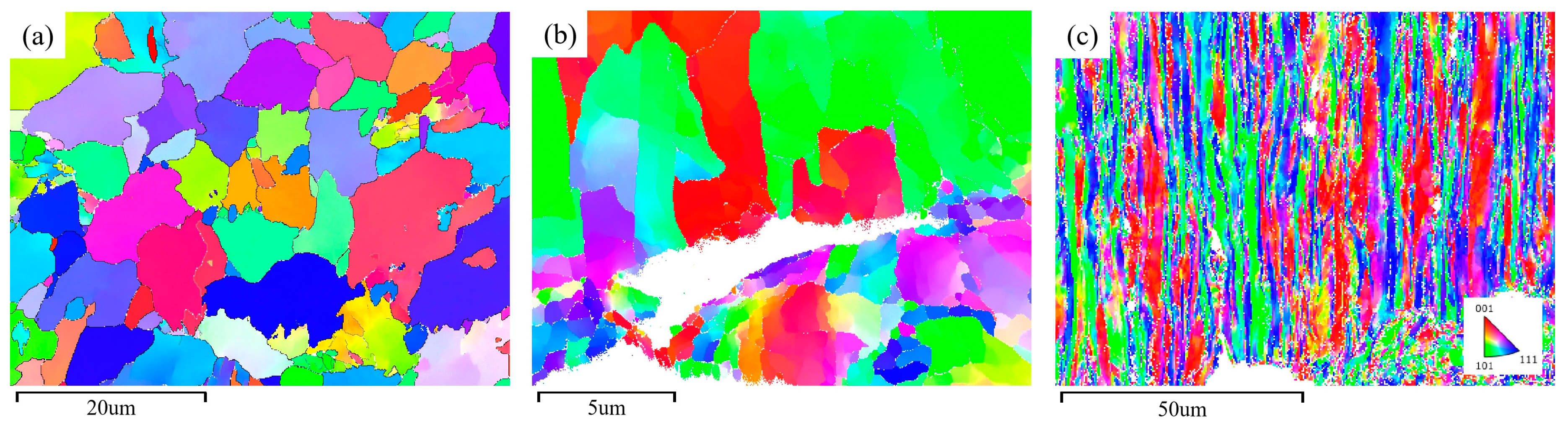
Figure 15.
Texture components and KAM maps of fatigue fracture cross-sections under different maximum stress (a)(c) 480 MPa; (b)(d) 520 MPa.
Figure 15.
Texture components and KAM maps of fatigue fracture cross-sections under different maximum stress (a)(c) 480 MPa; (b)(d) 520 MPa.
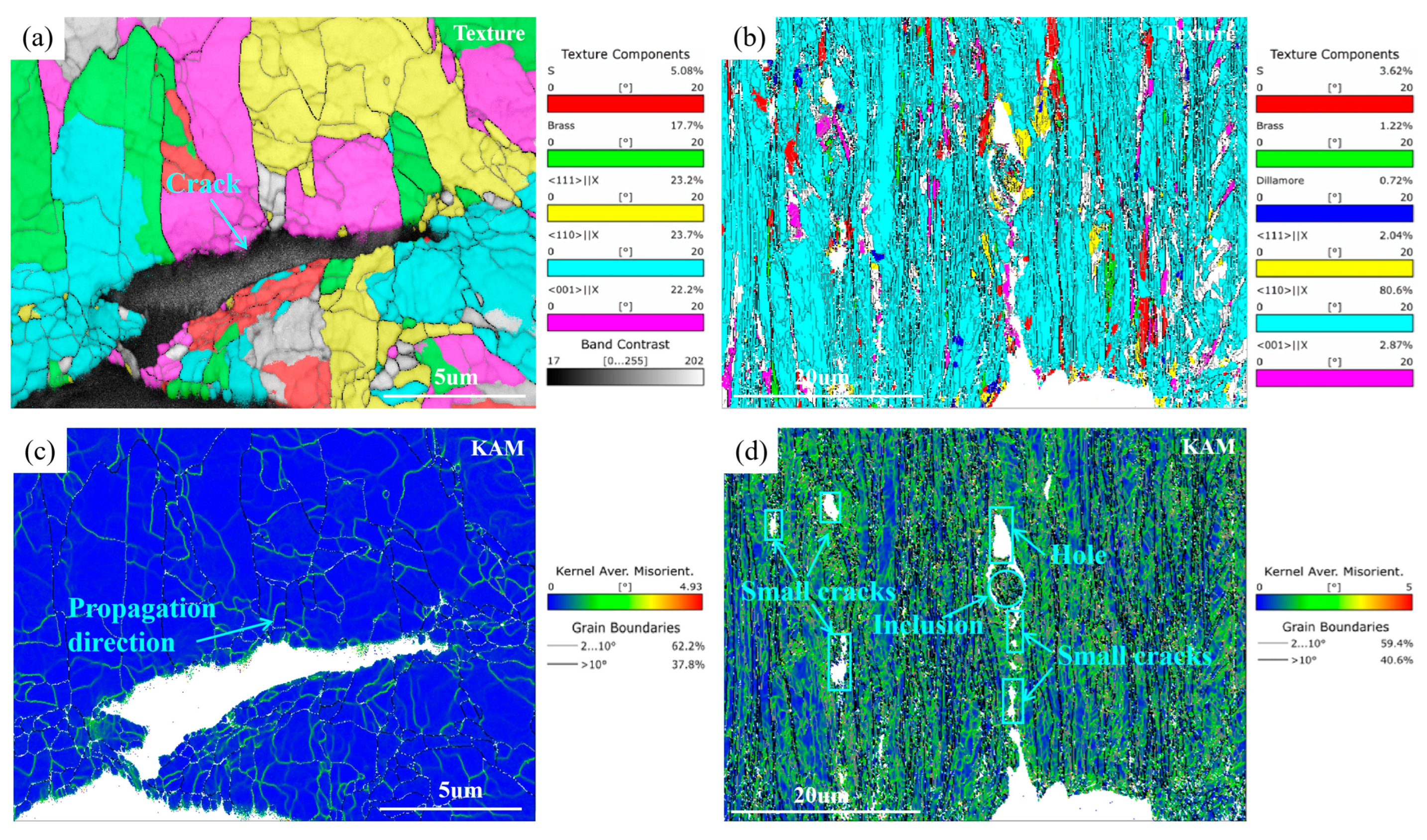
Figure 16.
Common orientation map for the cubic crystal system with the φ2 angle of 45°.
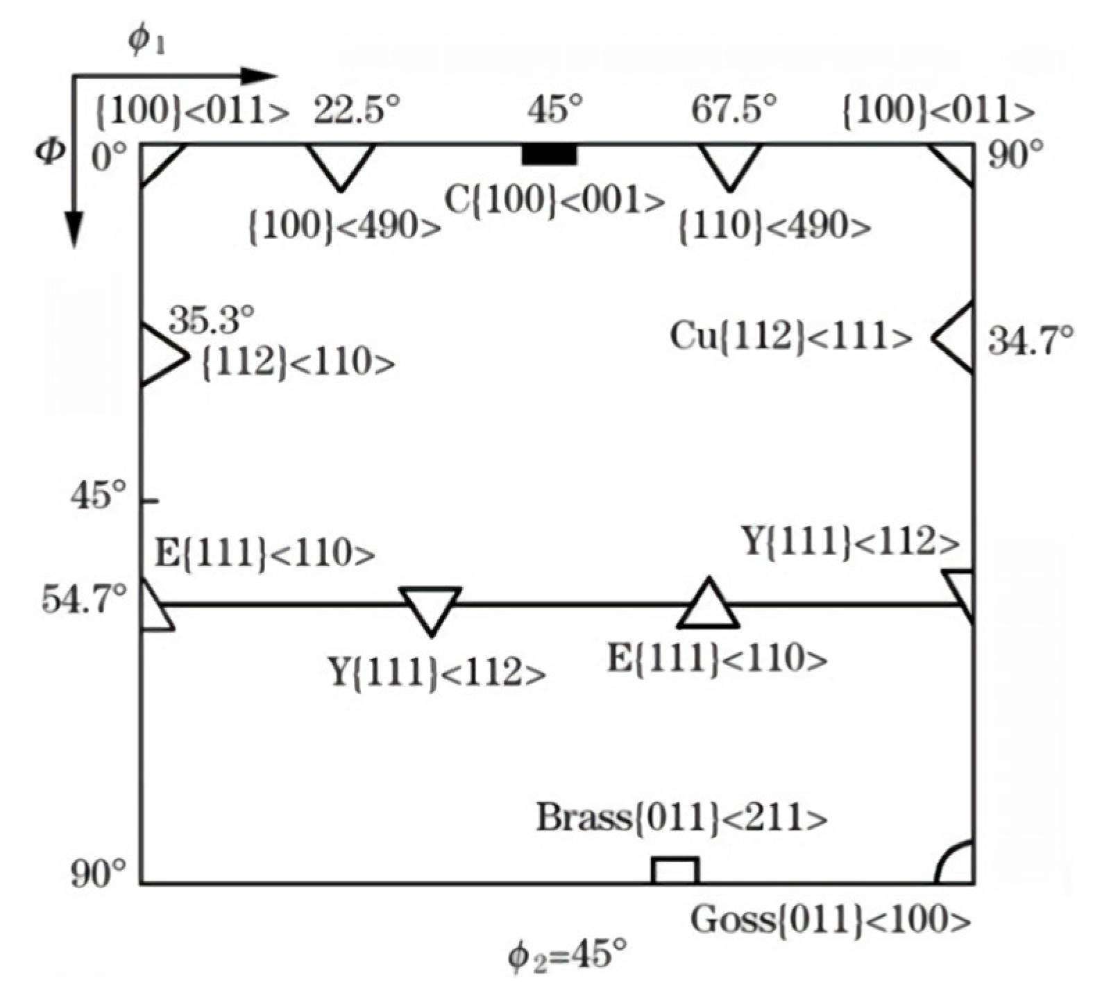
Figure 17.
ODF figures of fatigue fracture cross-sections under different maximum stress (a) 480 MPa; (b) 520 MPa.
Figure 17.
ODF figures of fatigue fracture cross-sections under different maximum stress (a) 480 MPa; (b) 520 MPa.
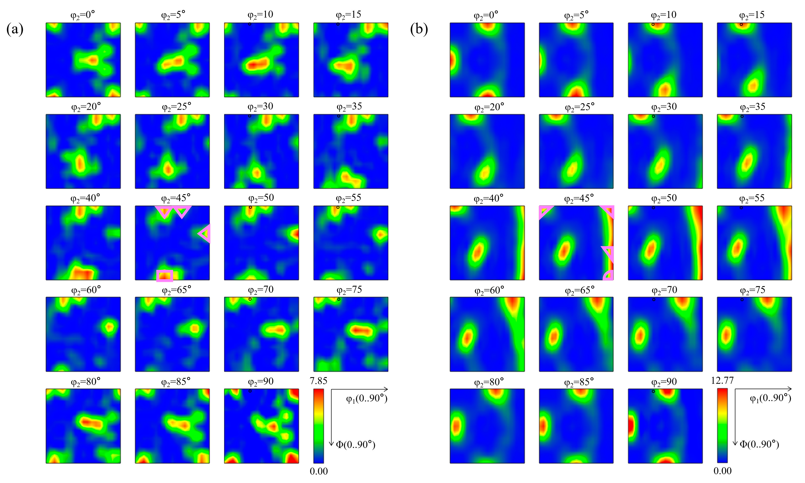
Figure 18.
Polar figures of low-cycle fatigue fracture cross-section (a) (001); (b) (110); (c) (111).
Figure 18.
Polar figures of low-cycle fatigue fracture cross-section (a) (001); (b) (110); (c) (111).
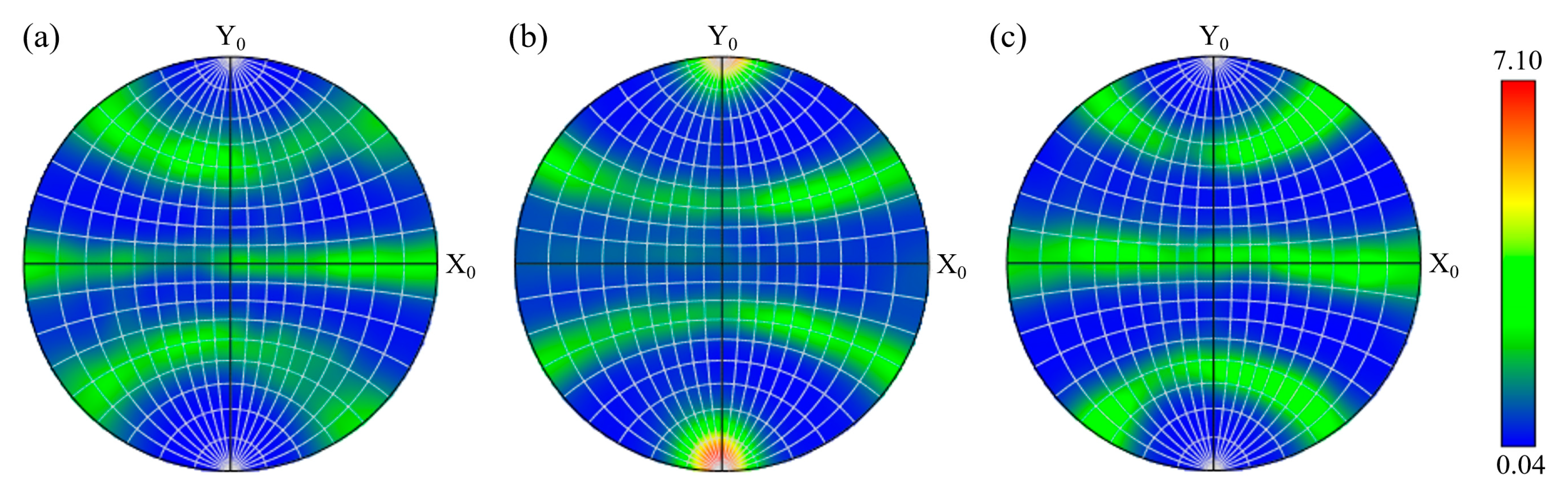
Figure 19.
S-N curve of the three-parameter model.
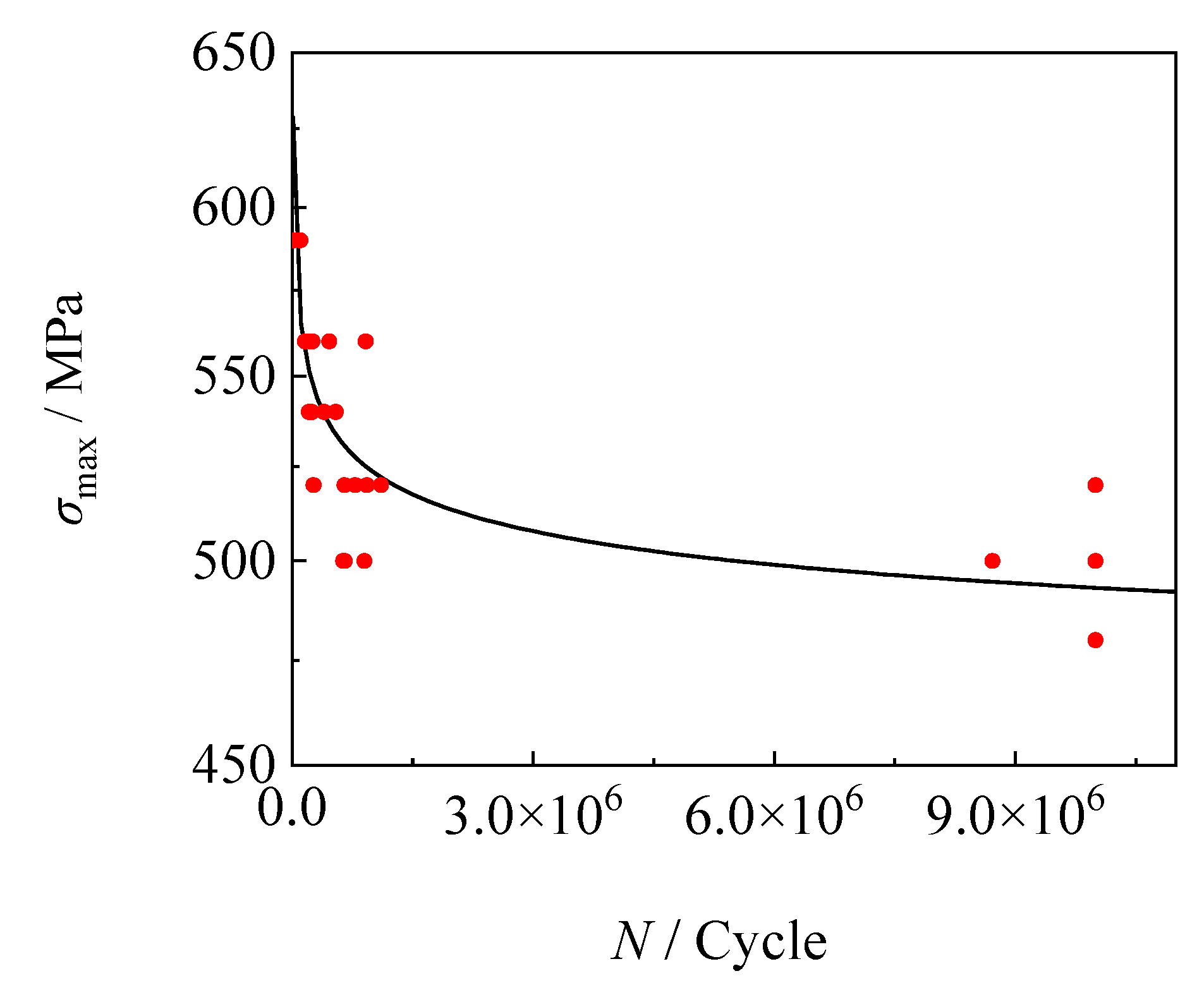
Figure 20.
Low-temperature fatigue fractured specimen under different maximum stress (a) 500 MPa; (b) 520 MPa; (c) 540 MPa; (d) 560 MPa; (e)590 MPa.
Figure 20.
Low-temperature fatigue fractured specimen under different maximum stress (a) 500 MPa; (b) 520 MPa; (c) 540 MPa; (d) 560 MPa; (e)590 MPa.
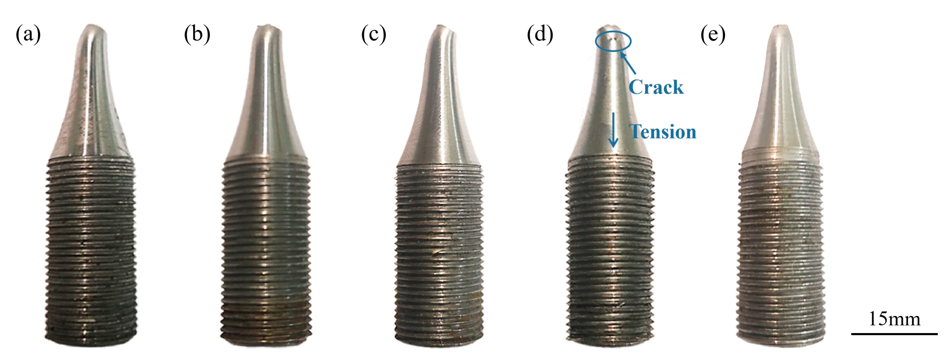
Figure 21.
(a) Side crack and (b) magnified view of the local area of the fatigue specimen.
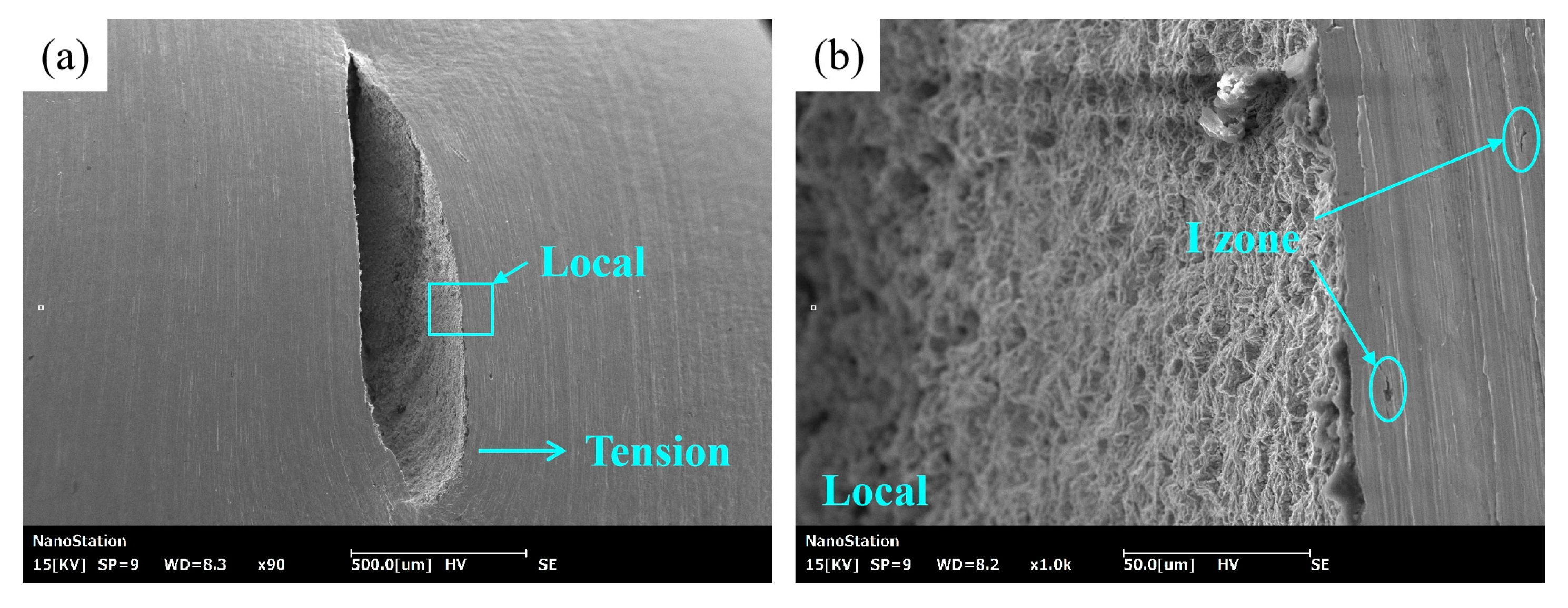
Figure 22.
High-cycle fatigue fracture morphology under different maximum stress: (a), (b), (c) 500 MPa; (d), (e), (f) 520 MPa; (g), (h), (i) 540 MPa; (j), (k), (l) 560 MPa.
Figure 22.
High-cycle fatigue fracture morphology under different maximum stress: (a), (b), (c) 500 MPa; (d), (e), (f) 520 MPa; (g), (h), (i) 540 MPa; (j), (k), (l) 560 MPa.
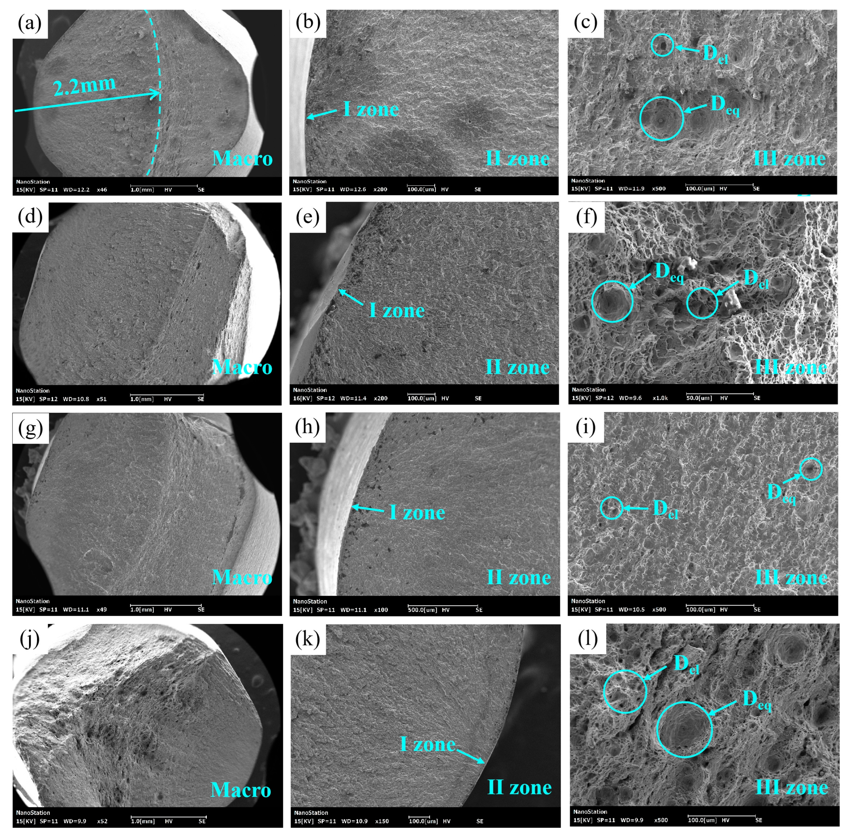
Figure 23.
Fatigue fracture morphology of the specimen under 590 MPa maximum stress: (a) Macroscopic morphology; (b) I and II zones; (c) III zone.
Figure 23.
Fatigue fracture morphology of the specimen under 590 MPa maximum stress: (a) Macroscopic morphology; (b) I and II zones; (c) III zone.
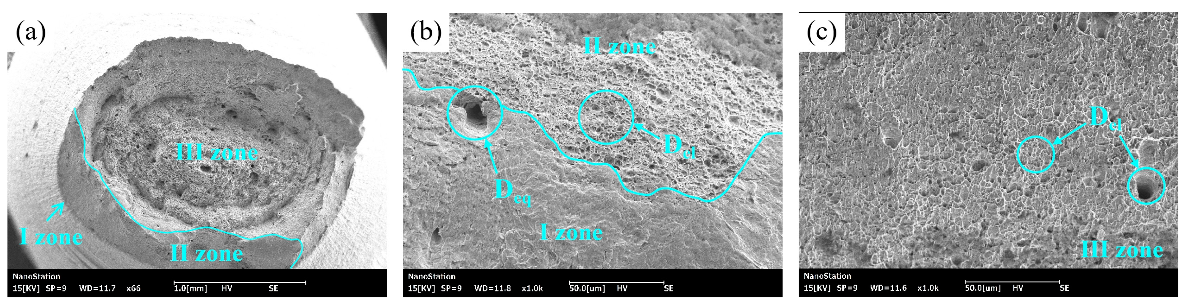
Table 1.
Chemical composition of FH36 steel plate (%).
| Chemical composition | ||||||||||||
|---|---|---|---|---|---|---|---|---|---|---|---|---|
| C | Si | Mn | S | P | Nb | V | Ti | Als | Cu | Cr | Ni | Fe |
| 0.08 | 0.17 | 1.42 | 0.002 | 0.012 | 0.03 | 0.040 | 0.013 | 0.030 | 0.10 | 0.16 | 0.35 | Bal. |
Table 2.
TMCP parameters of FH36 steel plate (℃).
| First-stage rolling temperature | Second-stage rolling temperature | Final rolling temperature | Water inlet temperature | Self-tempering temperature |
|---|---|---|---|---|
| 1050 | 830 | 790 | 760 | 500 |
Table 3.
Composition of the large inclusion in Figure 5(b).
Table 3.
Composition of the large inclusion in Figure 5(b).
| Element | C | O | Al | Si | S | Ca | Ti | Mn | Fe | Nb | Ni | Cu |
|---|---|---|---|---|---|---|---|---|---|---|---|---|
| at% | 10.91 | 43.78 | 21.1 | 0.73 | 1.85 | 13.42 | 1.01 | 0.15 | 6.87 | 0.12 | 0.01 | 0.01 |
Table 4.
Fatigue test results at room temperature.
| Specimen No. | Maximum Stress /MPa | Cycles /N | Results |
|---|---|---|---|
| RT1 | 500 | 10000000 | Pass |
| RT2 | 520 | 23695 | Failure |
| RT3 | 500 | 10000000 | Pass |
| RT4 | 520 | 23659 | Failure |
| RT5 | 500 | 292586 | Failure |
| RT6 | 480 | 4787073 | Failure |
| RT7 | 460 | 10000000 | Pass |
| RT8 | 480 | 3388534 | Failure |
| RT9 | 460 | 10000000 | Pass |
| RT10 | 480 | 10000000 | Pass |
| RT11 | 500 | 167802 | Failure |
| RT12 | 480 | 537316 | Failure |
| RT13 | 460 | 10000000 | Pass |
Table 5.
Fatigue failure types under different maximum stress at room temperature.
| Temperature | Maximum Stress / MPa | |||
|---|---|---|---|---|
| 460 | 480 | 500 | 520 | |
| 20℃ | High -cycle fatigue | High -cycle fatigue | High -cycle fatigue | Low -cycle fatigue |
Table 6.
Low-temperature fatigue test results.
| Specimen No. | Maximum Stress / MPa | Cycles / N | Results |
|---|---|---|---|
| LT1 | 480 | 10000000 | Pass |
| LT2 | 480 | 10000000 | Pass |
| LT3 | 480 | 10000000 | Pass |
| LT4 | 500 | 8718127 | Failure |
| LT5 | 500 | 10000000 | Pass |
| LT6 | 500 | 10000000 | Pass |
| LT7 | 500 | 897629 | Failure |
| LT8 | 500 | 634092 | Failure |
| LT9 | 500 | 10000000 | Pass |
| LT10 | 500 | 654200 | Failure |
| LT11 | 520 | 928427 | Failure |
| LT12 | 520 | 10000000 | Pass |
| LT13 | 520 | 1105590 | Failure |
| LT14 | 520 | 785297 | Failure |
| LT15 | 520 | 651789 | Failure |
| LT16 | 520 | 266784 | Failure |
| LT17 | 540 | 540968 | Failure |
| LT18 | 540 | 227497 | Failure |
| LT19 | 540 | 399912 | Failure |
| LT20 | 540 | 242145 | Failure |
| LT21 | 540 | 208273 | Failure |
| LT22 | 560 | 914834 | Failure |
| LT23 | 560 | 218731 | Failure |
| LT24 | 560 | 460801 | Failure |
| LT25 | 560 | 157670 | Failure |
| LT26 | 560 | 254022 | Failure |
| LT27 | 590 | 92206 | Failure |
| LT28 | 590 | 21273 | Failure |
| LT29 | 590 | 17219 | Failure |
| LT30 | 590 | 99197 | Failure |
Table 7.
Low-temperature fatigue failure types under different maximum stress.
| Temperature | Maximum Stress / MPa | |||||
|---|---|---|---|---|---|---|
| 480 | 500 | 520 | 540 | 560 | 590 | |
| -60 °C | High cycle fatigue | High cycle fatigue | High cycle fatigue | High cycle fatigue | High cycle fatigue | Low cycle fatigue |
Disclaimer/Publisher’s Note: The statements, opinions and data contained in all publications are solely those of the individual author(s) and contributor(s) and not of MDPI and/or the editor(s). MDPI and/or the editor(s) disclaim responsibility for any injury to people or property resulting from any ideas, methods, instructions or products referred to in the content. |
© 2023 by the authors. Licensee MDPI, Basel, Switzerland. This article is an open access article distributed under the terms and conditions of the Creative Commons Attribution (CC BY) license (http://creativecommons.org/licenses/by/4.0/).
Copyright: This open access article is published under a Creative Commons CC BY 4.0 license, which permit the free download, distribution, and reuse, provided that the author and preprint are cited in any reuse.


