
Submitted:
10 July 2023
Posted:
11 July 2023
You are already at the latest version
Abstract
Recently, federated learning (FL) has been receiving great attention as an effective machine learning method to avoid the security issue in raw data collection as well as to distribute the computing load to edge devices. However, even though wireless communications is a essential part for implementing FL in edge networks, there have been a few works that analyze the effect of wireless networks on FL. In this paper, we investigate FL in small-cell networks where multiple base stations (BSs) and users are located according to homogeneous Poisson point process (PPP) with different densities. We comprehensively analyze the effects of geographic node deployment on the model aggregation in FL on the basis of stochastic geometry-based analysis. We derive the closed-form expressions of coverage probability with tractable approximations and discuss the minimum required BS density for achieving a target model aggregation rate in small-cell networks. Our analysis and simulation results provide insightful information for understanding the behaviors of FL in small-cell networks, and it can be exploited as a guideline for designing the network facilitating the wireless FL.
Keywords:
federated learning
; small-cell networks
; stochastic geometry
; base station density
; Poisson point process
1. Introduction
Recent advances in the sensing and computation capabilities of mobile devices make it possible for end-users to generate various types of data and exploit this for autonomous and intelligent services [1]. As an essential building for embedding artificial intelligence (AI) into the services, we can consider machine learning (ML) which builds a mathematical model based on training data to make predictions or decisions without human intervention [2].
The traditional ML technologies depend on the prerequisite that the private data on edge devices should be collected at a central parameter server for training the model. However, this centralized approach has to bear the risk of personal data exposure and can violate the privacy regulations that become progressively more stringent over time [3]. This also leads to immense communication overheads of data transmissions, causing intolerable latency and communication resource inefficiency [4].
To deal with the limitations of the traditional centralized ML, federated learning (FL) has emerged. FL adopts a distributed training approach where each edge device trains a common model with its own local data samples in a distributed manner and forwards the locally trained model to the parameter server for subsequent operations [5]. Accordingly, by decoupling model training from the necessity of private data collection, FL mechanism enables users to exploit ML model trained with enormous data without compromising severe user security and privacy threats as well as communication costs, making this setting relevant for numerous wireless applications [6].
For fulfilling stringent performance requirements, the wireless communication networks have been evolved in a complicated manner. Especially, the emergence of small-cell networks made it harder to optimize the network performance with the inter-cell interference [4]. This makes FL in small-cell networks not well understood and triggers challenges for FL implementations in cellular settings [6]. Many previous studies propose methods to address the challenges of FL performance in wireless communications.
Amongst the primary challenges, communication efficiency is a critical training bottleneck due to updates’ high dimensionality, massive quantities of devices, or unreliability of devices’ network conditions. To alleviate this issue, importance-based updating schemes have been studied in [7,8]. The edge stochastic gradient descent (eSGD) algorithm in [7] assigns only a fraction of the gradients for the model update based on the loss values at two successive training iterations, which helps to save a significant fraction of communication resources. In [8], communication-mitigated federated learning (CMFL) algorithm has been proposed to compare a participant’s local update with the global value to evaluate the update’s relevance, and the irrelevant updates are eliminated to improve the accuracy. To reduce the reporting data size, the local update compression has been considered in [9,10]. With parameter pruning, trained quantization, and Huffman coding, it has been shown that the the size of well-known model can be significantly reduced without loss of accuracy [9]. In addition to reducing model size with compression, federated dropout, which allows users to train only a subset of model, has been proposed to not only improve the communication efficiency but also reduce the local computation.
On the one hand, over-the-air computation (AirComp) has received attention as an alternative approach for communication efficient FL by leveraging the superposition property of multiple access channel. Specifically, if multiple devices transmit their analog modulated local update signals over the same communication resource, the fusion center (FC) can obtain the averaged local updates from its received signal without additional computation at FC. When the number of participating devices is large, the AirComp-based FL has been shown to outperform the traditional digital communication-based FL in terms of the channel users necessary for the model convergence [11,12,13].
Although there have been several works to address challenges of federated learning in wireless networks, FL over cellular network with multiple base stations (BSs) and devices have not yet been investigated by taking account into the geographic deployment. The effect of geographic deployment of BSs and users can be well described on the basis of stochastic geometry-based analysis with the assumption of Poisson point process (PPP) [14,15]. Although the conventional work on stochastic geometry-based cellular network analysis has provided meaningful information for understanding cellular networks by providing the closed-form solutions, the most analysis results cannot directly apply to FL scenarios due to some assumptions for general cellular communication. For example, they have assumed each BS serves only one user with a given resource block at a time, and there is at least one user within a Voronoi cell. To the best of our knowledge, no work has investigated communication scheme for FL with multi-user association in cellular networks consisting of multiple BSs and users.
In this paper, we the investigate multi-user association-based model aggregation for FL in small-cell cellular networks. Based on stochastic geometry-based analysis, we derive the closed-form expressions of coverage probability with tractable approximations. With the closed-form expressions, we derive the minimum required BS density for achieving a target model aggregation rate by using two-step iterative method. Simulation results validate that the coverage probability expressions obtained with stochastic geometry-based analysis well describes the actual coverage probability. Furthermore, simulation results show the effects of system parameters on the optimized transmission rate and BS density for achieving the target model aggregation performance. Our analysis and simulation results provide insightful information for understanding the FL over small-cell networks, and it can be exploited as a guideline for designing the network facilitating the wireless FL.
With the aforementioned motivations, we summarize the contributions of this paper as below:
- To the best of our knowledge, this is an initial work that takes the geometry of wireless communication network into account in analyzing FL performance.
- Based on the stochastic geometry framework, we derive the closed-form expressions of the approximated coverage probability for some special cases in small-cell networks where each base station is capable of receiving updates from multiple associated devices with the orthogonal spectrum allocation.
- With the closed-form expressions, we propose an iterative algorithm to optimize communication parameters for achieving a target model aggregation rate.
- Simulation results provide insightful information for understanding the behaviors of FL in small-cell networks, and give a guideline for designing the network facilitating the wireless FL.
The remaining sections in this paper are organized as follows. Section 2 describes the system model and discusses the key network parameters of small-cell network, and formulates optimization problems for two different FL scenarios. Section 3 derives the closed-form expressions of coverage probability in small-cell networks. Based on the coverage expressions, we derive solutions to the optimization problems with the iterative method in Section 4 Section 5 validate analysis results through extensive simulations. Finally, Section 6 concludes the paper.
2. System Model
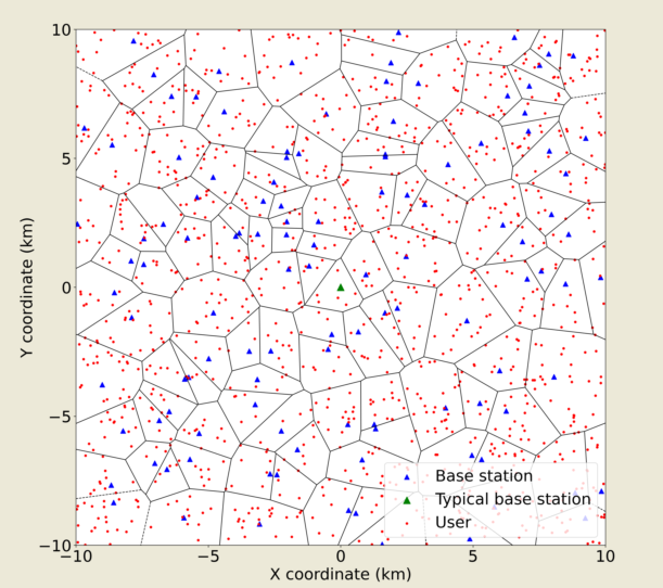
We consider FL in small-cell networks where FC updates global model by combining the locally updated models delivered from users through BSs to FC. The links between BSs and FC are assumed to have infinite capacity with their wired backhaul connections. BSs and users are assumed to be located in the Euclidean plane according to homogeneous PPPs with density and with density , respectively. This assumption makes the network performance analysis significantly more tractable than the traditional grid-based analysis without causing significant error in the network performance [15]. Each user is assumed to be associated with its nearest BS, so that each BS associates with all users located in its Voronoi cell. An example of BS and user deployments are illustrated in Figure 1.
The procedures of FL in small-cell networks can be summarized as follows.
- In the beginning of update round t, FC broadcasts the parameters of global model, , to the distributed users via BSs. Since BSs deliver the same signal , all users are assumed to successfully receive without the interference.
- Each user updates the model parameters on the basis of its local dataset and transmits its local update model to the associated BS. If there are users associated with BS , each associated user transmits its local update model with the bandwidth , where B denotes total bandwidth.
- Each BS averages out the local updates received from its associated users and forwards it to FC.
- FC updates the global model by combining the parameters aggregated from BSs. Then, proceed to update round by starting from step 1 if the convergence condition is not satisfied.
Since the local update report from user to its associated BS suffers from the inter-cell interference and limited communication resources, the step 2 can easily become bottleneck of FL in small-cell networks. For this reason, we focus on the step 2 to facilitate FL in small-cell networks.
According to Slivnyak’s theorem [16], all analysis is conducted for a typical BS located at the origin . The received signal of the typical BS can be represented as
where the index j represents one of users associated with the typical BS, denotes Rayleigh block fading channel gain of user i, denotes link distance between user i and the typical BS, denotes path-loss exponent, denotes the transmit signal of user i, denotes additive noise. All users are assumed to transmit their update with a constant power P. The set consists of the other cell users interfering with the signal reception of the BS. The channel state information (CSI) is assumed to be available only at the BS.
By treating interference as additive noise, the received signal-to-noise-plus-interference (SINR) of a user can be represented as
where follows an exponential distribution with mean P. For the transmission rate u, the conditional coverage probability given users within Voronoi cell is defined as
where denotes a SINR threshold for successful signal reception. Accordingly, for a unit area of model aggregation, the expected number of aggregated bits of locally trained models in a single transmission interval can be represented as
where denotes the coverage probability. Since the time and communication resources for model aggregation decrease with Q, it is required to improve Q for the communication-efficient FL. Based on this understanding, we consider the following optimization problems in two different scenarios.
In the first scenario, for given node densities and , we optimize the transmission rate u to maximize the model aggregation rate Q. Then, the problem is formulated as
In the second scenario, we optimize as well as u to find the minimum required BS deployment for achieving a target aggregation rate . Then, the problem can be formulated as
3. Performance Analysis and Proposed Algorithm
In PPP, the number of users in typical Voronoi cell, K, is dependent on the Voronoi cell size. For given cell size , the number of users K follows Poisson distribution with mean . Accordingly, the probability mass function (PMF) of K can be expanded as
where denotes Gamma function, denotes the probability density function (PDF) of typical Voronoi cell size [17], and is a constant.
where . The number of users in the typical Voronoi cell dependent on the ratio between BS and user densities.
3.1. Coverage Probability
In our uplink system model, the conditional coverage probability can be obtained by modifying the coverage probability expression of the downlink system considered in [15]. The downlink system in [15] has assumed there is at least one user in every Voronoi cell, and therefore all BSs are active . However, such assumption is valid only when the ratio is very low. To derive general expression that is applicable to various BS/user deployments, we relax the low assumption and introduce the active BS density to the coverage probability expression. Furthermore, since our system model assumes each BS serves all its associated users with equal-bandwidth allocation contrary to the downlink system in [15], the SINR threshold becomes a function of random variable K in the coverage probability expression. By additionally taking into account the active BS density and random SINR threshold, the conditional coverage probability (3) can be represented as the following lemma.
Lemma 1.
(Conditional coverage probability). For given transmission rate u and , the conditional coverage probability (3) can be computed as
where
and denotes the density of active BS that contains at least one user in its Voronoi cell.
Based on the independence between BS and user deployments, the deployment of active BS follows PPP with the density
Then, based on (6) and (7), the coverage probability can be represented as
where .
3.2. Coverage Probability in High SNR Regime
In a high SNR regime with a large P, the effect of additive noise becomes negligible compared to the inter-cell interference. Accordingly, the conditional coverage probability (7) simplifies to
Then, the coverage probability (10) can be reduced to
Remark.
In a high SNR regime,
- The coverage probability (12) is dependent on the densities of BSs and users since the probabilities and are functions of . This observation is different with the coverage probability expression presented in [15].
- The conditional coverage probability is an decreasing function of the user density for given and , and it is bounded below by
Special Case:
For a path-loss exponent , the Equation (8) simplifies to
Then, the coverage probability (12) reduces to
Even though the coverage probability is simplified with the assumption , its expression (15) is still complicated to handle. Hence, instead of computing exact coverage probability by taking expectation of over the random variable K, we propose to use its approximation . This approximation will be validated later in the simulation results in Section 5.
The expected number of users in a Voronoi cell can be obtained by
where denotes Stirling number of the second kind. Eventually, for high SNR and , the approximated coverage probability is represented by
4. Transmission Rate and BS Density Optimization
In the first scenario, the optimization problem P1 is equivalent to the problem maximizing the throughput with respect to the transmission rate u. Accordingly, in high SNR regime with , based on (17), the optimization problem can be re-written by
where
Experimentally, the objective is a continuous bell-shaped function with respect to the transmission rate u. Based on this observation, we can see that the solution of the problem P1-1 satisfies the condition as follows
where and . Then, to find the solution that satisfies the condition (19), we can apply the bisection method. Based on Algorithm 1, the solution of the problem P1-1 is obtained as
where , denotes an arbitrary small constant, and denote the minimum and maximum values of transmission rate, respectively.
| Algorithm 1:Bisection Method |
|
In the second scenario, we adopt two-step iterative method to solve the joint optimization problem P2. According to (18), for given transmission rate u, the model aggregation rate Q is a monotonic increasing function of the BS density . Hence, the minimum required BS density for a given u satisfies the constraint with the equality
Based on (21), the density can be obtained by
where is equivalent to the function with a fixed value of u, denotes an arbitrary small constant, and denote the minimum and maximum values of the BS density, respectively. Eventually, the solution of the problem P2 can be obtained by alternately solving the Equations (19) and (21) with Algorithm 1. The process of solving the problem P2 is summarized by Algorithm 2.
| Algorithm 2:Two-Step Iterative Method |
|
5. Simulation Results
In this section, we validate the analysis results on the coverage probability and show the behavior and performance of the proposed algorithm through numerical simulations. All simulation results are obtained with Monte Carlo method by taking average of the results from 2,000 independent deployments in the area [km] and 10,000 independent channel realizations for each deployment. Unless otherwise stated, the simulation environment follows the simulation parameters in Table 1.
Figure 2 shows the coverage probabilities obtained from Monte Carlo simulation and our performance analysis. It is shown that the expressions on the coverage probability (17) and (19) well characterizes the actual coverage probability. In particular, the approximation on the number of in-cell users (19) does not introduce significant error on the coverage probability, and such analysis error becomes negligibly small when . Furthermore, it is confirmed that the coverage probability is a monotonic increasing function of the BS density and a monotonic decreasing function of the transmission rate u.
Figure 3 shows the optimized transmission rates obtained from Monte Carlo simulation and the proposed method (20). It is shown that the optimized transmission rate is a monotonic increasing function of the BS density. Even though there is some error in the analysis result, it is shown to well characterize the effect of BS density on the optimized transmission rate. Furthermore, similar to Figure 2, the analysis error is shown to be negligible when the BS density is low.
Based on the validations on our analysis, Figure 4 shows the results of Algorithm 2 for the joint optimization problem P2 in the second scenario. It is shown that both transmission rate and BS density increase with the performance requirement grows. In addition, if the inter-cell interference becomes severe with the growth in user density, the transmission rate and BS density are shown to be changed so as to increase the coverage probability. It is interesting to note the optimized BS density is nearly saturated at a high user density even though the transmission rate monotonically decreases with the user density. From this observation, we can see that the increase in users is mainly dealt with the transmission rate control.
6. Conclusions
In this paper, we have investigated the wireless model aggregation for FL in small-cell networks where BSs cooperatively aggregate the locally trained model of the edge users. Based on stochastic geometry, we have analyzed the effects of geographic node deployment on the coverage probability and the model aggregation rate. With the approximation on the number of in-cell users of a typical Voronoi cell, we have derived a tractable closed form of the coverage probability in the interference-limited environment. Based on the derived expression, we have proposed two algorithms for maximizing the model aggregation rate and finding the minimum required BS density for achieving the target aggregation rate. The simulation results have confirmed that our analysis result well characterizes the actual performance obtained with Monte Carlo method and the analysis error become negligible when the density ratio is low. Furthermore, our discussions on the minimum required BS density provides insightful information for understanding the model aggregation in small-cell networks, and it can be exploited as a guideline for designing the network facilitating the wireless FL.
Author Contributions
Conceptualization, K.A.N. and J.P.H.; methodology, K.A.N.; software, K.A.N. and Q.A.N.; formal analysis, K.A.N.; data curation, K.A.N. and Q.A.N.; writing—original draft, K.A.N.; writing—review and editing, J.P.H.; visualization, K.A.N.; supervision, J.P.H.; project administration, J.P.H. All authors have read and agreed to the published version of the manuscript.
Funding
This work was supported by the National Research Foundation of Korea (NRF) grant funded by the Korea Government (MSIT) (NRF-2022R1F1A1062930).
Institutional Review Board Statement
Not applicable.
Informed Consent Statement
Not applicable.
Data Availability Statement
All data derived from this study are presented in the article.
Acknowledgments
This work was supported by a Research Grant of Pukyong National University(2021).
Conflicts of Interest
The authors declare no conflict of interest.
References
- McMahan, H.B.; Moore, E.; Ramage, D.; Hampson, S.; Arcas, B.A.y. Communication-Efficient Learning of Deep Networks from Decentralized Data. arXiv 2016, arXiv:1602.05629. [Google Scholar]
- Amiri, M.M.; Gündüz, D. Federated Learning Over Wireless Fading Channels. IEEE Trans. Wireless Commun. 2020, 19, 3546–3557. [Google Scholar] [CrossRef]
- Liu, D.; Zhu, G.; Zhang, J.; Huang, K. Data-Importance Aware User Scheduling for Communication-Efficient Edge Machine Learning. IEEE Trans. Cogn. Commun. Netw. 2021, 7, 265–278. [Google Scholar] [CrossRef]
- Sattler, F.; Wiedemann, S.; Müller, K.-R.; Samek, W. Robust and Communication-Efficient Federated Learning from Non-i.i.d. Data. IEEE Trans. Neural Netw. Learn. Syst. 2020, 31, 3400–3413. [Google Scholar] [CrossRef] [PubMed]
- Yang, K.; Jiang, T.; Shi, Y.; Ding, Z. Federated Learning via Over-the-Air Computation. IEEE Trans. Wireless Commun. 2020, 19, 2022–2035. [Google Scholar] [CrossRef]
- Zhan, Y.; Li, P.; Qu, Z.; Zeng, D.; Guo, S. A Learning-Based Incentive Mechanism for Federated Learning. IEEE Internet Things J. 2020, 7, 6360–6368. [Google Scholar] [CrossRef]
- Tao, Z.; Li, Q. eSGD: Communication Efficient Distributed Deep Learning on the Edge. In Proceedings of the USENIX Workshop on Hot Topics in Edge Computing (HotEdge ’18), Boston, MA, USA, 10 July 2018. [Google Scholar]
- Tao, Z.; Li, Q. CMFL: Mitigating Communication Overhead for Federated Learning. In Proceedings of the 2019 IEEE 39th International Conference on Distributed Computing Systems (ICDCS), Dallas, TX, USA, 7–9 July 2019. [Google Scholar]
- Han, S.; Mao, H.; Dally, W.J. Deep Compression: Compressing Deep Neural Networks with Pruning, Trained Quantization and Huffman Coding. arXiv 2015, arXiv:1510.00149. [Google Scholar]
- Caldas, S.; Konecny, J.; McMahan, H.B.; Talwalkar, A. Expanding the Reach of Federated Learning by Reducing Client Resource Requirements. arXiv 2018, arXiv:1510.00149. [Google Scholar]
- Zhu, G.; Wang, Y.; Huang, K. Broadband Analog Aggregation for Low-Latency Federated Edge Learning. IEEE Trans. Wireless Commun. 2020, 19, 491–506. [Google Scholar] [CrossRef]
- Zeng, Q.; Du, Y.; Huang, K.; Leung, K.K. Energy-Efficient Radio Resource Allocation for Federated Edge Learning. In Proceedings of the 2020 IEEE International Conference on Communications Workshops (ICC Workshops), Dublin, Ireland, 7–11 June 2020. [Google Scholar]
- Lim, W.Y.B.; Nguyen, C.L.; Dinh, T.H.; Jiao, Y.; Liang, Y.-C.; Yang, Q.; Niyato, D.; Miao, C. Federated Learning in Mobile Edge Networks: A Comprehensive Survey. IEEE Commun. Surv. Tutor. 2020, 22, 2031–2063. [Google Scholar] [CrossRef]
- Haenggi, M.; Andrews, J.; Baccelli, F.; Dousse, O.; Franceschetti, M. Stochastic geometry and random graphs for the analysis and design of wireless networks. IEEE J. Sel. Areas Commun. 2009, 27, 1029–1046. [Google Scholar] [CrossRef]
- Andrews, J.; Baccelli, F.; Ganti, R. A Tractable Approach to Coverage and Rate in Cellular Networks. IEEE Trans. Commun. 2011, 59, 3122–3134. [Google Scholar] [CrossRef]
- Yang, H.H.; Liu, Z.; Quek, T.Q.S.; Poor, H.V. Scheduling Policies for Federated Learning in Wireless Networks. IEEE Trans. Commun. 2020, 68, 317–333. [Google Scholar] [CrossRef]
- Singh, S.; Dhillon, H.S.; Andrews, J.G. Offloading in Heterogeneous Networks: Modeling, Analysis, and Design Insights. IEEE Trans. Wireless Commun. 2013, 12, 2484–2497. [Google Scholar] [CrossRef]
- Yu, S.M.; Kim, S. Downlink capacity and base station density in cellular networks. In Proceedings of the 2013 11th International Symposium and Workshops on Modeling and Optimization in Mobile, Ad Hoc and Wireless Networks (WiOpt), Tsukuba, Japan, 13–17 May 2013. [Google Scholar]
- Stoyan, D.; Kendall, W.; Mecke, J. Stochastic Geometry and Its Applications., 2nd ed.; Publisher: John Wiley and Sons, United Kingdom, 1996. [Google Scholar]
- Daley, D.; Jones, D.V. An Introduction to the Theory of Point Processes., 1st ed.; Publisher: Springer, USA, 1988. [Google Scholar]
- ElSawy, H.; Hossain, E.; Haenggi, M. Stochastic Geometry for Modeling, Analysis, and Design of Multi-Tier and Cognitive Cellular Wireless Networks: A Survey. IEEE Commun. Surv. Tutor. 2013, 15, 996–1019. [Google Scholar] [CrossRef]
- Ferenc, J.-S.; Néda, Z. On the size distribution of Poisson Voronoi cells. Physica A: Statistical Mechanics and its Applications. 2007, 385, 518–526. [Google Scholar] [CrossRef]
Figure 1.
Deployments of BSs and users in the area 20×20 [km].
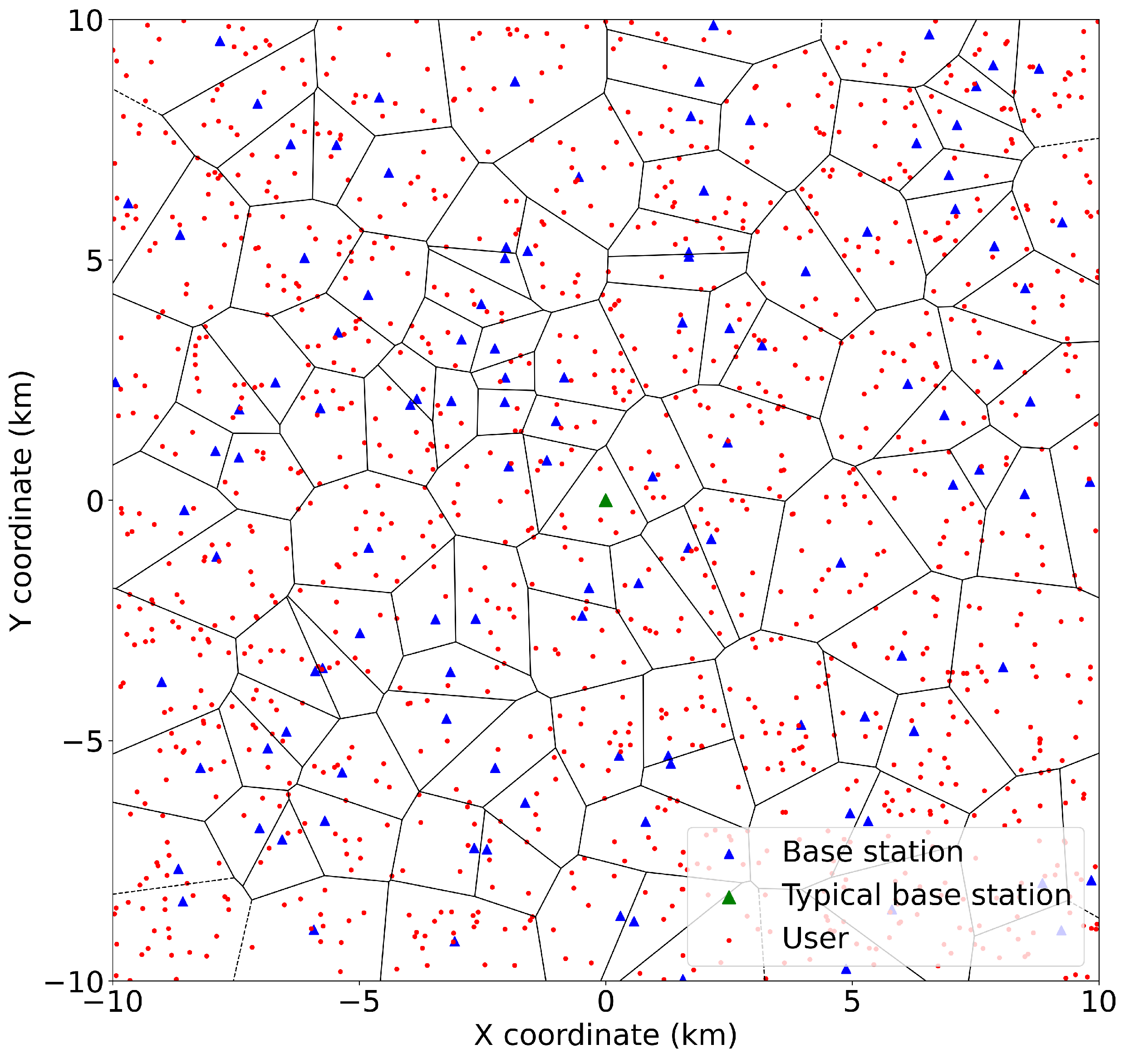
Figure 2.
Coverage probability with respect to .
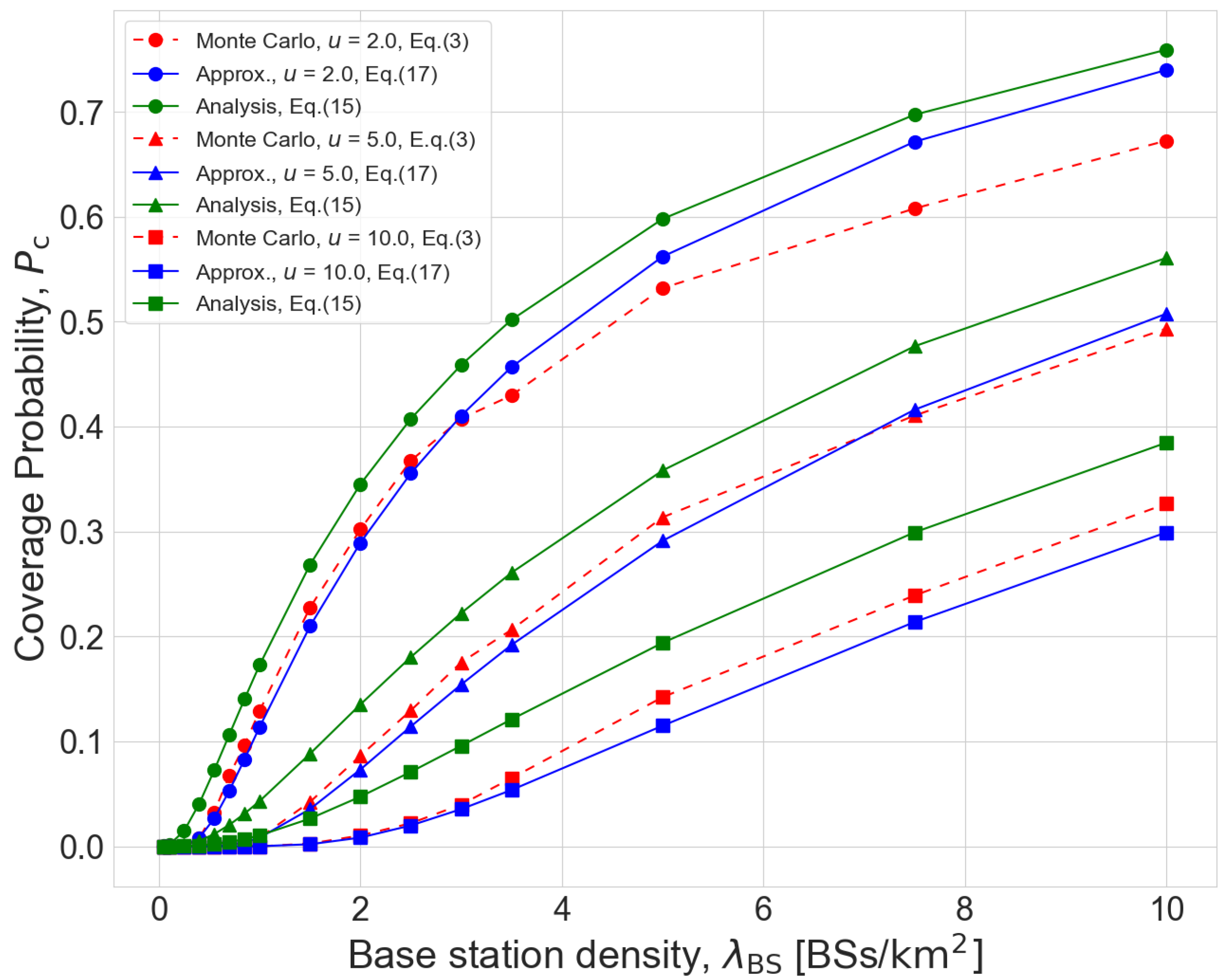
Figure 3.
Optimized transmission rate of the problem P1 for various BS density.
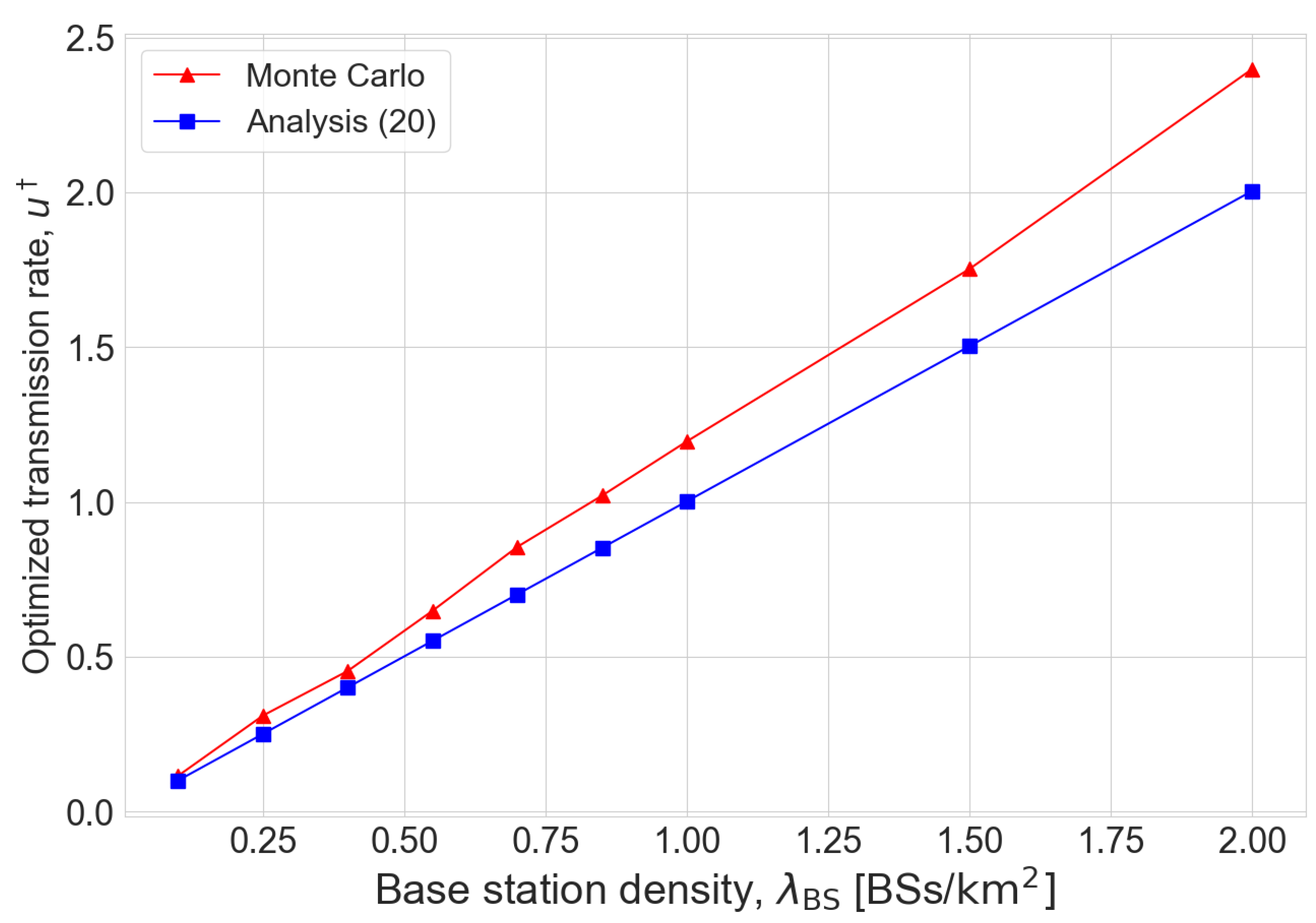
Figure 4.
Solution of joint optimization problem 6 for various user densities. (a) Optimized transmission rate. (b) Optimized BS density.
Figure 4.
Solution of joint optimization problem 6 for various user densities. (a) Optimized transmission rate. (b) Optimized BS density.
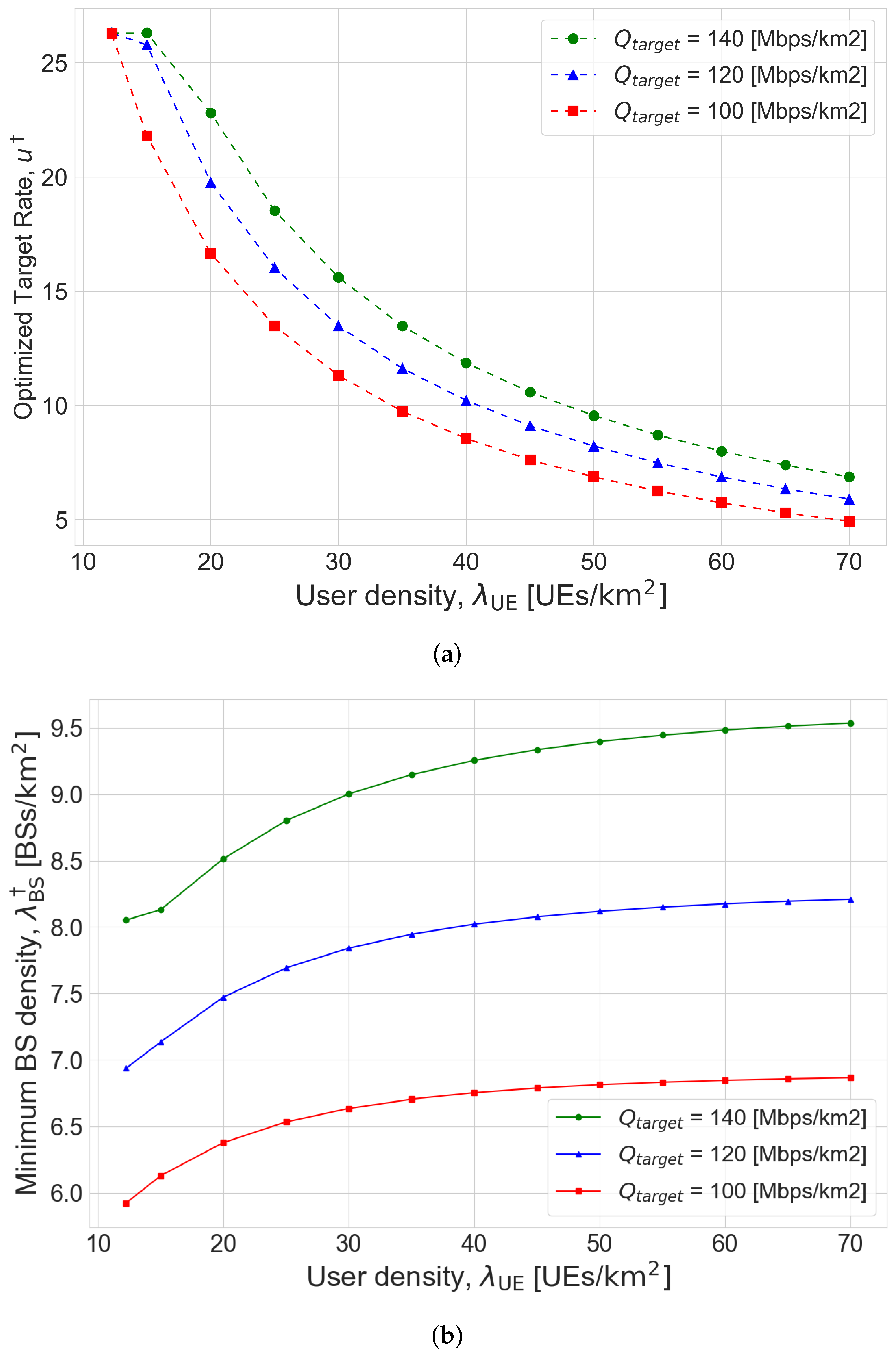

Table 1.
Simulation Parameters.
| Symbol | Description | Value [unit] |
|---|---|---|
| Path-loss exponent | 4 | |
| B | Bandwidth | 20 [MHz] |
| User density | 50 [users/km] | |
| u | Transmission rate | 10 [Mbps] |
| P | Transmit power | 20 [dBm] |
| Additive noise power | [dBm] |
Disclaimer/Publisher’s Note: The statements, opinions and data contained in all publications are solely those of the individual author(s) and contributor(s) and not of MDPI and/or the editor(s). MDPI and/or the editor(s) disclaim responsibility for any injury to people or property resulting from any ideas, methods, instructions or products referred to in the content. |
© 2023 by the authors. Licensee MDPI, Basel, Switzerland. This article is an open access article distributed under the terms and conditions of the Creative Commons Attribution (CC BY) license (http://creativecommons.org/licenses/by/4.0/).
Copyright: This open access article is published under a Creative Commons CC BY 4.0 license, which permit the free download, distribution, and reuse, provided that the author and preprint are cited in any reuse.


