Minor and Major Deformations. Equations of Equilibrium of a Planar Domain with an Angular Cutout of the Boundary

1. Introduction

Large values and gradients of stresses and strains, leading to concentrated stresses and deformations, arise in the corner zones of a structure. The action of forced deformations leading to the finite rupture along the contact between the elements composing the structure, also causes the concentration of stresses, given that the rupture reaches an irregular point, a line on the boundary of the area. The theoretical analysis of the stress-strain state (SSS) of areas with angular cutouts in the boundary under the action of discontinuous forced deformations is reduced to the study of singular solutions to the homogeneous problem of the theory of elasticity that has power-related features [1,2,3,4,5,6,7,8,9,10,11,12,13,14]. Calculation of stress concentration coefficients in the area of the singular solution to the elastic problem makes no sense.

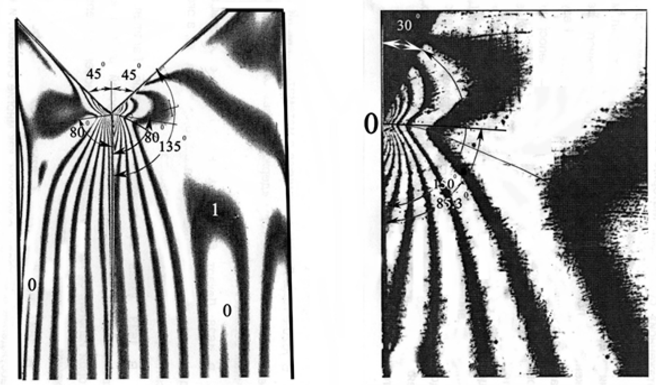
Figure 1 shows interference fringes for a planar model with different angles of cutout in the boundary.

An experimental solution to the elastic problem of forced deformations in the planar domain is illustrated by the case of a composite model of a planar domain with the length of 180 mm and the width of 24 mm. The experimental solution is obtained using methods of deformation defrosting and photo-elasticity [15,16,17,18,19,20].

Temperature-induced deformations $\alpha T{\delta }_{ij}$are made in one part of model ${\Omega }_2$, while the other part ${\Omega }_1$ is not loaded. A spike of temperature deformations along the contact surface of the areas reaches irregular point O (0,0) of the boundary, the vertex of the cutout. Different patterns of fringes are obtained at different angles of the cutout in the boundary (Figure 1).

It is experimentally shown [15,16,17,18,19,20] that substantial deformations and rotations are observed in the zone close to the top of the angular cutout of the boundary area, which corresponds to increasing values of first and second derivatives of displacements along the radius when radii in the neighbourhood of the irregular point of the boundary are small enough. For such areas, it is necessary to consider the plane problem of the elasticity theory, taking into account geometric nonlinearity under the action of forced deformations.

General methods for solving problems in mechanics of deformable solids based on a solution to the nonlinear problem of the elasticity theory were developed in the fundamental works of V. V. Novozhilov [21,22], P.A. Lukash [23], and A.I. Lurie [24], and in works [25,26,27,28,29]. Geometric relations, containing quadratic terms, are used in the nonlinear elasticity theory. Equilibrium equations are formulated as the post-deformation equilibrium of an oblique parallelepiped [21,22,27,28].

Physical equations for the geometrically nonlinear problem of the elasticity theory establish the relationship between stress and deformation components after deformation, so they must be formulated as generalized stresses and nonlinear deformations [21,22,23,24,25,26,27,28]. Therefore, the nonlinear problem of the elasticity theory must be formulated taking into account nonlinear geometric relations and generalized stresses.

In geometrically nonlinear expressions of deformations, different relations may be established between the orders of linear deformations, displacements, rotation angles, and pre-set forced deformations.

The experimental data, obtained using the photo-elasticity method [15,16,17,18,19], show that areas with small deformations and areas with large stress and strain gradients are identified in the area of the angular cutout in the boundary.

The purpose is to analyze the effect of relations of the orders of deformations, rotations, and forced deformations on the form of the equilibrium equation in the polar coordinate system for the V-shaped area under the action of forced temperature-induced deformations with regard to geometric nonlinearity and physical linearity.

Objectives of the work:

1) formulate equilibrium equations for the deformed scheme, obtain equilibrium equations in generalized stresses, deformations for the planar domain, taking into account geometrical nonlinearity and physical linearity.

2) formulate equilibrium equations for the deformed scheme in terms of possible relations of orders of linear deformations, shears, angles of rotation, forced deformations. Analyze the effect of relations of deformation orders on the form of equilibrium equations.

2. Materials and Methods

2.1. Problem Statement

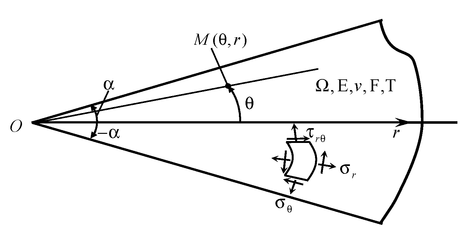
The problem of the elasticity theory is considered for a planar domain with an irregular point on the boundary, or the vertex of an angular cutout of the area. Forced - free temperature deformations $\alpha T{\delta }_{ij}$, where ${\delta }_{ij}$ is the Kronecker symbol, are provided in the planar domain $\Omega$ (Figure 1). In the domain $\Omega ={\Omega }_1\cup {\Omega }_2$, a spike (finite rupture) of forced deformations along the contact line of domains $\Gamma ={\Omega }_1\cap {\Omega }_2$, extending to the vertex of the angular cutout of the area boundary, can be pre-set. For example, deformation discontinuity is triggered, if one of the subdomains ${\Omega }_2$ of the $\Omega ={\Omega }_1\cup {\Omega }_2$ domain is subjected to pre-set temperature-induced deformations $\alpha T{\delta }_{ij}$, while the second subdomain ${\Omega }_1$ is not loaded. Volumetric forces can be pre-set in the planar domain $\Omega$. Concentrated forces are not considered. A homogeneous elastic body is in the 2D deformed state [3,6,29]. Mechanical characteristics include the modulus of elasticity E, Poisson's coefficient $\nu$; they are constant in the $\Omega$ domain. The linear expansion coefficient $\alpha$ in the $\Omega$ domain is constant. Boundary conditions for stresses are homogeneous.

Let’s consider a polar coordinate system with the pole of the polar system O (0,0) at the vertex of the angular cutout of the area boundary. Let the displacement, deformation, and stress functions and their derivatives of an appropriate order be continuous everywhere in the domain $\Omega$, except at the vertex of the angular cutout of the area boundary. If there is a discontinuity of deformations along the contact line of domains $\Gamma ={\Omega }_1\cap {\Omega }_2$, then the continuity conditions for displacements and normal stresses along the contact line of domains are fulfilled. The vertex of the angular cutout of the boundary is removed, and its punctured neighbourhood in domain $\Omega$ is considered.

Figure 1. 2D V-shaped domain $\Omega$.

Figure 1. 2D V-shaped domain $\Omega$.

Different relations for the orders of deformation values are considered depending on the zone of approximation to the irregular point of the boundary to determine different kinds of the solving system for equations of the elastic boundary value problem.

The objective is to formulate equations of equilibrium in the domain $\Omega$, taking into account geometrical nonlinearity and physical linearity.

2.2. Equilibrium Equations

A spatial curvilinear orthogonal coordinate system [17,21,22] ${\alpha }_i$ is considered, i=1,2,3, $\hspace{0.17em}{\overrightarrow{k}}_i\hspace{0.17em}$ are unitary vectors directed toward the positive direction of the ${\alpha }_i$ axes or basis vectors of the domain before the deformation. An infinitesimal element (Figure 1) is selected. This element is limited by six coordinate planes; before deformation this element is a rectangular parallelepiped with edges $H_i\hspace{0.17em}{\overrightarrow{k}}_i\hspace{0.17em}d{\alpha }_i$, where $H_i$ are the Lame parameters. After the deformation, the rectangular parallelepiped transforms into an oblique one with edges $H_i(1+E_{\alpha i})\hspace{0.17em}{\overrightarrow{k}}_i^{*}\hspace{0.17em}d{\alpha }_i$, where $E_{\alpha i}$ are relative elongations along the ${\alpha }_i$ axes after deformation, and $\hspace{0.17em}{\overrightarrow{k}}_i\hspace{0.17em}$ are basis vectors of the domain after the deformation.

Equations of equilibrium of all forces acting on the oblique parallelepiped after the deformation [21,22,24] have the form:

$$\frac{1}{H_1\hspace{0.17em}{H}_2\hspace{0.17em}{H}_3}\left\{\frac{\partial }{\partial {\alpha }_1}(H_2\hspace{0.17em}{H}_3{\overrightarrow{\sigma }}_{n_1}^{*})+\frac{\partial }{\partial {\alpha }_2}(H_3\hspace{0.17em}{H}_1{\overrightarrow{\sigma }}_{n_2}^{*})+\frac{\partial }{\partial {\alpha }_3}(H_1\hspace{0.17em}{H}_2{\overrightarrow{\sigma }}_{n_3}^{*})\right\}+\overrightarrow{F}=0,$$

(1)

where ${\overrightarrow{\sigma }}_{ni}^{*}={\overrightarrow{\sigma }}_{ni}\hspace{0.17em}{S}_i^{*}/S_i$ are generalized stresses on the edges of the oblique parallelepiped, $S_i^{*},\hspace{0.17em}{S}_i$ are the areas of edges of the parallelepiped after and before deformation, $\overrightarrow{F}$ are generalized volume forces after deformation. Having formulated the forces on the edges of the parallelepiped after the deformation in the initial basis of vectors $\hspace{0.17em}{\overrightarrow{k}}_i\hspace{0.17em}$ before the deformation, equations (1) will take the form:

$$\begin{array}{l}(\frac{\partial }{\partial {\alpha }_1}(H_2\hspace{0.17em}{H}_3{s}_{11})+\frac{\partial }{\partial {\alpha }_2}(H_3\hspace{0.17em}{H}_1{s}_{12})+\frac{\partial }{\partial {\alpha }_3}(H_1\hspace{0.17em}{H}_2{s}_{31})+H_3\frac{\partial H_1}{\partial {\alpha }_2}\hspace{0.17em}{s}_{12}+H_2\frac{\partial H_1}{\partial {\alpha }_3}\hspace{0.17em}{s}_{13}-\\ -H_3\frac{\partial H_2}{\partial {\alpha }_1}\hspace{0.17em}{s}_{22}-H_2\frac{\partial H_3}{\partial {\alpha }_1}\hspace{0.17em}{s}_{33}+H_1{H}_2{H}_3{F}_1=0\\ ,\end{array}$$

(2)

$$\begin{array}{l}\frac{\partial }{\partial {\alpha }_1}(H_2\hspace{0.17em}{H}_3{s}_{12})+\frac{\partial }{\partial {\alpha }_2}(H_3\hspace{0.17em}{H}_1{s}_{22})+\frac{\partial }{\partial {\alpha }_3}(H_1\hspace{0.17em}{H}_2{s}_{32})+H_1\frac{\partial H_2}{\partial {\alpha }_3}\hspace{0.17em}{s}_{23}+H_3\frac{\partial H_2}{\partial {\alpha }_1}\hspace{0.17em}{s}_{21}-\\ -H_1\frac{\partial H_3}{\partial {\alpha }_2}\hspace{0.17em}{s}_{33}-H_3\frac{\partial H_1}{\partial {\alpha }_2}\hspace{0.17em}{s}_{11}+H_1{H}_2{H}_3{F}_2=0\end{array},$$

(3)

$$\begin{array}{l}\frac{\partial }{\partial {\alpha }_1}(H_2\hspace{0.17em}{H}_3{s}_{13})+\frac{\partial }{\partial {\alpha }_2}(H_3\hspace{0.17em}{H}_1{s}_{23})+\frac{\partial }{\partial {\alpha }_3}(H_1\hspace{0.17em}{H}_2{s}_{33})+H_3\frac{\partial H_3}{\partial {\alpha }_1}\hspace{0.17em}{s}_{31}+H_1\frac{\partial H_3}{\partial {\alpha }_2}\hspace{0.17em}{s}_{32}-\\ -H_2\frac{\partial H_1}{\partial {\alpha }_3}\hspace{0.17em}{s}_{11}-H_1\frac{\partial H_2}{\partial {\alpha }_3}\hspace{0.17em}{s}_{22}+H_1{H}_2{H}_3{F}_3=0\end{array}.$$

(4)

Here $F_i$ are projections of the generalized volumetric force on directions ${\overrightarrow{k}}_i\hspace{0.17em},i=1,2,3$.

In relations (2), (3), (4) expressions $s_{ij}$ are formulated using generalized stresses ${\sigma }_{ij}^{*}$, deformation parameters $e_{ij}$, rotations ${\omega }_i$:

(5)

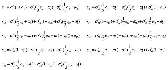
By substituting (5) into equations (2)-(4), one can obtain equations of equilibrium in the curvilinear orthogonal coordinate system ${\alpha }_1\hspace{0.17em},{\alpha }_2\hspace{0.17em},{\alpha }_3$ with account taken of finite deformations for generalized stresses and deformation parameters (5).

We consider a plane problem of the elasticity theory [3,4,6.29] for the state of plane deformation, when the points of the body move in the planes that are perpendicular to the OZ axis:

$$u_1=u_1({\alpha }_1,{\alpha }_2,0),\hspace{0.17em}\hspace{0.17em}{u}_2=u_2({\alpha }_1,{\alpha }_2,0),u_3({\alpha }_1,{\alpha }_2,0)=0.$$

(6)

For the polar coordinate system:

$${\alpha }_1=r, {\alpha }_2=\phi , {\alpha }_3=z.$$

(7)

Lame parameters are:

$$H_1=1,\hspace{0.17em}{H}_2=r,\hspace{0.17em}{H}_3=1$$

(8)

Equilibrium equations (2), (3), (4) will be formulated as follows:

$$\frac{\partial s_{11}}{\partial r}+\frac{1}{r}\frac{\partial s_{21}}{\partial \phi }+\frac{s_{11}-s_{22}}{r}+F_1=0,$$

(9)

$$\frac{1}{r}\frac{\partial s_{22}}{\partial \phi }+\frac{\partial s_{12}}{\partial r}+\frac{s_{12}+s_{21}}{r}+F_2=0,$$

(10)

where relations for generalized stresses (5) in equations (9), (10) will be revised as follows:

$$s_{11}={\sigma }_{11}^{*}(1+e_{11})+{\sigma }_{12}^{*}(\frac{1}{2}{e}_{12}-{\omega }_3),s_{22}={\sigma }_{22}^{*}(1+e_{22})+{\sigma }_{21}^{*}(\frac{1}{2}{e}_{12}+{\omega }_3),$$

(11)

$$s_{12}={\sigma }_{11}^{*}(\frac{1}{2}{e}_{12}+{\omega }_3)+{\sigma }_{12}^{*}(1+e_{22}), s_{21}={\sigma }_{21}^{*}(1+e_{11})+{\sigma }_{22}^{*}(\frac{1}{2}{e}_{12}-{\omega }_3).$$

(12)

Taking into account (11), (12), equations of equilibrium (9), (10) will formulated as follows:

$$\begin{array}{l}\frac{\partial }{\partial r}\left({\sigma }_{11}^{*}(1+e_{11})+{\sigma }_{12}^{*}(\frac{1}{2}{e}_{12}-{\omega }_3)\right)+\frac{1}{r}\frac{\partial }{\partial \phi }\left({\sigma }_{21}^{*}(1+e_{11})+{\sigma }_{22}^{*}(\frac{1}{2}{e}_{12}-{\omega }_3)\right)+\\ +\frac{1}{r}\left[{\sigma }_{11}^{*}(1+e_{11})+{\sigma }_{12}^{*}(\frac{1}{2}{e}_{12}-{\omega }_3)-{\sigma }_{22}^{*}(1+e_{22})-{\sigma }_{21}^{*}(\frac{1}{2}{e}_{12}+{\omega }_3)\right]+F_1=0\end{array},$$

(13)

$$\begin{array}{l}\frac{1}{r}\frac{\partial }{\partial \phi }\left({\sigma }_{21}^{*}(\frac{1}{2}{e}_{12}+{\omega }_3)+{\sigma }_{22}^{*}(1+e_{22})\right)+\frac{\partial }{\partial r}\left({\sigma }_{11}^{*}(\frac{1}{2}{e}_{12}+{\omega }_3)+{\sigma }_{12}^{*}(1+e_{22})\right)+\\ +\frac{1}{r}\left[{\sigma }_{11}^{*}(\frac{1}{2}{e}_{12}+{\omega }_3)+{\sigma }_{12}^{*}(1+e_{22})\hspace{0.17em}+{\sigma }_{21}^{*}(1+e_{11})+{\sigma }_{22}^{*}(\frac{1}{2}{e}_{12}-{\omega }_3)\right]+F_2=0\end{array},$$

(14)

where generalized stresses ${\sigma }_{\mathrm{i}\hspace{0.17em}\mathrm{j}}^{*}$ are related to stresses ${\sigma }_{\mathrm{i}\hspace{0.17em}\mathrm{j}}$ by the following relations at a point in the domain: ${\sigma }_{\mathrm{i}\hspace{0.17em}\mathrm{j}}^{*}=\frac{S_i^{*}}{S_i}{\sigma }_{i\hspace{0.17em}j}\hspace{0.17em},i,j=1,2$.

The form of linear equilibrium equations in generalized stresses in the polar coordinate system of the form (9), (10) coincides with the form of equilibrium equations for minor deformations:

$$\frac{\partial {\sigma }_r}{\partial r}+\frac{1}{r}\frac{\partial {\tau }_{r\theta }}{\partial \theta }+\frac{{\sigma }_r-{\sigma }_{\theta }}{r}+F_1=0,$$

(15)

$$\frac{1}{r}\frac{\partial {\sigma }_{\theta \theta }}{\partial \theta }+\frac{\partial {\tau }_{r\theta }}{\partial r}+\frac{2{\tau }_{r\theta }}{r}+F_2=0.$$

(16)

Let’s formulate equations of equilibrium (13), (14) in deformations.

2.3. Deformation Relations

General deformation relations for the curvilinear orthogonal coordinate system are considered in [21,22,24]. Let’s take advantage of nonlinear relations for deformations in the polar coordinate system [21,30]. The relative elongation $E_{MN}$ at an arbitrary point M of domain $\Omega$ is as follows:

$$E_{MN}=\frac{d{s}^{*}-ds}{ds}=\frac{\left|M^{*}{N}^{*}\right|-\left|MN\right|}{\left|MN\right|},$$

(17)

where ds is the length of the segment MN before the deformation; $d{s}^{*}$ is the length of the segment $M^{*}{N}^{*}$ obtained by moving points M and N after the deformation.

Let’s consider a homogeneous elastic body in the state of plane deformation, for which [3,17,29] is satisfied:

$$u_1=u_1(r,\phi ,0),\hspace{0.17em}\hspace{0.17em}{u}_2=u_2(r,\phi ,0),\hspace{0.17em}\hspace{0.17em}{u}_3=u_3(r,\phi ,0)=0,{\epsilon }_{33}=0, {\epsilon }_{13}={\epsilon }_{31}=0, {\epsilon }_{23}={\epsilon }_{32}=0, e_{13}=e_{31}=0,\hspace{0.17em}{e}_{23}=e_{32}=0,\hspace{0.17em}{e}_{33}=0, e_{33}=0,$$

(18)

$${\sigma }_{13}^{*}={\sigma }_{31}^{*}=0,{\sigma }_{23}^{*}={\sigma }_{32}^{*}=0$$

Deformations in the planar domain $\Omega$ for this unit of elongation (17) will be formulated as follows:

$${\epsilon }_{11}=e_{11}+\frac{1}{2}\left[e_{11}^2+{(\frac{1}{2}{e}_{12}+{\omega }_3)}^2\right], {\epsilon }_{22}=e_{22}+\frac{1}{2}\left[e_{22}^2+{(\frac{1}{2}{e}_{21}-{\omega }_3)}^2\right],$$

(19)

$${\epsilon }_{12}={\epsilon }_{21}=e_{12}+e_{11}(\frac{1}{2}{e}_{12}-{\omega }_3)+e_{22}(\frac{1}{2}{e}_{12}+{\omega }_3).$$

(20)

Here deformation parameters are formulated through displacements $u_1,\hspace{0.17em}{u}_2$ in the polar coordinate system:

$$e_{11}=\frac{\partial u_1}{\partial r}, \hspace{0.17em}{e}_{22}=\frac{1}{r}\frac{\partial u_2}{\partial \phi }+\frac{1}{r}{u}_1, \frac{1}{2}{e}_{12}+{\omega }_3=\frac{\partial u_2}{\partial r},$$

(21)

$$e_{12}=e_{21}=r\frac{\partial }{\partial r}\left(\frac{u_2}{r}\right)+\frac{1}{r}\frac{\partial \hspace{0.17em}{u}_1}{\partial \phi }=\frac{\partial \hspace{0.17em}{u}_2}{\partial r}-\frac{u_2}{r}+\frac{1}{r}\frac{\partial \hspace{0.17em}{u}_1}{\partial \phi }, \frac{1}{2}{e}_{12}-{\omega }_3=\frac{1}{r}\frac{\partial u_1}{\partial \phi }-\frac{u_2}{r}.$$

(22)

Then auxiliary expressions (11), (12) will be reformulated in displacements as follows:

$$s_{11}={\sigma }_{11}^{*}(1+\frac{\partial u_1}{\partial r})+{\sigma }_{12}^{*}(\frac{1}{r}\frac{\partial u_1}{\partial \phi }-\frac{u_2}{r}), s_{22}={\sigma }_{21}^{*}(\frac{\partial u_2}{\partial r})+{\sigma }_{22}^{*}(1+\frac{1}{r}\frac{\partial {\mathrm{u}}_2}{\partial \phi }+\frac{1}{r}{u}_1),$$

(23)

$$s_{12}={\sigma }_{11}^{*}\frac{\partial u_2}{\partial r}+{\sigma }_{12}^{*}(1+\frac{1}{r}\frac{\partial {\mathrm{u}}_2}{\partial \phi }+\frac{1}{r}{u}_1), s_{21}={\sigma }_{21}^{*}(1+\frac{\partial u_1}{\partial r})+{\sigma }_{22}^{*}(\frac{1}{r}\frac{\partial u_1}{\partial \phi }-\frac{u_2}{r})$$

(24)

Taking into account (21), (22), deformations in the polar coordinate system will be formulated as follows in terms of displacements:

$${\epsilon }_{11}=\frac{\partial u_1}{\partial \hspace{0.17em}r}+\frac{1}{2}\left[{\left(\frac{\partial u_1}{\partial \hspace{0.17em}r}\right)}^2+{\left(\frac{\partial u_2}{\partial \hspace{0.17em}r}\right)}^2\right],$$

$${\epsilon }_{22}=\frac{1}{r}\frac{\partial u_2}{\partial \phi }+\frac{u_1}{r}+\frac{1}{2}\left[{\left(\frac{1}{r}\frac{\partial {\mathrm{u}}_2}{\partial \phi }+\frac{u_1}{r}\right)}^2+{\left(\frac{1}{r}\frac{\partial u_1}{\partial \phi }-\frac{u_2}{r}\right)}^2\right],$$

(25)

$${\epsilon }_{12}=\frac{\partial u_2}{\partial r}-\frac{u_2}{r}+\frac{1}{r}\frac{\partial u_1}{\partial \phi }+\frac{\partial u_1}{\partial r}\left(\frac{1}{r}\frac{\partial u_1}{\partial \phi }-\frac{u_2}{r}\right)+\frac{\partial u_2}{\partial r}\left(\frac{1}{r}\frac{\partial u_2}{\partial \phi }+\frac{u_1}{r}\right).$$

Continuity equations for the elastic problem with finite deformations are provided in the general form in [21,22,24].

2.4. Physical Relations

According to [21,22,27,28], it is assumed that the form of relation for generalized stresses and deformatioons is the same as in the Hooke's law in terms of minor deformations. Under the action of forced deformations - temperature deformations, the Dugamel-Neumann dependence will be formulated as follows:

$${\epsilon }_{i\hspace{0.17em}j}=\frac{1+\nu }{E}\left({\sigma }_{ij}^{*}-\frac{\nu }{1+\nu }{s}^{*}{\delta }_{ij}\right)+\alpha T{\delta }_{ij},$$

(26)

where ${\epsilon }_{ij}^0=\frac{1+\nu }{E}\left({\sigma }_{ij}^{*}-\frac{\nu }{1+\nu }{s}^{*}{\delta }_{ij}\right)$is the deformation caused by generalized stresses ${\sigma }_{i\hspace{0.17em}j}^{*}$; ${{\epsilon }^{\prime }}_{ij}^{}=\alpha T{\delta }_{ij}$ are free temperature deformations; E is the modulus of elasticity; $\nu$ is the Poisson's ratio; $s^{*}={\sigma }_{kk}^{*}$ is the sum of normal generalized stresses; $\alpha$ is the linear expansion coefficient; ${\delta }_{ij}$ is the Kronecker symbol.

With regard to (26), generalized stresses are formulated in the polar coordinate system as follows:

$${\sigma }_{11}^{*}=2G{\epsilon }_{11}+\lambda \epsilon -(2\mu +3\lambda )\alpha TЕ,$$

(27)

$${\sigma }_{22}^{*}=2G{\epsilon }_{22}+\lambda \epsilon -(2\mu +3\lambda )\alpha TЕ, {\sigma }_{12}^{*}={\sigma }_{21}^{*}=G{\epsilon }_{12},$$

(28)

Here $2G=2\mu =\frac{E}{1+\nu }$, $\lambda =\frac{\nu E}{(1-2\nu )(1+\nu )}$,$2\mu +3\lambda =\frac{1}{1-2\nu }$, ${\epsilon }_{ij}$ are defined as (19), (20), $\epsilon ={\epsilon }_{11}+{\epsilon }_{22}$.

Let's substitute expressions of stresses (27), (28) into equations of equilibrium (13), (14):

$$\begin{array}{l}\frac{\partial }{\partial r}\left(2G{\epsilon }_{11}+\lambda \epsilon \right)+\frac{1}{r}\frac{\partial }{\partial \phi }G\hspace{0.17em}{\epsilon }_{12}+\frac{1}{r}\left(2G{\epsilon }_{11}+\lambda \epsilon \right)-\frac{1}{r}\left(2G{\epsilon }_{22}+\lambda \epsilon \right)+\\ +\frac{\partial }{\partial r}\left((2G{\epsilon }_{11}+\lambda \epsilon )\hspace{0.17em}{e}_{11}+G\hspace{0.17em}{\epsilon }_{12}(\frac{1}{2}{e}_{12}-{\omega }_3)\right)+\frac{1}{r}\frac{\partial }{\partial \phi }\left(G\hspace{0.17em}{\epsilon }_{12}{e}_{11}+(2G{\epsilon }_{22}+\lambda \epsilon )(\frac{1}{2}{e}_{12}-{\omega }_3)\right)+\\ +\frac{1}{r}\left((2G{\epsilon }_{11}+\lambda \epsilon )e_{11}+G\hspace{0.17em}{\epsilon }_{12}(\frac{1}{2}{e}_{12}-{\omega }_3)\right)-\hspace{0.17em}\frac{1}{r}\left(G\hspace{0.17em}{\epsilon }_{12}(\frac{1}{2}{e}_{12}+{\omega }_3)+(2G{\epsilon }_{22}+\lambda \epsilon )e_{22}\right)+\\ +\frac{(2\mu +3\lambda )\alpha TЕ}{r}(e_{22}-e_{11})-(2\mu +3\lambda )E\frac{\partial }{\partial r}\left(\alpha T(1+e_{11})\right)-\\ -(2\mu +3\lambda )Е\frac{1}{r}\frac{\partial }{\partial \phi }\left(\alpha T(\frac{1}{2}{e}_{12}-{\omega }_3)\right)+F_1=0\end{array},$$

(29)

$$\begin{array}{l}\frac{1}{r}\frac{\partial }{\partial \phi }\left(2G{\epsilon }_{22}+\lambda \epsilon \right)+\frac{\partial }{\partial r}\left(G\hspace{0.17em}{\epsilon }_{12}\right)+\frac{2G}{r}\hspace{0.17em}{\epsilon }_{12}+\frac{1}{r}\frac{\partial }{\partial \phi }\left(G\hspace{0.17em}{\epsilon }_{12}(\frac{1}{2}{e}_{12}+{\omega }_3)+(2G{\epsilon }_{22}+\lambda \epsilon )e_{22})\right)+\\ +\frac{\partial }{\partial r}\left((2G{\epsilon }_{11}+\lambda \epsilon )(\frac{1}{2}{e}_{12}+{\omega }_3)+G\hspace{0.17em}{\epsilon }_{12}{e}_{22})\right)+\frac{1}{r}\hspace{0.17em}\left[(2G{\epsilon }_{11}+\lambda \epsilon )(\frac{1}{2}{e}_{12}+{\omega }_3)+G\hspace{0.17em}{\epsilon }_{12}{e}_{22})\right]\hspace{0.17em}\\ \hspace{0.17em}+\frac{1}{\mathrm{r}}\left[G\hspace{0.17em}{\epsilon }_{12}{e}_{11}+(2G^{*}{\epsilon }_{22}+\lambda \epsilon )(\frac{1}{2}{e}_{12}-{\omega }_3)\right]-\frac{1}{r}(2\mu +3\lambda )\alpha TЕe_{12}-\\ -\frac{1}{r}(2\mu +3\lambda )E(1+e_{22})\frac{\partial }{\partial \phi }\left(\alpha T(1+e_{22})\right)-(2\mu +3\lambda )Е\frac{\partial }{\partial r}\left(\alpha T(\frac{1}{2}{e}_{12}+{\omega }_3)\right)+F_2=0\end{array}.$$

(30)

After the transformations, equilibrium equations (29), (30) will be formulated as follows:

$$\begin{array}{l}\frac{\partial }{\partial r}\left(2G{\epsilon }_{11}+\lambda \epsilon \right)+\frac{1}{r}\frac{\partial }{\partial \phi }G\hspace{0.17em}{\epsilon }_{12}+\frac{1}{r}\left(2G{\epsilon }_{11}+\lambda \epsilon \right)-\frac{1}{r}\left(2G{\epsilon }_{22}+\lambda \epsilon \right)+\\ +\frac{\partial }{\partial r}\left((2G{\epsilon }_{11}+\lambda \epsilon )\hspace{0.17em}{e}_{11}+G\hspace{0.17em}{\epsilon }_{12}(\frac{1}{2}{e}_{12}-{\omega }_3)\right)+\frac{1}{r}\frac{\partial }{\partial \phi }\left(G\hspace{0.17em}{\epsilon }_{12}{e}_{11}+(2G{\epsilon }_{22}+\lambda \epsilon )(\frac{1}{2}{e}_{12}-{\omega }_3)\right)+\\ +\frac{1}{r}\left((2G{\epsilon }_{11}+\lambda \epsilon )e_{11}+G\hspace{0.17em}{\epsilon }_{12}(\frac{1}{2}{e}_{12}-{\omega }_3)\right)-\hspace{0.17em}\frac{1}{r}\left(G\hspace{0.17em}{\epsilon }_{12}(\frac{1}{2}{e}_{12}+{\omega }_3)+(2G{\epsilon }_{22}+\lambda \epsilon )e_{22}\right)+\\ +\frac{(2\mu +3\lambda )\alpha TЕ}{r}(e_{22}-e_{11})-(2\mu +3\lambda )\alpha E\frac{\partial T}{\partial r}-(2\mu +3\lambda )\alpha E\left(T\frac{\partial e_{11}}{\partial r}+e_{11}\frac{\partial T}{\partial r}\right)-\\ -(2\mu +3\lambda )\alpha Е\left(T\frac{1}{r}\frac{\partial }{\partial \phi }(\frac{1}{2}{e}_{12}-{\omega }_3)+(\frac{1}{2}{e}_{12}-{\omega }_3)\frac{1}{r}\frac{\partial T}{\partial \phi }\right)+F_1=0\end{array},$$

(31)

$$\begin{array}{l}\frac{1}{r}\frac{\partial }{\partial \phi }\left(2G{\epsilon }_{22}+\lambda \epsilon \right)+\frac{\partial }{\partial r}\left(G\hspace{0.17em}{\epsilon }_{12}\right)+\frac{2G}{r}\hspace{0.17em}{\epsilon }_{12}+\frac{1}{r}\frac{\partial }{\partial \phi }\left(G\hspace{0.17em}{\epsilon }_{12}(\frac{1}{2}{e}_{12}+{\omega }_3)+(2G{\epsilon }_{22}+\lambda \epsilon )e_{22})\right)+\\ +\frac{\partial }{\partial r}\left((2G{\epsilon }_{11}+\lambda \epsilon )(\frac{1}{2}{e}_{12}+{\omega }_3)+G\hspace{0.17em}{\epsilon }_{12}{e}_{22})\right)+\frac{1}{r}\hspace{0.17em}\left[(2G{\epsilon }_{11}+\lambda \epsilon )(\frac{1}{2}{e}_{12}+{\omega }_3)+G\hspace{0.17em}{\epsilon }_{12}{e}_{22})\right]\hspace{0.17em}\\ +\frac{1}{\mathrm{r}}\left[G\hspace{0.17em}{\epsilon }_{12}{e}_{11}+(2G^{*}{\epsilon }_{22}+\lambda \epsilon )(\frac{1}{2}{e}_{12}-{\omega }_3)\right]-\frac{1}{r}(2\mu +3\lambda )\alpha TЕe_{12}-\frac{1}{r}(2\mu +3\lambda )\alpha E(1+e_{22})\frac{\partial T}{\partial \phi }\\ -(2\mu +3\lambda )\alpha Е(\frac{1}{2}{e}_{12}+{\omega }_3)\frac{\partial T}{\partial r}-\frac{1}{r}(2\mu +3\lambda )\alpha ET\frac{\partial e_{22}}{\partial \phi }-(2\mu +3\lambda )\alpha TЕ\frac{\partial }{\partial r}(\frac{1}{2}{e}_{12}+{\omega }_3)+F_2=0\end{array}$$

(32)

Equilibrium Equations (29), (30) or (31), (32) are formulated for the deformed scheme with account taken of geometrical nonlinearity (19), (20) and physical linearity (27), (28) under the action of forced deformations and volumetric forces.

2.5. Relations of Orders for Deformations

The classification of geometrically nonlinear solutions of elasticity theory problems was proposed by V.V. Novozhilov [21,22,31] and is discussed in [23,24,27,28]. Let’s consider deformations (19), (20) and equations of equilibrium (29), (30) depending on the orders of elastic body deformation for the state of plane deformation by using the classification developed by V.V. Novozhilov [21,22].

Let's consider the following options:

Option I - elongations, shears, and rotations are small and small compared to unity,

Option II - elongations, shears, rotations are not small compared to unity.

Displacements in the zone of the angular cutout of the boundary are small and continuous.

According to [21,22,31], angles of rotations, elongations and shears enter into deformation relations (19), (20) in the following ways:

1) parameters $e_{11},\hspace{0.17em}{e}_{22},\hspace{0.17em}{e}_{12}$ are linear,

2) products of parameters $e_{11}\hspace{0.17em}{e}_{12},\hspace{0.17em}\hspace{0.17em}{e}_{22}\hspace{0.17em}{e}_{12},\hspace{0.17em}\hspace{0.17em}{e}_{11}^2\hspace{0.17em},\hspace{0.17em}\hspace{0.17em}{e}_{22}^2,\hspace{0.17em}\hspace{0.17em}\hspace{0.17em}{e}_{12}^2,\hspace{0.17em}\hspace{0.17em}{e}_{21}^2$,

3) square of the rotation parameter ${\omega }_3^2$ ,

4) products of parameters $e_{12}\cdot {\omega }_3$, $e_{21}\hspace{0.17em}\cdot {\omega }_3$.

Let’s consider option I.

Case A) – the value of rotation ${\omega }_3$ is small and of the same or higher order of smallness than $e_{\mathrm{i}\hspace{0.17em}\mathrm{j}}\hspace{0.17em}$.

Case B) - values of deformation parameters $e_{\mathrm{i}\hspace{0.17em}\mathrm{j}}\hspace{0.17em}$are small and of the same or higher order of smallness than squares of rotation ${\omega }_3^2$.

Case A).

Let’s consider small parameters $e_{\mathrm{i}\hspace{0.17em}\mathrm{j}}\hspace{0.17em}$ and small rotations ${\omega }_3$, that are smaller than unity: $e_{ij}^2=o(e_{ij})$, ${\omega }_3^2=o({\omega }_3)$ or ${\omega }_3^2$<<$e_{\mathrm{i}\hspace{0.17em}\mathrm{j}}\hspace{0.17em}$ We take values of the first order of smallness $e_{\mathrm{i}\hspace{0.17em}\mathrm{j}}\hspace{0.17em}$, ${\omega }_3$ as initial values.

The value of rotation ${\omega }_3$ is small and of the same or higher order of smallness than $e_{\mathrm{i}\hspace{0.17em}\mathrm{j}}\hspace{0.17em}$, so $e_{\mathrm{i}\hspace{0.17em}\mathrm{j}}\hspace{0.17em}{\omega }_3=o({\omega }_3)=o(e_{\mathrm{i}\hspace{0.17em}\mathrm{j}})$.

$${\epsilon }_{11}=e_{11}+o(e_{11})\approx e_{11}=\frac{\partial u_1}{\partial \hspace{0.17em}r}, {\epsilon }_{22}=e_{22}+o(e_{22})\approx e_{22}=\frac{1}{r}\frac{\partial u_2}{\partial \phi }+\frac{u_1}{r},$$

(33)

$${\epsilon }_{12}={\epsilon }_{21}=e_{12}+o(e_{12})\approx e_{12}=\frac{\partial u_2}{\partial r}-\frac{u_2}{r}+\frac{1}{r}\frac{\partial u_1}{\partial \phi }.$$

(34)

For these orders of smallness of deformation values, in the absence of volumetric forces equations of equilibrium (29), (30) are formulated as follows:

$$\begin{array}{l}\frac{\partial }{\partial r}\left(2G{\epsilon }_{11}+\lambda \epsilon \right)+\frac{1}{r}\frac{\partial }{\partial \phi }\left(G{\epsilon }_{12}\right)+\frac{2G}{r}({\epsilon }_{11}-{\epsilon }_{22})+\frac{(2\mu +3\lambda )E}{r}\alpha T(e_{22}-e_{11})\\ -(2\mu +3\lambda )E\frac{\partial }{\partial r}\left(\alpha T(1+e_{11})\right)-\frac{(2\mu +3\lambda )E}{r}\frac{\partial }{\partial \phi }\left(\alpha T(\frac{1}{2}{e}_{12}-{\omega }_3)\right)=0\end{array},$$

(35)

$$\begin{array}{l}\frac{1}{r}\frac{\partial }{\partial \phi }\left(2G{\epsilon }_{22}+\lambda \epsilon \right)+\frac{\partial }{\partial r}\left(G{\epsilon }_{12}\right)+\frac{2G}{r}{\epsilon }_{12}-\frac{(2\mu +3\lambda )\alpha TЕ}{r}{\epsilon }_{12}-\\ -\frac{(2\mu +3\lambda )Е}{r}\frac{\partial }{\partial \phi }\left(\alpha T(1+{\epsilon }_{22})\right)\hspace{0.17em}-(2\mu +3\lambda )E\frac{\partial }{\partial r}\left(\alpha T(\frac{1}{2}{\epsilon }_{12}+{\omega }_3)\right)=0\end{array}.$$

(36)

Taking into account linear deformations (33), (34), equations (35), (36) will be formulated as follows:

$$\begin{array}{l}\frac{\partial }{\partial r}\left(2G{\mathrm{e}}_{11}+\lambda ({\mathrm{e}}_{11}+{\mathrm{e}}_{22}\right)+\frac{1}{r}\frac{\partial }{\partial \phi }\left(G{e}_{12}\right)+\frac{2G}{r}(e_{11}-e_{22})+\frac{(2\mu +3\lambda )E}{r}\alpha T(e_{22}-e_{11})-\\ -(2\mu +3\lambda )E\frac{\partial }{\partial r}\left(\alpha T(1+e_{11})\right)-\frac{(2\mu +3\lambda )E}{r}\frac{\partial }{\partial \phi }\left(\alpha T(\frac{1}{2}{e}_{12}-{\omega }_3)\right)=0\end{array},$$

(37)

$$\begin{array}{l}\frac{1}{r}\frac{\partial }{\partial \phi }\left(2G{e}_{22}+\lambda (e_{11}+e_{22}\right)+\frac{\partial }{\partial r}\left(G{e}_{12}\right)+\frac{2G}{r}{e}_{12}-\frac{(2\mu +3\lambda )\alpha TЕ}{r}{e}_{12}-\\ -\frac{(2\mu +3\lambda )Е}{r}\frac{\partial }{\partial \phi }\left(\alpha T(1+e_{22})\right)\hspace{0.17em}-(2\mu +3\lambda )E\frac{\partial }{\partial r}\left(\alpha T(\frac{1}{2}{e}_{12}+{\omega }_3)\right)=0\end{array}.$$

(38)

Case A1).

Let the temperature deformations $\alpha T{\delta }_{ij}$ have the same order of smallness as $e_{\mathrm{i}\hspace{0.17em}\mathrm{j}}\hspace{0.17em}$ or a higher order of smallness than $e_{\mathrm{i}\hspace{0.17em}\mathrm{j}}\hspace{0.17em}$, i.e. $\alpha T{\epsilon }_{ij}=o({\epsilon }_{ij}),\alpha T{\omega }_3=o({\omega }_3)$, then equations (35), (36) are reformulated as follows:

$$\frac{\partial }{\partial r}\left(2G{\epsilon }_{11}+\lambda \epsilon \right)+\frac{1}{r}\frac{\partial }{\partial \phi }\left(G{\epsilon }_{12}\right)+\frac{2G}{r}({\epsilon }_{11}-{\epsilon }_{22})-(2\mu +3\lambda )\alpha E\frac{\partial T}{\partial r}=0,$$

(39)

$$\frac{1}{r}\frac{\partial }{\partial \phi }\left(2G{\epsilon }_{22}+\lambda \epsilon \right)+\frac{\partial }{\partial r}\left(G{\epsilon }_{12}\right)+\frac{2G}{r}{\epsilon }_{12}-\frac{(2\mu +3\lambda )\alpha Е}{r}\frac{\partial T}{\partial \phi }\hspace{0.17em}=0.$$

(40)

If deformations (33), (34) are taken into account, equations (39), (40) will be formulated as follows:

$$\frac{\partial }{\partial r}\left(2G{e}_{11}+\lambda (e_{11}+e_{22})\right)+\frac{1}{r}\frac{\partial }{\partial \phi }\left(G{e}_{12}\right)+\frac{2G}{r}(e_{11}-e_{22})-(2\mu +3\lambda )E\frac{\partial }{\partial r}\left(\alpha T\right)=0,$$

(41)

$$\frac{1}{r}\frac{\partial }{\partial \phi }\left(2G{e}_{22}+\lambda (e_{11}+e_{22}\right)+\frac{\partial }{\partial r}\left(G{e}_{12}\right)+\frac{2G}{r}{e}_{12}-\frac{(2\mu +3\lambda )Е}{r}\frac{\partial }{\partial \phi }\left(\alpha T\right)\hspace{0.17em}=0.$$

(42)

CaseА2).

If the temperature in one area is constant and the other area is free of loads, then for Case A1) we obtain the following homogeneous system of equations:

$$\frac{\partial }{\partial r}\left(2G{e}_{11}+\lambda (e_{11}+e_{22})\right)+\frac{1}{r}\frac{\partial }{\partial \phi }\left(G{e}_{12}\right)+\frac{2G}{r}(e_{11}-e_{22})=0,$$

(43)

$$\frac{1}{r}\frac{\partial }{\partial \phi }\left(2G{e}_{22}+\lambda (e_{11}+e_{22}\right)+\frac{\partial }{\partial r}\left(G{e}_{12}\right)+\frac{2G}{r}{e}_{12}=0.$$

(44)

Case B).

Deformation parameters $e_{\mathrm{i}\hspace{0.17em}\mathrm{j}}\hspace{0.17em}$ are small and of the same order of smallness as ${\omega }_3^2$: $e_{\mathrm{i}\hspace{0.17em}\mathrm{j}}\hspace{0.17em}\sim {\omega }_3^2$, or of a higher order of smallness than ${\omega }_3^2$:$e_{\mathrm{i}\hspace{0.17em}\mathrm{j}}\hspace{0.17em}$<<${\omega }_3^2$ or $e_{\mathrm{i}\hspace{0.17em}\mathrm{j}}\hspace{0.17em}=o({\omega }_3^2)$.

Deformation relations (19), (20) will be formulated as follows:

$${\epsilon }_{11}=e_{11}+\frac{1}{2}{({\omega }_3)}^2,{\epsilon }_{22}=e_{22}+\frac{1}{2}{({\omega }_3)}^2,{\epsilon }_{12}={\epsilon }_{21}=e_{12},\epsilon =e_{11}+e_{22}+{\omega }_3^2.$$

(45)

In this case, equilibrium equations (31), (32) will be formulated as follows:

$$\begin{array}{l}\frac{\partial }{ \partial r}\left(2G(e_{11}+\frac{1}{2}{\omega }_3^2)+\lambda (e_{11}+e_{22}+{\omega }_3^2\right)+\frac{1}{r}\frac{\partial }{\partial \phi }\left(G{e}_{12}\right)+\frac{(2\mu +3\lambda )E}{r}\alpha T(e_{22}-e_{11})-\\ -(2\mu +3\lambda )E\frac{\partial }{\partial r}\left(\alpha T(1+e_{11})\right)-\frac{(2\mu +3\lambda )E}{r}\frac{\partial }{\partial \phi }\left(\alpha T(\frac{1}{2}{e}_{12}-{\omega }_3)\right)=0\end{array},$$

(46)

$$\begin{array}{l}\frac{1}{r}\frac{\partial }{\partial \phi }\left[2G(e_{22}+\frac{1}{2}\hspace{0.17em}{\omega }_3^2)+\lambda (e_{11}+e_{22}+{\omega }_3^2)\right]+\frac{\partial }{\partial r}\left(G{e}_{12}\right)+\frac{2G}{r}{e}_{12}-\\ -\frac{(2\mu +3\lambda )Е}{r}\frac{\partial }{\partial \phi }\left(\alpha T(1+e_{22})\right)\hspace{0.17em}-\frac{(2\mu +3\lambda )\alpha TЕ}{r}{e}_{12}=0\end{array}.$$

(47)

Case B1).

Let the temperature deformations $\alpha T{\delta }_{ij}$ have the same order of smallness as ${\omega }_3$, i.e., $\alpha T\sim {\omega }_3$, then the value $\alpha T{\omega }_3$ has the order ${\omega }_3^2$, which should be taken into account. In this case equations (46), (47) will be formulated as follows:

$$\begin{array}{l}\frac{\partial }{\partial r}\left(2G(e_{11}+\frac{1}{2}{\omega }_3^2)+\lambda (e_{11}+e_{22}+{\omega }_3^2\right)+\frac{1}{r}\frac{\partial }{\partial \phi }\left(G{e}_{12}\right)-\\ -(2\mu +3\lambda )E\frac{\partial }{\partial r}\alpha T+\frac{(2\mu +3\lambda )E}{r}\frac{\partial }{\partial \phi }\left(\alpha T{\omega }_3\right)=0\end{array},$$

(48)

$$\begin{array}{l}\frac{1}{r}\frac{\partial }{\partial \phi }\left[2G(e_{22}+\frac{1}{2}\hspace{0.17em}{\omega }_3^2)+\lambda (e_{11}+e_{22}+{\omega }_3^2)\right]+\frac{\partial }{\partial r}\left(G{e}_{12}\right)+\frac{2G}{r}{e}_{12}-\\ -\frac{(2\mu +3\lambda )Е}{r}\frac{\partial }{\partial \phi }\left(\alpha T\right)\hspace{0.17em}=0\end{array}.$$

(49)

Case B2).

Let the temperature deformations $\alpha T{\delta }_{ij}$ have a higher order of smallness than ${\omega }_3^2$, then equations (48), (49) will be formulated as follows:

$$\frac{\partial }{\partial r}\left(2G(e_{11}+\frac{1}{2}{\omega }_3^2)+\lambda (e_{11}+e_{22}+{\omega }_3^2\right)+\frac{1}{r}\frac{\partial }{\partial \phi }\left(G{e}_{12}\right)-(2\mu +3\lambda )E\frac{\partial }{\partial r}\alpha T=0.$$

(50)

$$\begin{array}{l}\frac{1}{r}\frac{\partial }{\partial \phi }\left[2G(e_{22}+\frac{1}{2}\hspace{0.17em}{\omega }_3^2)+\lambda (e_{11}+e_{22}+{\omega }_3^2)\right]+\frac{\partial }{\partial r}\left(G{e}_{12}\right)+\frac{2G}{r}{e}_{12}-\\ -\frac{(2\mu +3\lambda )Е}{r}\frac{\partial }{\partial \phi }\left(\alpha T\right)\hspace{0.17em}=0\end{array}.$$

(51)

If the temperature in one area is constant, the other area is free of loads, then the following homogeneous system of equations is obtained:

$$\frac{\partial }{\partial r}\left(2G(e_{11}+\frac{1}{2}{\omega }_3^2)+\lambda (e_{11}+e_{22}+{\omega }_3^2\right)+\frac{1}{r}\frac{\partial }{\partial \phi }\left(G{e}_{12}\right)=0,$$

(52)

$$\frac{1}{r}\frac{\partial }{\partial \phi }\left[2G(e_{22}+\frac{1}{2}\hspace{0.17em}{\omega }_3^2)+\lambda (e_{11}+e_{22}+{\omega }_3^2)\right]+\frac{\partial }{\partial r}\left(G{e}_{12}\right)+\frac{2G}{r}{e}_{12}=0.$$

(52)

CaseС).

Displacements $u_1,\hspace{0.17em}{u}_2$ in the area nearing the vertex of the angular area have a power form: $u_i=r^{\lambda }{f}_i(\theta ),\lambda \in [0,\hspace{0.17em}0.5]$, the first derivatives of the displacement function along the radius are of order $r^{\lambda -1}=\frac{1}{r^{1-\lambda }}$. The value of $\frac{1}{r^{1-\lambda }}$ increases for small radii $r\to 0$. Thus, at $\lambda \in (0,\hspace{0.17em}0.5)$ the value is $\frac{1}{r^{1-\lambda }}\in \left[\frac{1}{\sqrt{r}},\frac{1}{r}\right]$, and the square of the value is $\frac{1}{r^{2-2\lambda }}\in \left[\frac{1}{r},\frac{1}{r^2}\right]$, so the nonlinear part of the deformation relations, which takes into account the squares of deformations and rotations (19), (20) at small radii is significant in value compared to the linear part of the deformation relations.

For such a neighbourhood, excluding the very vertex of the angular cutout of the boundary, without taking into account the nonlinear part of the deformation relations, stresses and strains of order $r^{\lambda -1}$, i.e., ${\sigma }_{\mathrm{i}\hspace{0.17em}\mathrm{j}},\hspace{0.17em}{\epsilon }_{\mathrm{i}\hspace{0.17em}\mathrm{j}}\sim r^{\lambda -1}f(\phi )$, $\lambda \in (0,\hspace{0.17em}0.5)$, are observed.

For such a neighbourhood, excluding the very vertex of the angular cutout of the boundary, we assume the deformations and rotations to be of the same order of variation along the radius. Deformations $e_{\mathrm{i}\hspace{0.17em}\mathrm{j}}\hspace{0.17em}$ have a higher order of smallness than $e_{i\hspace{0.17em}j}^2\hspace{0.17em}$: $e_{\mathrm{i}\hspace{0.17em}\mathrm{j}}\hspace{0.17em}=o(e_{i\hspace{0.17em}j}^2)$, rotations ${\omega }_i$ are of the same order as deformations $e_{\mathrm{i}\hspace{0.17em}\mathrm{j}}\hspace{0.17em}$, i.e. $\omega \sim r^{\lambda -1}$, ${\omega }_{\mathrm{i}}\hspace{0.17em}=o({\omega }_i^2)$, with the radius being sufficiently small.

Deformations (19), (20), taking into account relations $e_{\mathrm{i}\hspace{0.17em}\mathrm{j}}\hspace{0.17em}=o(e_{i\hspace{0.17em}j}^2)$, ${\omega }_i\hspace{0.17em}=o({\omega }_i^2)$, will be formulated as follows:

$${\epsilon }_{22}\approx \frac{1}{2}\left[e_{22}^2+{(\frac{1}{2}{e}_{21}-{\omega }_3)}^2\right], {\epsilon }_{11}\approx \frac{1}{2}\left[e_{11}^2+{(\frac{1}{2}{e}_{12}+{\omega }_3)}^2\right],$$

(53)

$${\epsilon }_{12}={\epsilon }_{21}\approx e_{11}(\frac{1}{2}{e}_{12}-{\omega }_3)+e_{22}(\frac{1}{2}{e}_{12}+{\omega }_3), \epsilon \approx \frac{1}{2}\left[e_{11}^2+e_{22}^2+\frac{1}{2}{e}_{12}^2+2{\omega }_3^2\right].$$

(54)

Let the deformations and rotations be limited to the corresponding area of the angular cutout of the boundary and have the same second order of variation, taken as the initial one. We disregard values of the deformation parameters above the third order as those that are leading to a substantial increase in the potential energy of deformation.

The first equation of general equilibrium (29) in the absence of volumetric forces:

$$\begin{array}{l}\frac{\partial }{\partial r}\left(\left(2G{\epsilon }_{11}+\lambda \epsilon -(2\mu +3\lambda )\alpha TЕ\right)(1+e_{11})+\left(G{\epsilon }_{12}\right)(\frac{1}{2}{e}_{12}-{\omega }_3)\right)+\\ +\frac{1}{r}\frac{\partial }{\partial \phi }\left(\left(G{\epsilon }_{12}\right)(1+e_{11})+\left(2G{\epsilon }_{22}+\lambda \epsilon -(2\mu +3\lambda )\alpha TЕ\right)(\frac{1}{2}{e}_{12}-{\omega }_3)\right)+\\ +\frac{1}{r}\left(\left(2G{\epsilon }_{11}+\lambda \epsilon -(2\mu +3\lambda )\alpha TЕ\right)(1+e_{11})+\left(G{\epsilon }_{12}\right)(\frac{1}{2}{e}_{12}-{\omega }_3)\right)-\\ -\frac{1}{r}\left(\left(G{\epsilon }_{12}\right)(\frac{1}{2}{e}_{12}+{\omega }_3)+\left(2G{\epsilon }_{22}+\lambda \epsilon -(2\mu +3\lambda )\alpha TЕ\right)(1+e_{22})\right)=0\end{array}$$

(55)

is reformulated for the pre-set relations of deformation orders (53), (54) of case C in the form:

$$\begin{array}{l}\frac{\partial }{\partial r}\left(2G{\epsilon }_{11}+\lambda \epsilon \right)+\frac{1}{r}\frac{\partial }{\partial \phi }\left(G{\epsilon }_{12}\right)+\frac{1}{r}2G({\epsilon }_{11}-{\epsilon }_{22})\\ -(2\mu +3\lambda )E\frac{\partial }{\partial r}\alpha T(1+{\mathrm{e}}_{11})-(2\mu +3\lambda )Е\frac{1}{r}\frac{\partial }{\partial \phi }\alpha T(\frac{1}{2}{e}_{12}-{\omega }_3)+\\ -\frac{1}{r}(2\mu +3\lambda )\alpha TЕ(1+e_{11})+\frac{1}{r}(2\mu +3\lambda )\alpha TЕ(1+e_{22})=0\end{array}.$$

(56)

The second equation of equilibrium in the general form (30) in the absence of volumetric forces:

$$\begin{array}{l}\frac{1}{r}\frac{\partial }{\partial \phi }\left(\left(G{\epsilon }_{12}\right)(\frac{1}{2}{e}_{12}+{\omega }_3)+\left(2G{\epsilon }_{22}+\lambda \epsilon -(2\mu +3\lambda )\alpha TЕ\right)(1+e_{22})\right)+\\ +\frac{\partial }{\partial r}\left(\left(2G{\epsilon }_{11}+\lambda \epsilon -(2\mu +3\lambda )\alpha TЕ\right)(\frac{1}{2}{e}_{12}+{\omega }_3)+\left(G{\epsilon }_{12}\right)(1+e_{22})\right)+\\ +\frac{1}{r}\left(\left(2G{\epsilon }_{11}+\lambda \epsilon -(2\mu +3\lambda )\alpha TЕ\right)(\frac{1}{2}{e}_{12}+{\omega }_3)+\left(G{\epsilon }_{12}\right)(1+e_{22})\right)+\\ +\frac{1}{r}\left(\left(G{\epsilon }_{12}\right)(1+e_{11})+\left(2G{\epsilon }_{22}+\lambda \epsilon -(2\mu +3\lambda )\alpha TЕ\right)(\frac{1}{2}{e}_{12}-{\omega }_2)\right)=0\end{array}$$

(57)

after transformations for these relations of deformations order (53), (54) of case C will be formulated as follows:

$$\begin{array}{l}\frac{1}{r}\frac{\partial }{\partial \phi }(2G{\epsilon }_{22}+\lambda \epsilon )+\frac{\partial }{\partial r}\left(G{\epsilon }_{12}\right)+\frac{2G}{r}{\epsilon }_{12}-\frac{1}{r}(2\mu +3\lambda )\alpha TЕ\hspace{0.17em}{e}_{12}-\\ -(2\mu +3\lambda )Е\frac{1}{r}\frac{\partial }{\partial \phi }\alpha T(1+e_{22})-(2\mu +3\lambda )Е\frac{\partial }{\partial r}\alpha T(\frac{1}{2}{e}_{12}+{\omega }_3)=0\end{array}.$$

(58)

Please mind that the form of equilibrium equations (56), (58) for major deformations of the form (53), (54) coincides with the form of equilibrium equations (35), (36) for minor deformations (33), (34), the difference being determined by substituting the corresponding deformations (53), (54) or (33), (34).

CaseС1)

Let the temperature deformations $\alpha T{\delta }_{ij}$ have the same order of variation as $e_{\mathrm{i}\hspace{0.17em}\mathrm{j}}\hspace{0.17em}$,${\omega }_3$. We take the second order of variation of the deformation parameters as the initial one in the corresponding neighbourhood of the vertex of the angular cutout of the boundary in case of sufficiently small radii: i.e., $\alpha T{\delta }_{ij}=o(e_{ij}^2),\alpha T=o({\omega }_3^2)$. Equations (56), (58) are reformulated as follows:

$$\begin{array}{l}\frac{\partial }{\partial r}\left(2G{\epsilon }_{11}+\lambda \epsilon \right)+\frac{1}{r}\frac{\partial }{\partial \phi }\left(G{\epsilon }_{12}\right)+\frac{1}{r}2G({\epsilon }_{11}-{\epsilon }_{22})+\frac{1}{r}(2\mu +3\lambda )\alpha TЕ(e_{22}-e_{11})-\\ -(2\mu +3\lambda )E\frac{\partial }{\partial r}\alpha T{\mathrm{e}}_{11}-(2\mu +3\lambda )Е\frac{1}{r}\frac{\partial }{\partial \phi }\alpha T(\frac{1}{2}{e}_{12}-{\omega }_3)=0\end{array},$$

(59)

$$\begin{array}{l}\frac{1}{r}\frac{\partial }{\partial \phi }(2G{\epsilon }_{22}+\lambda \epsilon )+\frac{\partial }{\partial r}\left(G{\epsilon }_{12}\right)+\frac{2G}{r}{\epsilon }_{12}-\frac{1}{r}(2\mu +3\lambda )\alpha TЕ\hspace{0.17em}{e}_{12}-\\ -(2\mu +3\lambda )Е\frac{1}{r}\frac{\partial }{\partial \phi }\alpha T{e}_{22})-(2\mu +3\lambda )Е\frac{\partial }{\partial r}\alpha T(\frac{1}{2}{e}_{12}+{\omega }_3)=0\end{array}$$

(60)

where ${\epsilon }_{ij}$ are defined in the form (53), (54).

Further analysis is determined by comparing the orders of deformations, rotations with orders of forced deformations, similar to that provided for cases A), B) of minor deformations. The physical relations (27), (28) should be maintained.

3. Results

Equations of equilibrium, formulated according to the deformation scheme, were written in the general form (2), (3), (4). Equations of equilibrium, formulated according to the deformed scheme in generalized stresses and deformation parameters (13), (14) were obtained in the polar coordinate system.

Equations of equilibrium in deformations (29), (30) are obtained under the action of forced temperature-induced deformations and volumetric forces with account taken of geometric nonlinearity (19), (20) and physical linearity (27), (28).

The following options of deformation relations are considered:

Option I - elongations, shears, and rotations are small and small compared to unity,

Option II - elongations, shears, rotations are not small compared to unity.

For options I and II, various cases A), B), C) of the orders of values of deformations included in the nonlinear deformation relations (19), (20), as well as forced deformations, are considered.

Equations of equilibrium (33), (34), or those taking the form (35), (36) were obtained for linear deformations, rotations, and forced deformations that are small and small compared to unity.

For the case of small deformations (case A)), two option are considered. Case A1) - temperature deformations $\alpha T{\delta }_{ij}$ have the same order of smallness as parameters $e_{\mathrm{i}\hspace{0.17em}\mathrm{j}}$ or a higher order of smallness than $e_{\mathrm{i}\hspace{0.17em}\mathrm{j}}$, equations of equilibrium take the form as in (39), (40) or in (41), (42). In case A2) temperature in one subarea is constant, another subarea is free from loads; hence, we obtain a homogeneous system of equations (43), (44).

For large rotations (case B)) in the case of deformation relations (45), linear deformations, shifts $e_{\mathrm{i}\hspace{0.17em}\mathrm{j}}$ are small of the same order of smallness as ${\omega }_3^2$, equations of equilibrium of the form (46), (47) are obtained. In equations (46), (47), rotations ${\omega }_3$ can be either small or large.

For the case of B two options of large rotations are considered.

Case B1) - temperature deformations $\alpha T{\delta }_{ij}$ have the same order of smallness as ${\omega }_3$, equilibrium equations are obtained (48), (49). Case B2) - temperature deformations $\alpha T{\delta }_{ij}$ have a higher order of smallness than ${\omega }_3^2$, equilibrium equations will be the same as in (50), (51). If temperature in one subarea is constant, and the other subarea is free from loading, then we have a homogeneous system of equations (52), (53).

For the case of C – the case of large deformation and rotation parameters as in (53), (54); equations of equilibrium (56), (58) are obtained.

For the case C1) - temperature deformations $\alpha T{\delta }_{ij}$ have the same order of variation as deformation parameters $e_{\mathrm{i}\hspace{0.17em}\mathrm{j}}$ and rotation ${\omega }_3$, equilibrium equations (59), (60) were obtained.

Conclusion. Equations of equilibrium in a planar V-shaped area were obtained taking into account geometrical nonlinearity and physical linearity under the action of free temperature deformations. The approach to analyzing the type of equations of the plane problem of elasticity theory in the polar coordinate system, presented in the paper, allows analyzing the relations of orders of deformations, rotations, and forced deformations in terms of the type of equilibrium equations for a uniform elastic body in the state of plane deformation.

4. Discussion

The formulation of the problem of the elasticity theory with regard to geometrical nonlinearity is determined by the type of geometrical relations which depend on relations of orders of linear deformations, shear, rotations, and pre-set forced deformations. In this case, the geometric relations, as well as equations of equilibrium in generalized stresses, do not depend on the mechanical properties of the continuous medium. The paper considers small, large deformations and analyzes the relations of the orders of their values.

In the transition to equations of equilibrium in deformations and displacements, linear physical Duhamel-Neumann relations are applied. Equilibrium equations are formulated according to the deformed scheme for different ratios of orders of values of deformations. The scope application of such geometric relations is substantiated by the results of the photo-elasticity experiment for a planar domain with an angular cutout of the boundary.

In the general case of the elasticity problem, the area of application of nonlinear geometric relations and physical relations should be adjusted by using the experimental data.

It is noteworthy that under these assumptions, the form of equilibrium equations for the relations of orders of small and large deformations coincides; the difference consists in the expressions of linear and nonlinear deformations substituted into the equilibrium equation according to the deformed scheme. Therefore, the area of application of the corresponding deformation relations and physical relations is substantial, and it is determined by the mathematical model of the continuous medium and the experimental data.

5. Conclusions

The considered approach to the analysis of equations of the elasticity theory problem enables researchers to analyze the effect of relations of orders of deformations, rotations, and forced deformations on the equilibrium equation in the polar coordinate system for the V-shaped area under the action of forced temperature-induced deformations with regard for geometric nonlinearity and physical linearity. The presented mathematical model of an elastic body is applicable to the numerical analysis of a solution to the elasticity problem with regard to geometric nonlinearity under the action of forced deformations.

References

- Cherepanov, G.P. Brittle Destruction Mechanics; Nauka: Moscow, Russia, 1974; 640p. [Google Scholar]
- Cherepanov, G.P. Singular Solutions in Theory of Elasticity; Shipbuilding: Leningrad, Russia, 1970; pp. 17–32. [Google Scholar]
- Timoshenko, S.P.; Goodyear, J. Elasticity theory; Nauka: Moscow, Russia, 1975; 576p. [Google Scholar]
- Parton, V.Z.; Perlin, P.I. Methods of mathematical elasticity theory; Nauka: Moscow, Russia, 1981; 688p. [Google Scholar]
- Kondratyev, V.A. Boundary problems for elliptical equations within the areas with conical and angular points,y. Publ.: Works of Moscow Mathematical Societ 1967, 16, 209–292. [Google Scholar]
- Rabotnov, Y.N. Mechanics of deformable solids; Nauka: Moscow, Russia, 1979; 744p. [Google Scholar]
- Kuliev, V.D. Singular boundary problems; Nauka: Moscow, Russia, 2005; 719p. [Google Scholar]
- Xu, L.R.; Kuai, H.; Sengupta, S. Exp. Mech. 2004, 44, 608–615. [Google Scholar]
- Xu, L.R.; Kuai, H.; Sengupta, S. Exp. Mech. 2004, 44, 616–621. [Google Scholar]
- Yao, X.F.; Yeh, H.Y.; Xu, W. Int. J. Solid Struct. 2006, 43, 1189–1200. [Google Scholar] [CrossRef]
- Matveenko, V.P.; Nakarjakova, T.O.; Sevodina, N.V.; Shardakov, I.N. Stress singularity at the top of homogeneous and composite cones with different boundary conditions. J. Math. Mech. 2008, 72, 477–484. [Google Scholar]
- Lourier, A.I. Elasticity theory; Nauka: Moscow, Russia, 1970; 940p. [Google Scholar]
- Kogaev, V.P.; Makhutov, N.A.; Gusenkov, A.P. Calculations of Machine Parts and Structures for Strength and Durability: Handbook; Mechanical Engineering: Moscow, Russia, 1985. [Google Scholar]
- Morozov, E.; Nikishkov, G. Finite Elements Method in Fracture Mechanics; Librokom: Moscow, Russia, 2017; 256p. [Google Scholar]
- Hesin, G.L.; et al. The photoelasticity method; Stroyizdat: Moscow, Russia, 1975; Volume 3, 311p. [Google Scholar]
- Razumovskij, I.A. Interference-optical methods of deformable solid mechanics; Bauman MSTU: Moscow, Russia, 2007; 240p. [Google Scholar]
- Kasatkin, B.S.; Kudrin, A.B.; et al. Experimental methods for studying strain and stress; Kasatkin, B.S., Kudrin, A.B., Kasatkin, B.S., Eds.; 1081, 1081; 584p. [Google Scholar]
- Frishter, L. Stress-strain state in structure angular zone taking into account differences between stress and deformation intensity factors, Advanc in Intell Syst and Comput 2020, 982, 352–262. [CrossRef]
- Pestrenin, V.M.; Pestrenina, I.V.; Landik, L.V. Vestnik TGU, Math and Mech 2013, 4, 80–87.
- Makhutov, N.A.; Moskvichev, V.V.; Morozov, E.V.; Goldstein, R.V. Unification of computation and experimental methods of testing for crack resistance: development of the fracture mechanics and new goals. Indust lab. Diagn of materials 2017, 83, 55–64. [Google Scholar] [CrossRef]
- Novozhilov, V.V. Elasticity Theory; Sudpromgiz: Moscow, Russia, 1958; 370p. [Google Scholar]
- Novozhilov, V.V. Fundamentals of nonlinear theory of elasticity; Gostekhizdat, OGIZ: Moscow, Russia, 1948. [Google Scholar]
- Lukash, P.A. Fundamentals of nonlinear structural mechanics; Stroyizdat: Moscow, Russia, 1978; 204p. [Google Scholar]
- Lurie, A.I. Nonlinear theory of elasticity; Nauka: Moscow, Russia, 1980; 512p. [Google Scholar]
- Green, A.; Adkins, J. Large elastic deformations and nonlinear continuum mechanics; World: Moscow, Russia, 1965; 456p. [Google Scholar]
- Sedov, L.I. Continuum mechanics: Moscow: Volume 1, 2004, 528 p. Volume 2, 2004, 560 p.
- Bakushev, S.V. Geometrically and physically nonlinear continuum mechanics: the plane problem; Book House LIBROKOM: Moscow, Russia, 2013; 321p. [Google Scholar]
- Bakushev, S.V. Resolving equations of plane deformation of geometrically nonlinear continuous medium in Cartesian coordinates. News of Universities. Construction 1998, 6, 31–35. [Google Scholar]
- Vardanyan, G.S.; Andreev, V.I.; Atarov, N.M.; Gorshkov, A.A. Resistance of materials with the bases of the theory of elasticity and plasticity; ASV Publishers: Moscow, Russia, 1995. [Google Scholar]
- Frishter, L.Y. Infinitesimal and finite deformations in the polar coordinate system. Int J for Comp Civil and Struct Eng 2023, 19, 204–211. [Google Scholar] [CrossRef]
- Bazhenov, V.A.; Perelmuter, A.V.; Shishov, O.V. SCAD SOFT Publisher; Publishing House ASV: Moscow, Russia, 2014; 911p. [Google Scholar]
Figure 1.
Interference fringes for a planar model with cutout angles of 90˚ and 60˚ and with temperature-induced deformations in one part of the model.
Disclaimer/Publisher’s Note: The statements, opinions and data contained in all publications are solely those of the individual author(s) and contributor(s) and not of MDPI and/or the editor(s). MDPI and/or the editor(s) disclaim responsibility for any injury to people or property resulting from any ideas, methods, instructions or products referred to in the content. |
© 2023 by the authors. Licensee MDPI, Basel, Switzerland. This article is an open access article distributed under the terms and conditions of the Creative Commons Attribution (CC BY) license (http://creativecommons.org/licenses/by/4.0/).
Copyright: This open access article is published under a Creative Commons CC BY 4.0 license, which permit the free download, distribution, and reuse, provided that the author and preprint are cited in any reuse.