Submitted:
05 July 2023
Posted:
06 July 2023
You are already at the latest version
Abstract
Nowadays, there are implemented devices whose purpose is to perform massive computations by saving resources at the time they reduce the latency of arithmetic operations. These devices are usually GPUs, FPGAs and other specialised devices such as "Coral". Neural networks, digital filters and numerical simulators take advantage of the massively parallel operations of such devices. One way to reduce the amount of resources used is to limit the size of the registers that store data. This has led to the proliferation of numeric formats with a length of less than 32 bits, known as short floating point or SFP. We have developed several SFP’s for use in our neural network accelerator design, allowing for different levels of accuracy. We use a 16-bit format for data transfer and different formats can be used simultaneously for internal operations. The internal operations can be performed in 16-bit, 20-bit and 24-bit. The use of registers larger than 16-bit allows the preservation of fractional information while increasing precision. By leveraging some of the FPGA’s arithmetic resources, our design outperforms designs implemented from scratch and is competitive with specialized arithmetic circuits already implemented in the FPGA.
Keywords:
Floating point
; hybrid floating point
; FPGA
; numerical precision
; accuracy
; mixed-precision
1. Introduction
When a neuron is created, the training process, the inference process and the data source must have the same data type. This gives the neuron the ability to perform its task with sufficient precision. A system which runs on FPGA has been developed and in which an effort has been made to improve the precision of the operations. This effort involved the design and implementation of several formats of floating point in which the size of fraction has been increased. Several experiments have been developed to understand the consequences of increasing the size of fraction.
In recent years, several manufacturers have produced large-scale computing infrastructures to train and apply neural networks. Some of the products take advantage of the resiliency of neural network architectures and their learning algorithms, which let the programmer wander off the precision requirements. The resulting products involve the use of fixed and floating point values of less than 32 bits in length.
Fixed point data type is known for its low precision and low latency. The identified main problem for the authors in [1] is the rounding process to the nearest value that causes failed training. A way to overcome this obstacle is a process called stochastic rounding which calculates the best fixed-point value to floating point value through a probability calculation. The authors presented compelling graphics of results generated with a Xilinx Kintex325T FPGA. The data type used was fixed point with 12-bit and 14-bit.
In the case of floating point, vendors tend to follow a package structure defined in IEEE-754 [2]. The structure includes a sign bit, bits for the exponent, and bits for the fraction. The exponent is expressed in excess notation. The fraction, since there is always a bit "1" to the left of the dot, is reduced to contain bits referred to as fractional information. The meaning of this packet format is shown in the following formula.
Regarding the type of data used in the calculation accelerator market, these types are developed according to the needs of each manufacturer. Some of such types are IEEE 32-bit floating point (fp32) [2], IEEE 16-bit floating point (fp16) [2], Google 16-bit floating point (bfloat16) [3], and NVIDIA 19-bit floating point (tf32) [4]. Figure 1 illustrates the aforementioned data packing structures.
Authors in [5] convey the increasing use of 16-bit floating-point formats in machine learning applications. The studied two formats are half-precision from IEEE-754 and bfloat16 format from Google. Since this data type entails fewer electronic components, the consequences are low latency, low energy usage and reduced communication costs. The problem that was attended is related to the need of scientists to know the properties of 16-bit data types as well as to understand the possible results that are generated in arithmetic operations. So the article was oriented to solving LU factorizing, calculating the harmonic series 1+1/2+1/3+..., solving an ordinary differential equation using Euler’s method and other operations. The restrictions of the test implied rounding after each product, and one degree of freedom was provided when indicating whether or not subnormal data were used in the tests. In conclusion, the use of rounding after each product and the use of a data type with more bits to contain subnormal numbers reduces the errors in the calculations.
In [6] authors presented a new definition of floating point data. This new data requires one bit for sing, a 5-bit exponent and a 3-bit fraction. Since three bits cannot hold enough fractional information, another floating point definition was used for internal operations. This second format requires 14 bits to store trailing bits and thus preserve some accuracy in the result. This article is of special interest because of the formulations used to calculate the trailing bits needed to store the fraction for internal operations. The formulations are based on the number of multiplications that must be performed when evaluating a neural network. The advantage of this hybrid data format, according to the authors, is that no additional regularization or normalization of the input data is required. A comment in this article implies that increasing the number of data to be operated on will produce a greater deviation from the expected result.
In [7], a study of three floating point adders has been carried out. Each one has a lower latency than the previous one but with a resource consumption that grows inversely with the latency. The product of this work also offers the possibility to define the number of bits of the units that make up the floating point data.
In [8], the author realizes the implementation of a fusion of the multiplication and accumulation circuits following the linear form of the IEEE-754 standard to save resources in the FPGA.
To reduce calculation times is necessary to characterize multiplier units by latency, power and size. In [9] three circuits were used to make up a multiplier circuit: a Booth model was used to generate partial products. A Wallace tree was also used to add these partial products and a KoggeStone circuit to operate the exponents. All within a four-stage pipeline synthesized for a Xilinx Spartan board. Tests were performed and results imply a delay of 29.72ns, but when this design is pipelined the latency is reduced to 7.92ns.
In [10] was considered that current generation Deep Neural Networks (DNNs), such as AlexNet and VGG, rely heavily on dense floating-point matrix multiplication. GeMM algorithms map these heavy matrices to GPUs (regular parallelism, high TFLOP/s). Therefore, GPUs are widely used to accelerate DNNs. The research focused on showing that new FPGAs (Arria 10 and Stratix 10) can overcome GPUs by providing thousands of arithmetic circuits (more than 5000 32-bit floating point units) and high-bandwidth memory banks (M20K). FPGA Stratix 10 is special because this device offers 5.4x better performance than the Titan X Pascal GPU. A disadvantage of GPUs is that the data type is always the same. Otherwise, FPGA can offer a custom data type with variable throughput. This means a better power efficiency and a superior computation rate compared to the GPU.
In [11], a high-speed IEEE754-compliant 32-bit floating-point arithmetic unit designed using VHDL code was presented, and all operations of addition, subtraction, multiplication, and division were tested and successfully verified on Xilinx. SIMULINK-MATLAB was used to test the performance of the proposed implementations of the arithmetic operations. The article provides complete flowcharts of arithmetic operations and written descriptions of such flowcharts.
The 32-bit PowerPC440 (PPC440) was a processor that had a soft version in Xilinx FPGAs. Today, some scientists still use this processor for research purposes. The floating point unit required to implement the processor can be a custom implementation or can be used the one provided in the FPGA. In [12] the dilemma of using floating point units was discussed. In the Virtex-5, the soft floating point has a lower latency than the hard floating point circuit. However, the soft floating point consumes more FPGA resources. To justify the use of soft data formats, a comparison was made between the implementation of the PowerPC processor with the soft floating point and with the floating point circuit provided in the FPGA.
What about the effects of input data being quantized to fixed or floating point? Chapter 3 in [13] contains a probabilistic treatment of rounding effects when input data must be expressed in fixed or floating point data type. The studies were carried out during the quantization of real numbers and after the multiplication of two data, since this arithmetic operation produces a result with more fractional bits. The deviations between real numbers and quantized values were treated as a random variable that is stationary, ergodic, and with uniform distribution. The formulations in the text allow their application to data types with any number of fractional bits. This chapter is mainly oriented to FIR and IIR filters, but it is possible to extend the application of the formulations to neural networks.
In 2017, Gustafson et al. [14] proposed a new general-purpose floating-point representation called POSITs. POSITs are claimed to have a wider dynamic range, be more accurate, and contain fewer unused (e.g., Not-A-Number) states than IEEE-754 formats. An OpenCL prototype linear algebra library based on POSITs was created. This prototype implements the three most common arithmetic operations on FPGAs. Tests involved quantifying the performance achieved with the implementation of POSITs for FPGA and quantifying the performance achieved by POSITS emulated by a library written in C++. A comparison between both performances was made, which resulted in favor of POSITs for FPGA. It is worth mentioning that the arithmetic operations have been separated into operational units working in pipeline mode. The pipeline consists of 30 stages with which the authors achieve operating frequencies of hundreds of MHz.
In [15] the authors designed their own 16-bit floating point algorithm for addition and multiplication. They took advantage of the specialized fixed-point library to increase the operating frequency of the arithmetic circuits. It is worth mentioning that fixed-point libraries take advantage of already implemented circuits. The arithmetic circuits generated after compilation for FPGA work in pipeline mode with seven stages, reaching an operating frequency of 793MHz.
2. Background
In this section, various formulations that are necessary to calculate the deviations that occur in arithmetic operations with floating point numbers are exposed.
2.1. Nomenclature
In order to have a common vocabulary for numbers in scientific notation, a nomenclature must be
provided. Consider the Equation (1), which is rewritten as follows:
where
s is the sign bit
m is the coefficient
10 is the binary base of the numeric system
c = e + bias is the exponent plus bias
p is the length of the coefficient (not shown in the equation)
The coefficient has the following meaning:
As for the exponent, the standard tries to make it a positive integer. Consequently, a bias is added:
The bias has a dependency of the format used. For half precision it is bias = 15, for single precision
it is bias = 127.
2.2. Number of Equivalent Decimal Digits
From the IEEE-754 standard [2] two formulations can be derived that allow to calculate how many fractional digits of a real number can be encapsulated in a floating point format. These formulations are a function of the number of bits of the coefficient and have a dependence on the encoding process: whether it is by truncation or by rounding. To calculate the number of fractional digits that can be encapsulated in a floating point format with respect to the rounding process, see the formula (7), below:
where p is the number of bits in the coefficient, including the bit to the left of the dot, and is the number of fractional digits of a real number that can be represented correctly by the floating point.
To calculate the number of fractional decimal digits that can be encapsulated in a floating point format regarding truncation process regard the formula (8), below:
where is the number of bits in the coefficient and on the right of the dot. The following variable, is the number of fractional digits of a real number that can be represented correctly by the floating point.
2.3. Quantization Error by Rounding in Fixed Point
What is done today to provide the computer or processor with numerical data is to generate a quantized representation of the signal to be processed. Whether fixed point or floating point is used there will be a deviation between the quantized value and the actual data. This deviation is known as the quantization error. We regard first the case of fixed point. The data includes a fraction with t bits, then the precision can be calculated as . Regard now three quantization levels , and such is shown in Figure 2. The separation between quantization levels corresponds to the precision . Rounding implies that the range of values of the input variable x that will be represented by the single quantization value is:
Now, a quantization function by round is defined as:
Then a quantization error can be defined as:
It is possible to observe that quantization error is in the interval:
The statistical property of relative error mean can be calculated as:
And the respective relative error variance is:
2.4. Types of Data and Hybridization
We started with the 16-bit floating-point format (fp16) and then created new data types by extending the fraction of that format. Thus, the new data types, which we call fp16-20 hybrid and fp16-24 hybrid, are compatible with the original fp16 format. These new proposed data types and their structures are shown in Table 1. The first column indicates the data type, and the following columns indicate the number of bits used to store the sign, exponent, and fraction.
We call data types hybrids because the 16-bit portion is used to transfer numeric data from the host to the device on which a project is implemented. Once numeric data has been transferred, internal operations are performed using an increased fraction, see Table 1. The new data types are 20-bit or 24-bit.
The data types shown in the Table Table 1 have a length of less than 32 bits. Therefore, they are considered short floating point data types.
2.5. Quantization Error by Rounding in Floating Point
Data written in the scientific notation of base 2, used in computers, has the following meaning in its decimal equivalent:
where s is the sign, m is the coefficient and c is the exponent. When quantifying data or processing the result of a product, rounding is the most commonly used process. In the case of floating point, the precision varies according to the exponent, so a normalisation process is of particular interest. In this case, the use of relative error is appropriate.
Substituting Equation (15) into (16) and considering that a and b are constants that can be obtained from the function by the property of homogeneity, it is possible to obtain:
A probability function is needed to calculate the statistical values of mean and variance. Figure 3 shows a homogeneous probabilistic function.
Calculating the mean of the relative quantization error is obtained:
The variance of the quantization error can be stated as:
Similar formulations can be consulted in [13]. In this same consulting it is possible to find a formulation developed for calculating the relative error variance when Q products are carried out. The formulation is:
The application case of this formulation entails FIR filters and perceptron neural network.
2.6. Arithmetic Circuits
The two algorithms used to encode the addition and multiplication are shown in Figure 4. We have implemented versions of these algorithms that can handle fp16, fp16-20, and fp16-24. The reader can see that the differences are in the number of bits in the fraction. All versions have been designed and implemented to accept the data shown in Table Table 1. From the Figure 4 it is possible to observe the blocks that check the status of the floating point data. These blocks are in parallel with the blocks that perform the arithmetic operation. The arithmetic blocks can produce results that are infinite, zero, and NaN. If a result is denormal, it is coded as zero. These circuits are implemented in VHDL and simulated to generate test results.
3. Materials and Methods
This section describes the experiments designed to evaluate the arithmetic circuits that perform the floating-point operations of addition and multiplication. Regarding the materials, all experiments were performed with programs written in Python, VHDL, the ISE Xilinx development environment was used to simulate and generate a downloadable code. The FPGA used was an XC7A100TCSG324-1 mounted on an Arty A7-100T system.
Experiment 1. The aim is to find out approximately how many decimal digits can be encapsulated in the proposed short floating point formats and thus check the validity of equations (7) and (8). Theses formats are fp16, fp16-20 and fp16-24. To achieve this goal, random numbers are encoded and decoded. Then it is necessary to count the number of fractional digits that remain faithful. Four restrictions have to be considered: (1) The range of random numbers will be in the interval . (2) The generation of one million random numbers. (3) It is necessary to consider two methods of encoding from real (64 bit) to short floating point. The first is by truncation and the second is by rounding. (4) It is necessary to count the maximum, the minimum and the average of the digits that remain faithful after the encoding-decoding process. This experiment is carried out using functions implemented in Python.
It is necessary to recall that encoding a real number involves two processes: encoding the integer part and encoding the fraction. It is foreseeable that the process of coding the fraction implies an approximate equivalence.
Experiment 2. The equation (20) represents the statistical value of the relative error variance in encoding a real number to floating point. The purpose of this experiment is the experimental determination of this variance and the validation of the aforementioned equation. Three restrictions have to be taken into account. 1) The experiment must be performed with data in floating point format fp16, fp16-20, and fp16-24. 2) Since the equation (20) was formulated taking into account the rounding, only experiments with this feature will be considered. 3) The number of intents will be one million. The algorithm to obtain experimentally the results is shown in Table Table 2. The different terms in the algorithm have the following means:
- : represents a loop from 1 to N
- : i-th generated random value
- : i-th encoded-decoded value
- : relative error
- : relative error mean
- : relative error variance
- N: is the number of tries. ()
This experiment was carried out using functions implemented in Python.
Experiment 3. The formula (21) allows the calculation of the relative error variation with respect to a system that has to develop Q products such as a FIR filter or a perceptron layer. So, the intended purpose of this experiment is to validate the formula (21) calculating in statistical way the error deviation and accumulating this error for Q products. The corresponding algorithm can be found in the Table Table 3. The programming language used is Python.
Experiment 4. The goal is to create a graphical representation of the deviation (error) that occurs in the encoding/decoding process between the 64-bit floating point and the short floating point formats described in the Table Table 1. There are three limitations to consider: (1) One hundred random data are generated in the interval . (2) To evaluate the deviation, the formula (22), below, must be used. (3) The coding is done by truncation to observe the advantage of using more bits to represent fractions. In addition, the average error must be calculated for each encoding operation. This experiment is performed using functions implemented in Python.
Experiment 5. This experiment has the purpose of demonstrating that "rounding to nearest" in the coding process allows to reduce the deviation that occurs when data is decoded. So the previous experiment is repeated with few changes. As expected results are a graphical representation of the deviation (error) that occurs in the encoding-decoding process between the 64-bit floating point and the four short floating point formats. As in the previous experiment, the average error must be calculated for each encoding operation.
Experiment 6. This experiment has two goals. The first is to show the deviation that occurs in arithmetic operations where the result accumulates and increases from one operation to the next. The second is to show that using a larger number of bits to contain the fraction can reduce the aforementioned deviation. For this experiment, it was necessary to implement a Python code that generates large vectors of numerical data and encodes them into fp16, fp16-20, and fp16-24 formats by truncation and rounding. The arithmetic operations were implemented using VHDL and a simulator that performs a dot product operation for different lengths. There are four constraints. The first constraint concerns the testing of the fp16, fp16-20 and fp16-24 formats. The second constraint concerns the use of the dot product operation. This operation is typical for filters and neural networks. The third restriction is to compute dot products of lengths 32, 64, 128, 256, 512, 1024, and 2048. The fourth constraint is that the input data are random numbers in the range [0.1,1]. The results to be returned are expected to be a table in which the results can be compared and a graph showing the deviations.
Experiment 7. This experiment requires ISE Xilinx Software to be used. This tool carries out an analysis of the delay between the input signals and the output signals. This is done after a syntax check and translation into a set of gates. The purpose of this experiment is therefore to subject the MAC circuits implemented in the previous experiment to this analysis. In this way, the operating frequency can be obtained and estimated. There is one restriction. The FPGA on which the software will compile the code is XC7A100TCSG324-1, which is mounted on the Arty-A7 evaluation board.
4. Results
4.1. Experiment 1
The theoretical number of digits that can be encapsulated into short floating point formats using truncation and rounding can be consulted in Table Table 4. The theoretical were obtained using formulas (7) and (8). The values of Table Table 4 can be compared with the results obtained from encoding-decoding process in Table Table 5.
It is possible to observe in the Table Table 5 the column "maximun", which represents the maximum number of fractional digits that remained faithful after the encoding-decoding process. In turn, the column "minimum" represents the minimum number of faithful digits. In this case, it is possible to observe a minimum of zero faithful digits. The most important is the fifth column which represents an average of faithful digits.
4.2. Experiment 2
4.3. Experiment 3
The results shown in the Table Table 7 correspond to the dot product whose lengths correspond to an octave distribution in the interval [0,2048]. The three floats tested were fp16, fp16-20, and fp16-24. Among the results are the calculations with the formula (21) (theoretical results). Also included are the results obtained with the algorithm shown in Table Table 3 (statistical results).
4.4. Experiment 4
The graph resulting from the encoding-decoding process between 64-bit floating point and fp16, fp16-20 and fp16-24 is shown in Figure 5. This graph was obtained by a process of encoding by truncation. One hundred ordered data were generated in the interval as a domain set for each encoding process. The result of each encoding process is shown in a particular colour. It can be seen from the figure that the deviation decreases as the number of bits used for the fractions increases. In the case of fp16, the plot shows that the deviation generated by the encoding is not constant. Each of the short floating-point formats shows similar behaviour. In the lower part of the plot, the deviations of fp16-24 are so small that they cannot be observed.
4.5. Experiment 5
The graph resulting from the encoding-decoding process between 64-bit floating point and fp16, fp16-20 and fp16-24 is shown in Figure 6. This graph was obtained by a process of encoding by rounding. One hundred ordered data were generated in the interval as a domain set for each encoding process. The result of each encoding process is shown in a particular colour.
4.6. Experiment 6
The deviations implied by the dot product calculation using the data types fp16, fp16-20, and fp16-24 can be seen in the Table Table 9. The column "Dot product in fp64" shows the waiting results calculated with python using 64-bit floating point. The column "MAC-truncate" shows the results generated by VHDL simulator. For the case for fp16, all operations were performed using internal registers of 16-bit. For the case of fp16-20, all operations were performed using internal registers of 20-bit and truncating the final result to fix it into a 16-bit register. For the last case of fp16-24, all operations were performed using internal registers of 24-bit and truncating the final result to fix it into a 16-bit register. The deviations for each case are showing in column labeled "Relative error (%)". The Table Table 10 is similar to the previous one but with the difference that rounding was applied instead of truncation.
4.7. Experiment 7
The frequencies calculated by ISE Xilinx for MAC circuits implemented with fp16, fp16-20 and fp16-24 are reported in Table Table 11. The compiler calculated this frequencies in the first stage of three. For the second stage an optimizer try to increase the frequency.
5. Discussion
- The scripts consulted focus on the essential steps that make up the multiplication and addition algorithms. In our script we report versions that include the evaluation of the state of the operands. See the Figure 4. The evaluation of the state and the arithmetic operation in a parallel process does not increase the latency of the circuit while maintaining a complete circuit.
- Looking at the results shown in the Table Table 5, the column ”maximun” indicates the maximum number of faithful fractional digits after each encoding-decoding operation. The reader can see values greater than or equal to nine and this means that some binary representations are highly accurate. On the other hand, the minimum column indicates that some numbers cannot be represented by binary coding: The reader must note that both columns, maximum and minimum, refer only to the fraction of a number.
- From the Table Table 6 it can be seen that the error variance of encoding a real number into a floating point number is reduced when the number of bits for the fraction is increased. A second remark can be obtained from the Table Table 6. The theoretical value of the variance error is an approximation of the value obtained from statistical calculations.
- From the Table Table 7 it can be seen that the theoretical values are approximations of the statistically obtained values. It can also be observed that increasing the number of bits used for the fraction reduces the variance of the relative error.
- The plot shown in Figure 5 corresponds to the case of encoding from fp64 to short floating point by truncation. The most observable consequence of encoding numerical data using more bits to represent the fraction is a decreasing deviation in the representation. This consequence can be seen as an advantage, but it is necessary to consider that more resources are used for storage and for arithmetic circuits.
-
The plot shown in Figure 6 corresponds to the case of encoding from fp64 to short floating point by rounding. It is possible to observe that the shapes of the plots in Figure 5 and Figure 6 are different. Most importantly, the magnitudes reached by the plots in Figure 6 are approximately half the magnitudes reached in Figure 5. This last observation shows that rounding reduces the coding error.Two properties can be observed from Table IX. The first is that increasing the number of bits in the the fraction reduces the deviation that occurs in the dot product operation. This property is better observed when the length of the dot product is 2048. The second property is that rounding the data encoding reduces the deviation. This property is best observed with the fp16-24 data type. In summary, the better options for encoding are fp16-24 and using rounding.
- From the Table 9 and Table 10 two properties can be observed. The first is that increasing the number of bits in the fraction reduces the deviation that occurs in the dot product operation. This property is better observed when the length of the dot product is 2048. The second property is that rounding the data encoding reduces the deviation. This property is best seen with the fp16-24 data type. In conclusion, the better options for encoding data are fp16-24 and using rounding.
- As can be seen in the Table Table 11. Each bit length increase in the fraction implies a reduction in the operating frequency of approximately 10MHz. From this table it can be seen that the fp16-20 data type is a compromise between the precision of the fp16-24 type and the low precision of fp16. With fp16-20 the operating frequency is a little more than 100 MHz.
- Table 12 and Table 13 represent a comparison between the reported floating-point formats fp16, fp16-20, fp16-24 and the floating-point implementations reported by [9,15]. Each author makes his own breakdown of floating-point arithmetic operations. As a result, all implementations can operate in pipeline mode or monoblock mode. The design reported by [9] does not use any library, so this project is very portable to any platform, including platforms dedicated to silicon wafer implementation. Our designs use proprietary VHDL arithmetic libraries so they are portable between different FPGAs. As for the design reported in [15], since it uses special libraries to operate the circuitry specifically implemented in certain FPGA models, it is the one with the highest frequency of operation but the least portable.
6. Conclusions
In summary, this document has shown that the use of circuits that support the fp16 data type without trailing bits provides the greatest deviation in the expected results of MAC operations. The data type and consequently the circuits that imply greater precision among the formats developed is fp16-24, but it also implies greater consumption of resources and therefore greater latency. The fp16-20 data type and its circuits are a compromise between resource consumption, precision and frequency of operation.
Application programmers can observe the relative encoding/decoding errors of numeric data shown in Figure 6 and use this graph as a visual cue to choose between the fp16-20 and fp16-24 formats. The Table Table 8 can be more illustrative since the shown values are the average deviation of each data type shown the aforementioned figure.
The results presented in the Table Table 7 are a clear demonstration of the validity of the formulas developed to calculate the variance of the quantization error after Q products. The results in the table are presented in scientific notation and although the fractions are not identical, the exponents are very similar.
In the case of the fp16-20 and fp16-24 data formats, the result of the MAC operations must be encoded back to fp16. So there are two possibilities. The encoding by truncation and the encoding by rounding. It is necessary to consider that the encoding process was not applied immediately after the multiplication, but the encoding to fp16 process was applied after the completion of all the MAC operations. The purpose of this was to take advantage of the additional trailing bits that preserve fractional information. Tables 9 and 10 show that the relative error for rounding is smaller than the relative error for truncation. The benefits include a reduction in the number of operations performed, a reduction in latency and an increase in operating frequency.
Finally, the latest models of FPGA include several additions to make them more attractive to the customer. One of the additions includes arithmetic circuitry that allow to reduce the lines of code at the time they offer high operating frequencies. Unfortunately, while the circuitry is more advanced, the portability is less.
Author Contributions
Conceptualization, M.A.I-C. and Y.M-P.; methodology, H.M.-L.; software, M.A.I-C.; validation, M.A.I-C., H.M.-L., and Y.M-P.; formal analysis, M.A.I-C.; investigation, M.A.I-C., H.M.-L.; resources, Y.M-P.; data curation, M.A.I-C.; writing—original draft preparation, M.A.I-C.; writing—review and editing, M.A.I-C. and Y.M-P.; visualization, M.A.I-C.; supervision, H.M.-L., and Y.M-P.; project administration, M.A.I-C. and Y.M-P.; funding acquisition, M.A.I-C.. All authors have read and agreed to the published version of the manuscript.
Funding
This research was funded by M.A.I-C and CIC through Mechatronic Laboratory.
Informed Consent Statement
Not applicable.
Data Availability Statement
The data presented in this research will be made available on request.
Acknowledgments
Authors want to thank CIC México for the provided facilities.
Conflicts of Interest
The authors declare no conflict of interest.
Abbreviations
The following abbreviations are used in this manuscript:
| FPGA | Filed Programmable Gate Array |
| GPU | Graphic Processor Unit |
| SFP | Short Floating Point: entail data types less than 32-bit |
| fp16 | 16-bit Floating point |
| fp16-20 | 20-bit Floating point data type directly compatible with fp16 |
| fp16-24 | 24-bit Floating point data type directly compatible with fp16 |
| bfloat16 | Data type format which is an intellectual property of Google. |
References
- GUPTA, Suyog, et al. Deep learning with limited numerical precision. En International conference on machine learning. PMLR, 2015. p. 1737–1746. [CrossRef]
- IEEE Computer Society. IEEE Standard for Floating-Point Arithmetic. Microprocessor Standards Committee. IEEE Std 754TM-2008.
- WANG, Shibo; Kanwar, Pankaj. BFloat16: The secret to high performance on Cloud TPUs [on line] :AI & MACHINE LEARNINGGOOGLE CLOUD-TPUS, August 23; 2019 [Consulting date March 1; 2022]. Available in https://cloud.google.com/blog/products/ai-machine-learning/bfloat16-the-secret-to-high -performance-on-cloud-tpus.
- CHOQUETTE, Jack, et al. 3.2 the A100 datacenter GPU and Ampere architecture. On 2021 IEEE International Solid-State Circuits Conference (ISSCC). IEEE, 2021. p. 48–50. [CrossRef]
- HIGHAM, Nicholas J.; PRANESH, Srikara. Simulating low precision floating-point arithmetic. SIAM Journal on Scientific Computing, 2019, vol. 41, no 5, p. C585–C602. [CrossRef]
- FUKETA, Hiroshi, et al. Image-classifier deep convolutional neural network training by 9-bit dedicated hardware to realize validation accuracy and energy efficiency superior to the half precision floating point format. On 2018 IEEE International Symposium on Circuits and Systems (ISCAS). IEEE, 2018. p. 1–5. [CrossRef]
- Liang, J. Liang, J., Tessier, R., & Mencer, O. (2003, April). Floating point unit generation and evaluation for FPGAs. In 11th Annual IEEE Symposium on Field-Programmable Custom Computing Machines, 2003. FCCM 2003. (pp. 185–194). IEEE. [CrossRef]
- MOUNIKA, K.; RAMANA, P. V. FPGA Implementation of Power Efficient Floating Point Fused Multiply-Add Unit. En 2021 10th IEEE International Conference on Communication Systems and Network Technologies (CSNT). IEEE, 2021. p. 258–263. [CrossRef]
- SUNESH, N. V.; SATHISHKUMAR, P. Design and implementation of fast floating point multiplier unit. En 2015 International Conference on VLSI Systems, Architecture, Technology and Applications (VLSI-SATA). IEEE, 2015. p. 1–5. [CrossRef]
- NURVITADHI, Eriko, et al. Can FPGAs beat GPUs in accelerating next generation deep neural networks?. En Proceedings of the 2017. [CrossRef]
- GROVER, Naresh; SONI,M. K. Design of FPGA based 32-bit Floating Point Arithmetic Unit and verification of its VHDL code usingMATLAB. International Journal of Information Engineering and Electronic Business, 2014, vol. 6, no 1, p. 1. ACM/SIGDA international symposium on field-programmable gate arrays. 2017. p. 5–14. [CrossRef]
- PEESAPATI, Rangababu; ANUMANDLA, Kiran Kumar; SABAT, Samrat L. Performance evaluation of floating point Differential Evolution hardware accelerator on FPGA. On 2016 IEEE Region 10 Conference (TENCON). IEEE, 2016. p. 3173–3178. [CrossRef]
- BOMAR, Bruce W.; MADISETTI, Vijay K.; WILLIAMS, Douglas B. Finite wordlength effects. The digital signal processing handbook, 1998, p. 3–1.
- PODOBAS, Artur; MATSUOKA, Satoshi. Hardware implementation of POSITs and their application in FPGAs. On 2018 IEEE International Parallel and Distributed Processing Symposium Workshops (IPDPSW). IEEE, 2018. p. 138–145. [CrossRef]
- RAO, R. Prakash, et al. Implementation of the standard floating point MAC using IEEE 754 floating point adder. En 2018 Second International Conference on Computing Methodologies and Communication (ICCMC). IEEE, 2018. p. 717–722. [CrossRef]
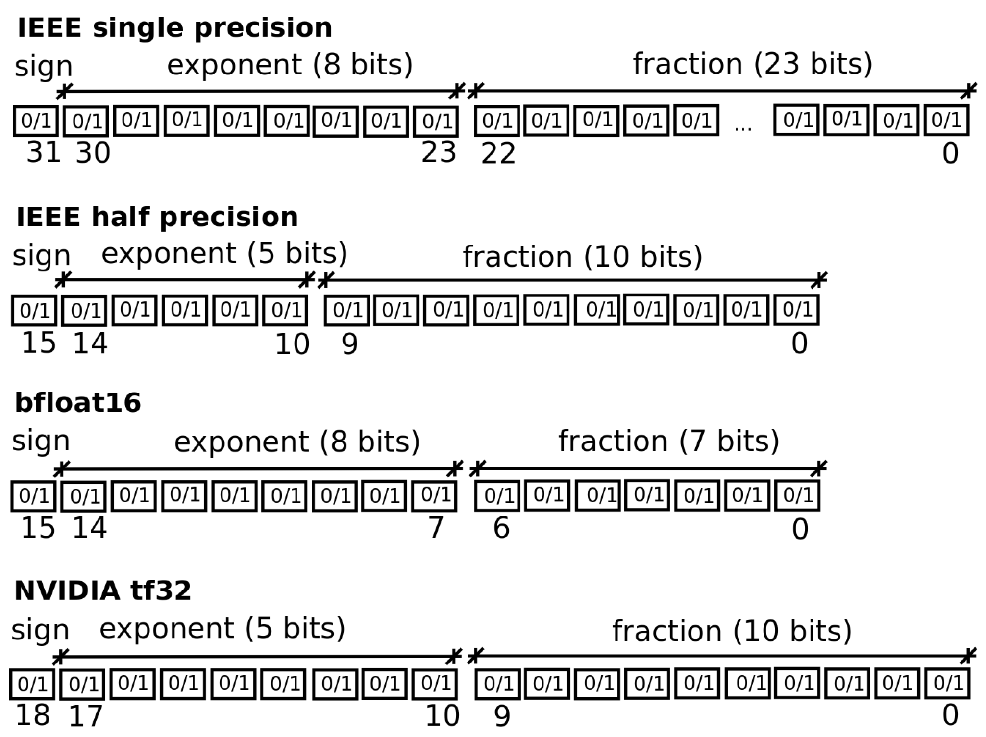
Figure 2.
Handling of the quantization error due to rounding in the case of a fixed point. This figure is constructed using the formulations in [13].
Figure 2.
Handling of the quantization error due to rounding in the case of a fixed point. This figure is constructed using the formulations in [13].
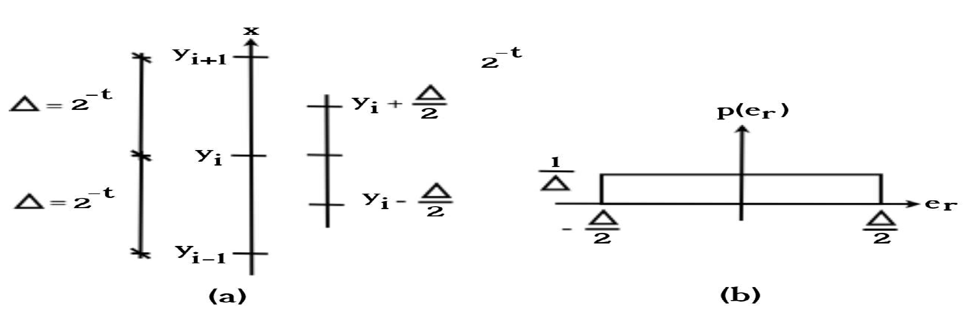
Figure 3.
Probability distribution of function . This figure is constructed using the formulations in [13].
Figure 3.
Probability distribution of function . This figure is constructed using the formulations in [13].
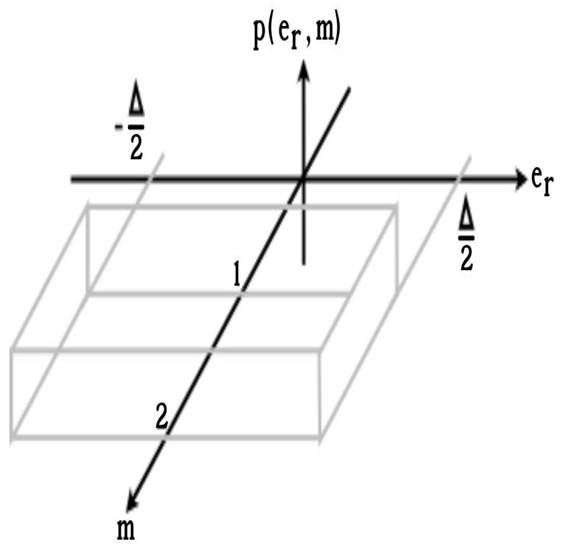
Figure 4.
Algorithms for addition and multiplication specially designed for neural networks applications [2,3,4].
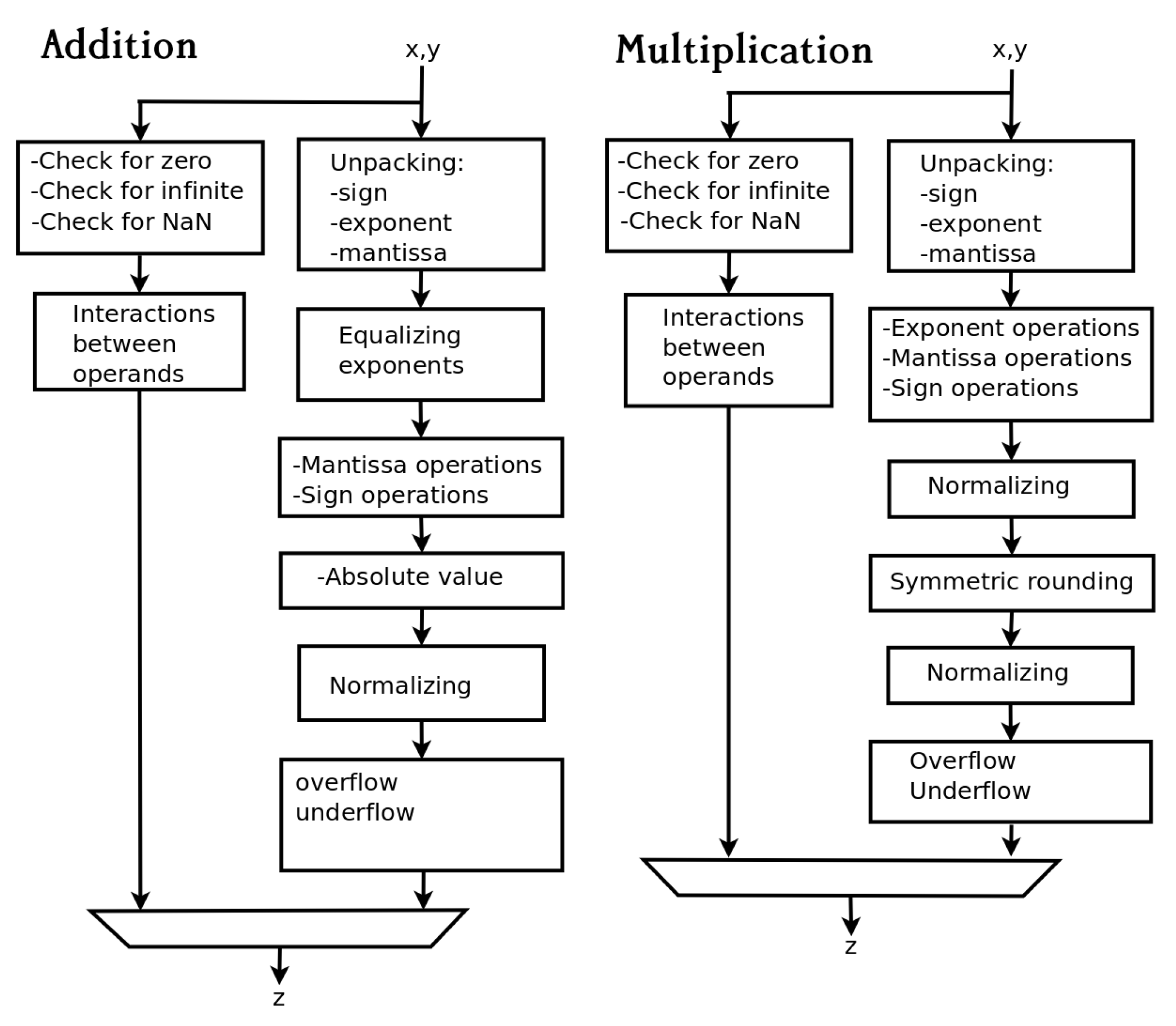
Figure 5.
Plot of calculated deviation after encoding-decoding process between fp64 and the short floating point formats fp16, fp18, fp16-20 and fp16-24. Truncation was used in these processes. The range of used values is .
Figure 5.
Plot of calculated deviation after encoding-decoding process between fp64 and the short floating point formats fp16, fp18, fp16-20 and fp16-24. Truncation was used in these processes. The range of used values is .
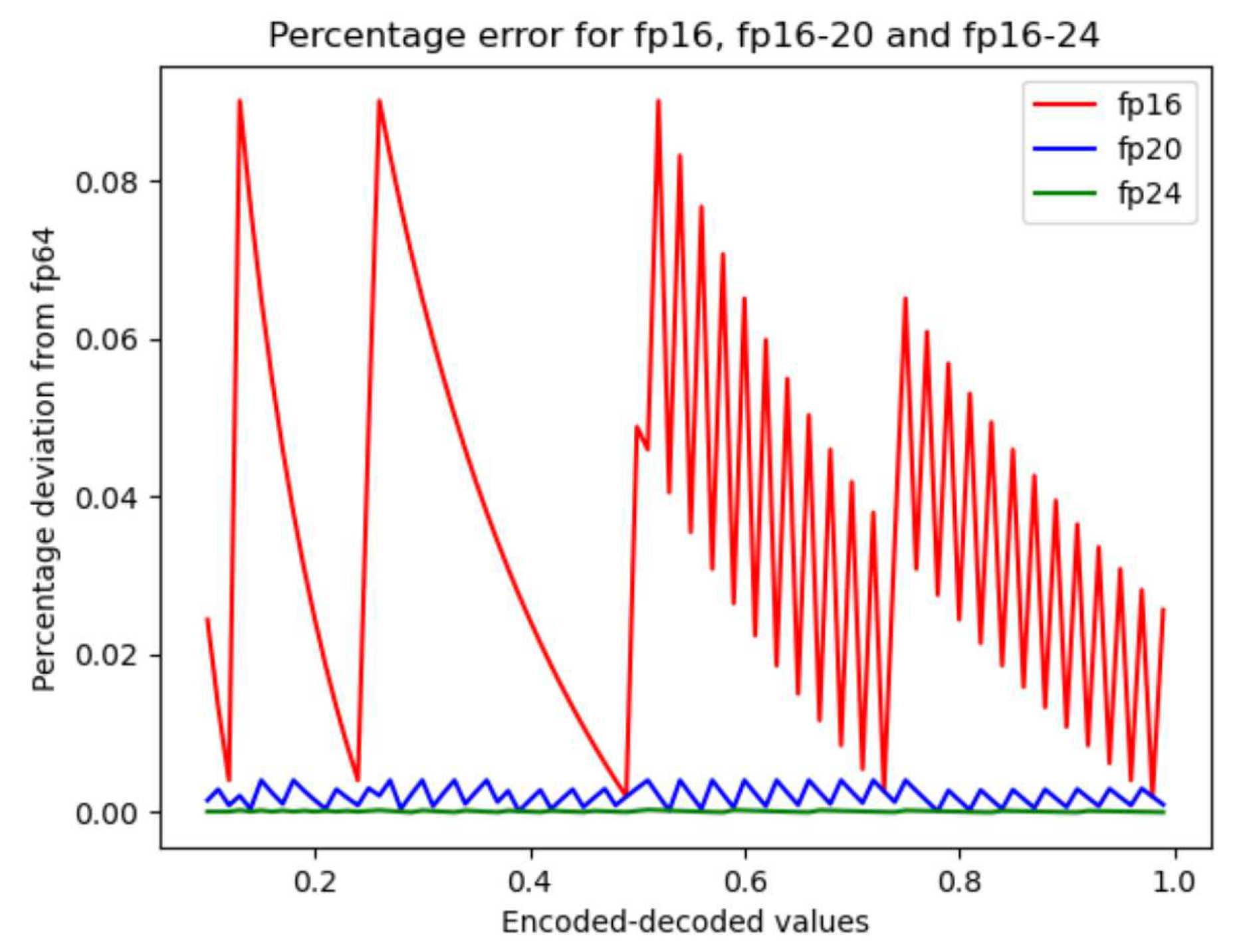
Figure 6.
Plot of calculated deviation in percentage after encoding-decoding process between fp64 and the short floating point formats fp16, fp16-20 and fp16-24. Rounding to nearest was used in these processes. The range of used values is .
Figure 6.
Plot of calculated deviation in percentage after encoding-decoding process between fp64 and the short floating point formats fp16, fp16-20 and fp16-24. Rounding to nearest was used in these processes. The range of used values is .
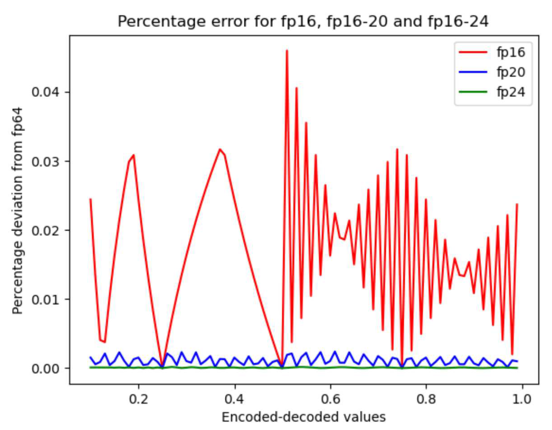

Table 1.
Features of proposed floating point data types.
| data type | sign | exponent | fraction |
|---|---|---|---|
| fp16 | 1 | 5 | 10 |
| fp16-20 | 1 | 5 | 14 |
| fp16-24 | 1 | 5 | 18 |
Table 2.
Algorithm to statistically obtain the relative error variance.
| { | |
|---|---|
| ; | |
| } | |
Table 3.
Algorithm to statistically obtain the relative error variance of Q products.
| { | |
|---|---|
| } | |
Table 4.
Fractional digits that can be encapsulated into proposed short floating point formats.
| Format | Process | Average |
|---|---|---|
| fp16 | trunc | 3.0103 |
| fp16 | round | 3.3113 |
| fp16-20 | trunc | 4.2144 |
| fp16-20 | round | 4.5154 |
| fp16-24 | trunc | 5.4185 |
| fp16-24 | round | 5.7196 |
Table 5.
Fractional digits faithful after encoding-decoding process between real number and short floating point formats.
Table 5.
Fractional digits faithful after encoding-decoding process between real number and short floating point formats.
| Format | Process | Maximun | Minimum | Average |
|---|---|---|---|---|
| fp16 | truncate | 9 | 0 | 3.013153 |
| fp16 | round | 9 | 0 | 3.288637 |
| fp16-20 | truncate | 10 | 0 | 4.199776 |
| fp16-20 | round | 10 | 0 | 4.496876 |
| fp16-24 | truncate | 12 | 0 | 5.397121 |
| fp16-24 | round | 12 | 0 | 5.721044 |
Table 6.
Variance error coding for floating point formats fp16, fp16-20 and fp16-24.
| Theoretical values | Statistical value | |
| Data type | Error variance | Error variance |
| fp16 | ||
| fp16-20 | ||
| fp16-20 |
Table 7.
Relative error variances of Q products using data type fp16, fp16-20, fp16-24.
| Length | Theoretical relative | Statistical relative | |
| Data type | Length | error variance | error variance |
| fp16 | 32 | ||
| 64 | |||
| 128 | |||
| 256 | |||
| 512 | |||
| 1024 | |||
| 2048 | |||
| fp16-20 | 32 | ||
| 64 | |||
| 128 | |||
| 256 | |||
| 512 | |||
| 1024 | |||
| 2048 | |||
| fp16-24 | 32 | ||
| 64 | |||
| 128 | |||
| 256 | |||
| 512 | |||
| 1024 | |||
| 2048 |
Table 8.
Average error calculated after each encoding-decoding process between fp64 and the short floating point formats pg16, fp18, fp16-20 and fp16-24.
Table 8.
Average error calculated after each encoding-decoding process between fp64 and the short floating point formats pg16, fp18, fp16-20 and fp16-24.
| rounding/truncation | encodig process | average error |
|---|---|---|
| Truncation | fp64 → fp16 | 0.03590 |
| fp64 → fp16-20 | 0.00212 | |
| fp64 → fp16-24 | 0.00014 | |
| Rounding | fp64 → fp16 | 0.01675 |
| fp64 → fp16-20 | 0.00106 | |
| fp64 → fp16-24 | 0.00007 |
Table 9.
Deviations calculated after performing the dot product using data types fp16, fp16-20 and fp16-24. Several dot product lengths have been tested as shown in the table.
Table 9.
Deviations calculated after performing the dot product using data types fp16, fp16-20 and fp16-24. Several dot product lengths have been tested as shown in the table.
| Data type | length | Dot product in fp64 | MAC-truncate | |
| in bits | Dec | Dec | Relative error (%) | |
| fp16 | 32 | 9.8580 | 9.7813 | 0.779 |
| 64 | 21.8639 | 21.6250 | 1.0925 | |
| 128 | 41.8754 | 40.9688 | 2.1650 | |
| 256 | 86.9919 | 83.1875 | 4.3733 | |
| 512 | 179.9733 | 164.7500 | 8.4586 | |
| 1024 | 353.0430 | 294.2500 | 16.6532 | |
| 2048 | 713.6043 | 521.5000 | 26.92029 | |
| fp16-20 | 32 | 9.8580 | 9.8438 | 0.1447 |
| 64 | 21.8639 | 21.8281 | 0.1634 | |
| 128 | 41.8754 | 41.7813 | 0.2247 | |
| 256 | 86.9919 | 86.6250 | 0.4218 | |
| 512 | 179.9733 | 178.7500 | 0.6797 | |
| 1024 | 353.0430 | 348.5000 | 1.2868 | |
| 2048 | 713.6043 | 696.5000 | 2.3969 | |
| fp16-24 | 32 | 9.8580 | 9.8438 | 0.1447 |
| 64 | 21.8639 | 21.8438 | 0.0920 | |
| 128 | 41.8754 | 41.8125 | 0.1501 | |
| 256 | 86.9919 | 86.8750 | 0.1344 | |
| 512 | 179.9733 | 179.7500 | 0.1241 | |
| 1024 | 353.0430 | 352.5000 | 0.1538 | |
| 2048 | 713.6043 | 712.0000 | 0.2248 | |
Table 10.
Continuation from Table Table 9. Deviations calculated after performing the dot product using data types fp16, fp16-20 and fp16-24. Several dot product lengths have been tested as shown in the table.
Table 10.
Continuation from Table Table 9. Deviations calculated after performing the dot product using data types fp16, fp16-20 and fp16-24. Several dot product lengths have been tested as shown in the table.
| Data type | length | Dot product in fp64 | MAC-round | |
| in bits | Dec | Dec | Relative error (%) | |
| fp16 | 32 | 9.8580 | 9.7969 | 0.620 |
| 64 | 21.8639 | 21.6407 | 1.0210 | |
| 128 | 41.8754 | 41.0000 | 2.0904 | |
| 256 | 86.9919 | 83.1875 | 4.3733 | |
| 512 | 179.9733 | 164.8750 | 8.3892 | |
| 1024 | 353.0430 | 294.2500 | 16.6532 | |
| 2048 | 713.6043 | 521.5000 | 26.92029 | |
| fp16-20 | 32 | 9.8580 | 9.8516 | 0.0654 |
| 64 | 21.8639 | 21.8438 | 0.0920 | |
| 128 | 41.8754 | 41.8125 | 0.1501 | |
| 256 | 86.9919 | 86.6875 | 0.3500 | |
| 512 | 179.9733 | 178.8750 | 0.6102 | |
| 1024 | 353.0430 | 348.7500 | 1.2160 | |
| 2048 | 713.6043 | 697.0000 | 2.3268 | |
| fp16-24 | 32 | 9.8580 | 9.8516 | 0.0654 |
| 64 | 21.8639 | 21.8594 | 0.0205 | |
| 128 | 41.8754 | 41.8438 | 0.0755 | |
| 256 | 86.9919 | 86.9375 | 0.0626 | |
| 512 | 179.9733 | 179.875 | 0.0546 | |
| 1024 | 353.0430 | 352.75 | 0.0830 | |
| 2048 | 713.6043 | 712.5 | 0.1548 | |
Table 11.
Frequencies calculated by ISE Xilinx using MAC circuits. Each MAC circuit is implemented with multiplier and adder circuits, which in turn implement circuits for fp16, fp16-20 and fp16-24. This results were calculated for XC7A100TCSG324-1 FPGA.
Table 11.
Frequencies calculated by ISE Xilinx using MAC circuits. Each MAC circuit is implemented with multiplier and adder circuits, which in turn implement circuits for fp16, fp16-20 and fp16-24. This results were calculated for XC7A100TCSG324-1 FPGA.
| circuits | Maximum Frequency calculated |
|---|---|
| fp16 | 110.106 MHz |
| fp16-20 | 101.514 MHz |
| fp16-24 | 91.189 MHz |
Table 12.
Frequencies and delays reached by several investigators in theirs experiments with floating-point implementations on FPGA. The results reached by [9,15] are reported as a comparison to understand what is the situation of the implementations reported in this article.
| Format | monoblock | Monoblock |
| delay | frequency | |
| (ns) | (MHz) | |
| sunesh fp32 [9] | 20.04 | 40 |
| fp16 | 9.08 | 110 |
| fp16-20 | 9.85 | 101 |
| fp16-24 | 10.87 | 91 |
| rao fp16 [15] | 8.82 | 113 |
Table 13.
Continuation of Table Table 12. Frequencies and delays reached by several investigators in theirs experiments with floating-point implementations on FPGA. The results reached by [9,15] are reported as a comparison to understand what is the situation of the implementations reported in this article.
| Format | Number | Maximum | Maximum frequency | Hardware |
| of | delay per | in pipeline | (FPGA) | |
| stages | stages (ns) | mode (MHz) | ||
| sunesh fp32 [9] | 4 | 7.92 | 126 | XC3S500-4FG320 |
| fp16 | 6 | 1.51 | 660 | XC7A100T-CSG324-1 |
| fp16-20 | 6 | 1.64 | 609 | XC7A100T-CSG324-1 |
| fp16-24 | 6 | 1.83 | 547 | XC7A100T-CSG324-1 |
| rao fp16 [15] | 7 | 1.26 | 793 | XC2S50E-FT256-6 |
Disclaimer/Publisher’s Note: The statements, opinions and data contained in all publications are solely those of the individual author(s) and contributor(s) and not of MDPI and/or the editor(s). MDPI and/or the editor(s) disclaim responsibility for any injury to people or property resulting from any ideas, methods, instructions or products referred to in the content. |
© 2023 by the authors. Licensee MDPI, Basel, Switzerland. This article is an open access article distributed under the terms and conditions of the Creative Commons Attribution (CC BY) license (http://creativecommons.org/licenses/by/4.0/).
Copyright: This open access article is published under a Creative Commons CC BY 4.0 license, which permit the free download, distribution, and reuse, provided that the author and preprint are cited in any reuse.


