
Submitted:
03 July 2023
Posted:
04 July 2023
You are already at the latest version
Abstract
The quadratic polynomial differential systems in the plane are the easiest nonlinear differential systems. They have been studied intensively due to their nonlinearity and to their big number of applications. These systems can be classified in ten classes. Here we provide all the topologically different phase portraits in the Poincaré disc of two of these classes.
Keywords:
quadratic vector fields
; quadratic systems
; phase portraits
MSC: Primary 34C05; 34A34; 34C14
1. Introduction and Statement of the Main Results
A quadratic polynomial differential system or simply a quadratic system is a differential system of the form
where P and Q are real polynomials in the variables x and y and the maximum degree of the polynomials P and Q is two.
At the beginning of the XX century started to be studied the quadratic systems. In [5] Coppel said that Büchel [3] in 1904 published the first work on quadratic systems. Two short surveys on quadratic systems were published by Coppel [5] In 1966, and by Chicone and Tian [4] in 1982.
During these last decades quadratic systems were studied intensively and many good results on them were obtained, see the books [2,12,13] and the references therein. Although quadratic systems have been studied in more than one thousand papers, we are far for a complete understanding of these systems.
In [8] it is proved that any quadratic system is affine-equivalent, scaling the time variable if necessary, to a quadratic system of the form
where is one of the following ten:
Roughly speaking the Poincaré disc is the disc centered at the origin of and radius one, where the interior of this disc is identified with the whole plane and its boudary the circle is identified with the infinity of the plane , because in the plane we can go to infinity in as many directions as points has the circle . For more details on the Poincaré compactification see subsection 2.2.
The aim of this paper is to classify the different phase portraits in the Poincaré disc of the classes of quadratic systems VII and VIII, i.e. of the systems
and
respectively.
Our main result is the following one.
Theorem 1.
The following two statements hold.
- (a)
- The family of quadratic systemsVII has 27 topologicvally different phase portraits in the Poincaré disc.
- (b)
- The family of quadratic systemsVIII has 25 topologicvally different phase portraits in the Poincaré disc.
The paper is organized as follows. In Section 2 we recall the basic results that we need about singular points and the Poincaré compactification. In Section 3 and Section 4 first we study the local phase portraits of the finite singular points, after we study the local phase portraits of the infinite singular points, and finally we analyze the phase portraits of the quadratic systems (2) and (3) in the Poincaré disc, respectively.
2. Preliminary Definitions
The study of the phase portraits of the quadratic systems always begin with the study of the local phase portraits of their singularities, finite and infinite, followed by the study of their separatrix connections and of their limit cycles.
In this section we introduce the basic definitions and notations that we will need for the analysis of the local phase portraits of the finite and infinite singular points.
2.1. Singular Points
A point is said to be singular point of a polynomial differential system (1) if . If the real part of the eigenvalues of the linear part of system (1) at the singular point q are not zero, then q is a hyperbolic singular point and its possible phase portraits are well known, see for instance Theorem 2.15 of [7]. If only one of the eigenvalues of the linear part of system (1) at the singular point q is zero, then q is called a semi-hyperbolic singular point, whose possible local phase portraits are also well known, see among others Theorem 2.19 of [7]. When both eigenvalues of the linear part of system (1) at the singular point q are zero but the linear part is not identically null, then q is a nilpotent singular point and again its local phase portraits are known, see for instant Theorem 3.5 of [7]. Finally when the linear part of system (1) at the singular point q is identically zero, then we say that q is degenerate or q is linearly zero. The local phase portraits of a such singular point can be studied using the change of variables called blow-ups, see for instance [1].
2.2. Poincaré Compactification
Let be the vector field defined by the polynomial differential system (1). Roughly speaking the Poincaré compactification consists in creating a vector field in a 2–dimensional sphere such that its phase portrait in the open northern and southern hemispheres is a copy of the phase portrait of the vector field X, and the equator of the sphere plays the role of the infinity of the phase portrait of X, see for details [9], or Chapter 5 of [7]. In this way we can study the orbits of the vector field X which goes to or comes from the infinity.
Let be the Poincaré sphere. We denote by the tangent plane to at a point . We consider the vector field X defined on the plane . Then the central projection defines two copies of X in , one in the northern hemisphere and the other in the southern hemisphere. Obviously the equator , represents the infinity of . The projection of the closed northern hemisphere of on under is called the Poincaré disc, and it is denoted by . As is a differentiable manifold, we define six local charts , and for with the corresponding diffeomorphisms and for which are the inverses of the central projections from the tangent planes at the points , , , , and , respectively.
We denote by the value of or for any so a few simple calculations lead for the following formulae in the corresponding local charts (see Chapter 5 of [7]):
where d is the degree of the polynomial differential system (1). The formulae for are similar to the one for with a multiplicative factor . In these coordinates for , the points of the infinity satisfy .
3. Proof of Statement of Theorem 1
3.1. Finite Singular Points
We are going to determine the local phase portrait at the finite singular points of the quadratic system (2).
Assume first . If then the finite singular points of system (2) are
The eigenvalues of the Jacobian matrix of system (2) at are 0 and . So from Theorem 2.19 of [7] we have that and are semi-hyperbolic saddle-nodes.
If there are no finite singular points.
If then and . The Jacobian matrix of the differential system at p is
If then this singular point is nilpotent, and from Theorem 3.5 of [7], this singular point is a saddle-node.
If the linear part of the differential system at the equilibrium point p is identically zero, and the differential system becomes a homogeneous quadratic differential system. Using the results of Date in [6] who classify the phase portraits of all the homogeneous quadratic systems we obtain that the phase portraits of system (3) when are given in Figure 1 according the sign of n, If then the phase portraits of system (3) are given in Figure 3 according with the sign of n. Finally if the phase portraits of system (3) are given in Figure 2 according with the sign of n.
We assume now In this case if there exists a unique singular point namely , and the eigenvalues of the Jacobian matrix at q are 0 and b. If then q is a semi-hyperbolic saddle-node by Theorem 2.19 of [7]. If and the differential system has no finite equilibria. If then the system has a straight line filled with equilibria and we do not consider this kind of differential systems because this case can be reduced to a linear differential system doing a rescaling in the independent variable.
In summary we have proved the following proposition.
Proposition 1.
Assume that .
- (a)
- If the differential system (2) has two finite equilibria that are semi-hyperbolic saddle-nodes.
- (b)
- If the differential system (2) has no finite equilibria.
- (c)
-
.
- (c.1)
- If the differential system (2) has one finite equilibrium point p that is a nilpotent saddle-node.
- (c.2)
- .
- (c.2.1)
- (c.2.2)
- (c.2.3)
Assume that .
We assume now In this case if there exists a unique singular point namely , and the eigenvalues of the Jacobian matrix at q are 0 and b. If then q is a semi-hyperbolic saddle-node by Theorem 2.19 of [7]. If and the differential system has no finite equilibria. If then the system has a straight line filled with equilibria and we do not consider this kind of differential systems because this case can be reduced to a linear differential system doing a rescaling in the independent variable.
3.2. The Infinite Singular Points in the Chart
System (refe2x) in the local chart writes
Assume the infinite singular points are
The eigenvalues of the Jacobian matrix at are . If they are real, then and is a hyperbolic saddle and is a hyperbolic stable node. If then . In this case the Jacobian matrix writes
and the eigenvalues are -1 and 0, wich means that the unique singular point in the chart it is semi-hyperbolic and from Theorem 2.19 of [7] is a semi-hyperbolic saddle-node.
3.3. The Infinite Singular Point at the Origin of the Chart
Studying the infinite singular points in the local chart we also have studied the infinite singular points in the local chart . So only remains to see if the origins of the local charts and are infinite singular points or not.
System (2) in the local chart writes
so the origin of always is an infinite singular point. The eigenvalues of the Jacobian matrix of system (8) at the origin are with multiplicity two. Therefore the origin is a hyperbolic stable node if , and unstable node if .
If then the Jacobian matrix of the system at the origin of the local chart is the zero matrix and we need to make blow-ups in order to study its local phase portrait. Before doing a vertical blow-up we need to be sure that is not a characteristic direction. If is a characteristic direction then u is a factor of the polynomial , where and are the terms of degree two of and . In our case . So is a characteristic direction and consequently before doing a vertical blow-up, we must do a twist in order that do not be a characteristic direction. This is done with the change of variables where , . Doing this change of variables the differential system (8) writes
Since is not a characteristic direction we can do a vertical blow-up. This vertical blow-up is given by the change of variables where Then system (6) becomes
Now doing a rescaling of the time with the factor we obtain the system
The singular points of system (11) on are and which is double. The eigenvalues of the Jacobian matrix at are and . So the point is a hyperbolic stable node if , a hyperbolic saddle if , and for a sami-hyperbolic saddle-node according to Theorem 2.19 of [7]. The eigenvalues of the Jacobian matrix at are 0 and . So the local phase portrait of the origin of the local chart is shown in Figure 4(a) when , and .
Starting from Figure 4(a) we obtain the local phase portrait at the axis of system (10): see Figure 4(b) and going back through the vertical blow, taking into account the value of we obtain the local phase portrait at the origin of system (5) in Figure 4(c). Finally undoing the twist we get the local phase portrait at the origin of the local chart which is shown in Figure 4(d) and Figure 5(a).
Working in a similar way to the preceding case, doing the convenient blow ups and using Theorems 2.15 and 2.19 of [7] we obtain all the local phase portraits at the origin of the local chart in Figure 5. All those local phase portraits are then the following
, and in Figure 5(a);
, and in Figure 5(b);
, and in Figure 5(c);
, and in Figure 5(d);
, , and in Figure 5(e);
, , and then is a stright line of singular points;
, , and in Figure 5(f);
, , and then is a stright line of singular points;
, , and in Figure 5(g);
, , and in Figure 5(h);
, , and in Figure 5(i);
, , and in Figure 5(j);
, , and in Figure 5(k);
, , and in Figure 5(l);
, and then is a stright line of singular points.
3.4. The Global Phase Portaits
The preceding results for the finite and infinite singular points, allow to obtain the global phase portraits quite easily, taking into account that the straight line is invariant.
First we consider the case satisfying the following conditions: , and . We have seen that if then there is a stable hyperbolic node at the origin of the chart . Since there exist two real finite singular points and that are semi-hyperbolic saddle-nodes. Finitely since imply the existence of two infinite singular points in the chart ( is a hyperbolic saddle and a hyperbolic node). The local phase portraits at all these singular points are shown in Figure 6. The tools for studying the phase portraits in this case are employed for all possible configurations which appears in Figure 7.
, and in Figure 7(1) to Figure 7(4), but the phase portrait in Figure 7(2) appears by continuity between the phase portraits in Figure 7(1) to Figure 7(3);
, and from Figure 7(5);
, , and in Figure 7(9);
, , and in Figure 7(10);
, , in Figure 7(11);
The phase portraits with are symmetric with respect to the origin of coordinates of the preceding eight cases.
Now we study the phase portraits when .
, and in Figure 7(21);
, and in Figure 7(22);
, and in Figure 7(23);
The cases with are the symmetric with respect to the origin of coordinates of the preceding three cases.
, , and in Figure 7(24);
The cases with are the symmetric with respect to the origin of coordinates of all the preceding case.
, , and in Figure 7(25);
The cases with are the symmetric with respect to the origin of coordinates of all the preceding case.
, , and in Figure 7(26);
, , and in Figure 7(27).
Of course from the Table 1 the phase portraits with different number of separatrices and canonical regions are topologically distinct. Now we shall see that the phase portraits with the same number of separatrices and canonical regions of the Table 1 also are topologically different.

Table 1.
Here p.p. denotes phase portrait in the Poincaré disc, s denotes the number of separaratrices of the phase portrait, and r denotes the number of canonical regions of the phase portrait.
Table 1.
Here p.p. denotes phase portrait in the Poincaré disc, s denotes the number of separaratrices of the phase portrait, and r denotes the number of canonical regions of the phase portrait.
| s | 4 | 5 | 6 | 8 | 9 | 9 | 10 | 11 | 12 |
| r | 1 | 2 | 2 | 3 | 4 | 2 | 3 | 4 | 3 |
| p.p. | 10 | 26,27 | 14 | 15 | 23 | 25 | 11,24 | 5 | 18,22 |
| s | 13 | 14 | 14 | 16 | 17 | 18 | 19 | 20 | 21 |
| r | 4 | 3 | 5 | 5 | 6 | 5 | 6 | 5 | 6 |
| p.p. | 16,19,20 | 9 | 17,21 | 8 | 6,7 | 13 | 12 | 2 | 1,3,4 |
The phase portraits 26 and 27 of Figure 7 are topologically different because the phase portrait 27 has two elliptic sectors and the phase portrait 26 has no elliptic sectors.
The phase portraits 11 and 24 of Figure 7 are topologically different because the phase portrait 24 has two elliptic sectors and the phase portrait 11 has no elliptic sectors.
The phase portraits 18 and 22 of Figure 7 are topologically different because the phase portrait 18 have orbits starting at the origin of the local chart and ending at the origin of the local chart , and this kind of orbits do not exist in the phase portrait 22.
The phase portraits 16, 19 and 20 of Figure 7 are topologically different. First the phase portrait 16 have orbits starting at the origin of the local chart and ending at the origin of the local chart , and this kind of orbits do not exist in the phase portrait 19 and 20. The phase portrait 19 has a separatrix starting at the origin of the local chart and ending at an infinite equilibrium point in the local chart , and such a kind of separatrix does not exist in the phase portrait 20.
The phase portraits 17 and 21 of Figure 7 are topologically different because the phase portrait 21 has two elliptic sectors and the phase portrait 17 has no elliptic sectors.
The phase portraits 1, 3 and 4 of Figure 7 are topologically different because the unstable separatrix of the lower equilibrium point on the straight line contained in has different ending infinite equilibrium point in the these three phase portraits.
4. Proof of Statement Theorem 1
4.1. Finite Singular Points
We are going to analyze the singular points of the quadratic system (3).
Assume first . The finite singular points of system (3) are
If , the eigenvalues of the Jacobian matrix of system (3) at are 1 and . So from Theorem 2.15 of [7] we have is a hyperbolic unstable node and is a hyperbolic saddle. If then . The eigenvalues of the Jacobian matrix of system (3) at p are therefore by Theorem 2.19 of [7] we obtain that p is a semi-hyperbolic saddle-node. Of course, if there are no finite singular points.
We assume now In this case if there exists a unique singular point namely , and the eigenvalues of the Jacobian matrix at p are 1 and b. If then p is a hyperbolic unstable node. If then p is a hyperbolic saddle. If there are no finite singular points.
4.2. the Infinite Singular Points in the Chart
System (3) in the local chart writes
Assume the infinite singular points are
if . If then . The eigenvalues of the Jacobian matrix at are 0 and . By Theorem 2.19 of [7] we get are semi-hyperbolic saddle-nodes. The Jacobian matrix at P is
If then P is a nilpotent singular point, and by Theorem 3.5 of [7] is a saddle-node. If , then P is degenerate. If we translate the singular point P to the origin it becomes a homogeneous quadratic system and their phase portraits have been classified by Date in [6]. It follows that if we obtain that the local phase portrait at P on the Poincaré sphere is formed by two hyperbolic sectors separated by two parabolic ones, the infinity separates the two hyperbolic sectors which have one separatrix at infinity. If , then the local phase portrait at P is a node, unstable if , and stable if .
4.3. the Infinite Singular Point at the Origin of the Chart
Studying the infinite singular points in the local chart we also have studied the infinite singular points in the local chart . So only remains to see if the origins of the local charts and are infinite singular points or not.
System (3) in the local chart writes
so the origin of always is an infinite singular point. The eigenvalues of the Jacobian matrix of the system at the origin are with multiplicity two. Therefore the origin is a hyperbolic node, stable if , and unstable if .
If then the Jacobian matrix of the system at the origin is the zero matrix and we need to make blow-ups in order to study the local phase portrait at the origin of . Before doing a vertical blow-up we need to be sure that is not a characteristic direction. If is a characteristic direction then u is a factor of the polynomial , where and are the terms of lowest degree of and . In our case . So is characteristic direction and consequently before doing a vertical blow-up, we must do a twist in order that do not be a characteristic direction. This is done with the change of variables where , . Doing this change of variables the differential system (8) writes
The characteristic directions of this system are given by the polynomial , so is not a characteristic direction and we can do a vertical blow-up. This vertical blow-up is given by the change of variables where Then system (9) becomes
Now doing a rescaling of the time with the factor we obtain the system
The singular points of system (11) on are which is double and . The eigenvalues of the Jacobian matrix at are 0 and . So the is a semi-hyperbolic singular point, applying to it Theorem 2.19 of [7] it is a saddle-node. The eigenvalues of the Jacobian matrix at are 1 and . So this singular point is hyperbolic, a saddle if , an unstable node if , see Figure 8(a) when , and .
From Figure 8(a) we obtain that the local phase portrait at the axis of system (10) is given in Figure 8(b). Now going back through the vertical blow up and taking into account the value of we obtain the local phase portrait at the origin of system (8) in Figure 8(c). Finally unding the twist we get the local phase portrait at the origin of the local chart which is shown in Figure 8(d) and Figure 9(a).
Working in a similar way to the case , and , i.e. doing the convenient blow ups and using Theorems 2.15 and 2.19 of [7] we obtain all the local phase portraits at the origin of the local chart in Figure 9 for the following cases:
, and in Figure 9(b);
, , , and in Figure 9(c);
, and , in Figure 9(d);
, and in Figure 9(e);
, and in Figure 9(f);
, , and in Figure 9(g);
, , and in Figure 9(h);
, , and in Figure 9(i);
, , and in Figure 9(j);
, , and in Figure 9(k);
, , , and in Figure 9(l);
, , , and in Figure 9(m);
, , , and in Figure 9(n);
, , and in Figure 9(o);
, , and in Figure 9(p);
, , , and in Figure 9(q);
, , and in Figure 9(r).
4.4. The Global Phase Portaits
The preceding results for the finite and infinite singular points, allow to obtain the global phase portraits quite easily, taking into account that the straight line is invariant.
First we consider the case satisfying the following conditions: , and . We have seen that denotes a stable hyperbolic node at the origin of the chart , indicates the existence of two real finite singular points ( a hyperbolic unstable node and a hyperbolic saddle), and imply two infinite singular points in the chart ( and which are nilpotent saddle-nodes). The local phase portraits at all these singular points are shown in Figure 10.
With the help of Mathematica we have proved that in order that the conditions , and hold, the parameters of the differential system (3) must satisfy one of the conditions:
- (i)
- , , and ;
- (ii)
- , , , and ;
- (iii)
- , , , and ;
- (iv)
- , , and ;
- (v)
- , , , and ;
- (vi)
- , , , and ;
- (vii)
- , , and ;
- (viii)
- , , , and ;
- (ix)
- , , , and ;
- (x)
- , , and ;
- (xi)
- , , , and ;
- (xii)
- , , , and ;
- (xiii)
- , , and ;
- (xiv)
- , , , and ;
- (xv)
- , , , and .
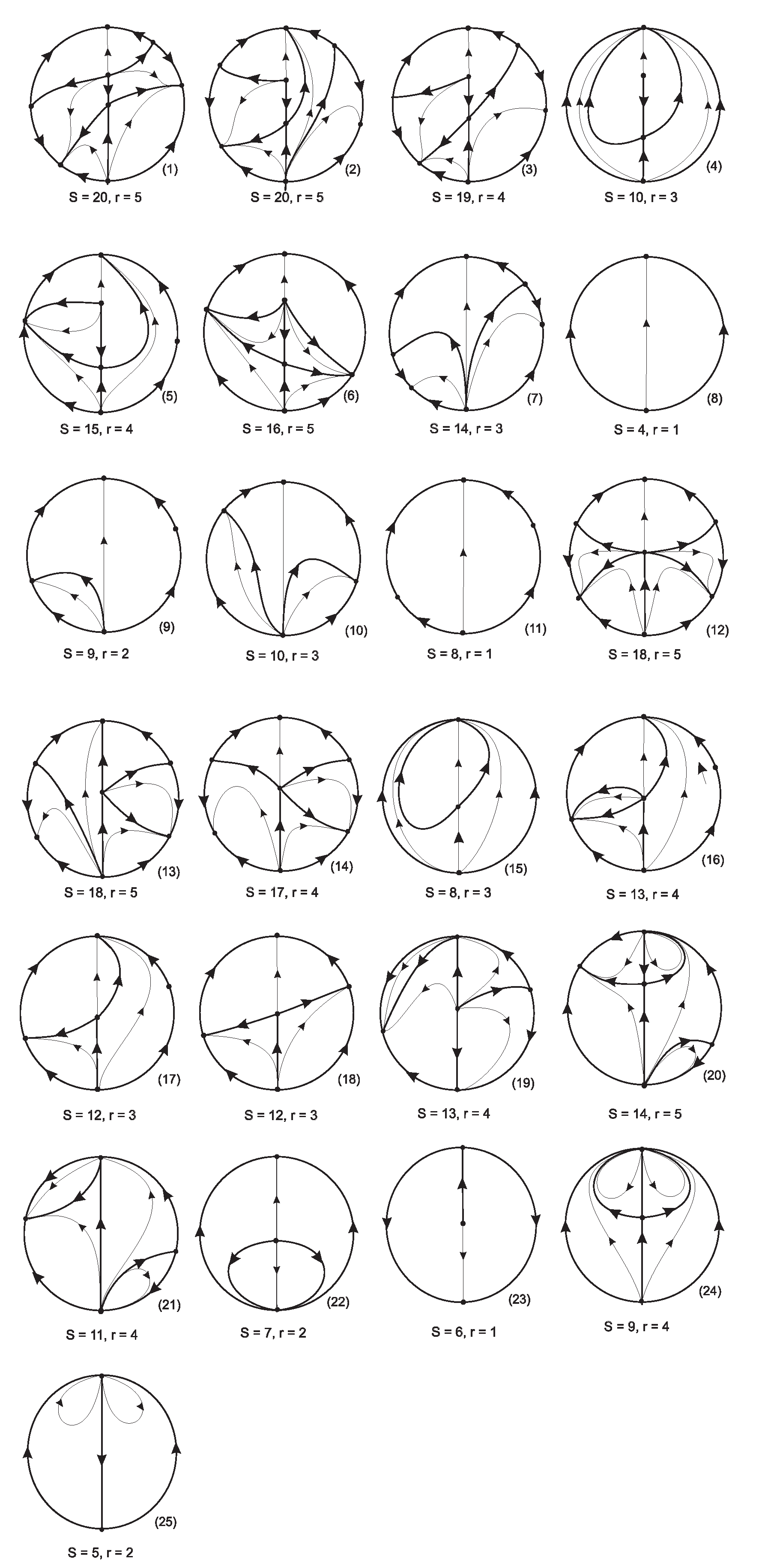
We have proved that in the cases (i), (ii), (iv), (vii) and from (ix) to (xv) we get the phase portrait (1) of Figure 11; in the cases (iii), (vi) and (viii) we obtain the phase portrait (2) of Figure 11; and finally in the case (v) we get the phase portrait symetric to the phase portrait (2) with respect to the straigt line . For instance: the phase portrait (1) of Figure 11 is obtained when the parameters of system (3) are , , , and ; the phase portrait (2) of Figure 11 is obtained when the parameters are , , , and .The phase portrait (3) of Figure 11 exists by continuity going from the phase portrait (1) to the phase portrait (2).
We recall that the separatrices of a polynomial differential system in the Poincaré disc are all the orbits at infinity, the finite singularities and the two orbits at the boundary of an hyperbolic sector. Also the limit cycles are separatrices but the quadratic system VIII has no limit cycles. If in a phase portrait of the Poincaré disc we remove all the separatrices the open components which remain are called the the canonical regions of the phase portrait. For more details on the separatrices and canonical regions see [10,11].
The tools for studying the phase portraits of system (3) for the case , and are used in the following cases, leading to the next results:
, , and in Figure 11(4);
, , and in Figure 11(5);
, , and in this case the phase portrait is symmetric with respect to the straight line of the phase portrait of the previous case;
, , and in Figure 11(6);
, , and in Figure 11(7);
, , and in Figure 11(8);
, , and in Figure 11(9);
, , and this case is a symetric phase portrait with respect to the straight line of the previous phase phase portrait;
, , and in Figure 11(15);
, , and in Figure 11(18);
The cases with are the symetric with respect to the straight line to all the preceding cases;
, in Figure 11(19);
, in Figure 11(20);
, and in Figure 11(21);
, and this case has a symmetric phase portrait with respect to to the previous case;
The phase portraits of the cases and are symmetric with respect to the straight line of the phase portraits of the cases and
, and in Figure 11(22);
, and this case has a symetric phase portrait with respect to the axis;
, and in Figure 11(23);
, and in Figure 11(24);
, and the phase portrait of this case is symetric with respect to the straight line of the previous phase portrait;
, , and in the Figure 11(25);
, , and the phase portrait of this case is symetric with respect to the straight line of the previous phase portrait;
, , and this case has the same phase portrait of Figure 11(8);
, , and this case has the symetric phase portrait with respect to the straight line to the phase portrait of Figure 11(8).
Of course from the Table 2 the phase portraits with different number of separatrices and canonical regions are topologically distinct. Now we shall see that the phase portraits with the same number of separatrices and canonical regions of the Table 2 also are topologically different.
The phase portraits 4 and 10 of Figure 12 are topologically different because the phase portrait 4 has two finite singular points and the phase portrait 10 has no finite singular points.
Table 2.
Here p.p. denotes phase portrait in the Poincaré disc, s denotes the number of separaratrices of the phase portrait, and r denotes the number of canonical regions of the phase portrait.
Table 2.
Here p.p. denotes phase portrait in the Poincaré disc, s denotes the number of separaratrices of the phase portrait, and r denotes the number of canonical regions of the phase portrait.
| s | 4 | 5 | 6 | 7 | 8 | 8 | 9 | 9 | 10 | 11 |
|---|---|---|---|---|---|---|---|---|---|---|
| r | 1 | 2 | 1 | 2 | 1 | 3 | 2 | 4 | 3 | 4 |
| p.p. | 8 | 25 | 23 | 22 | 11 | 15 | 9 | 24 | 4,10 | 21 |
| s | 12 | 13 | 14 | 14 | 15 | 16 | 17 | 18 | 19 | 20 |
| r | 3 | 4 | 3 | 5 | 4 | 5 | 4 | 5 | 4 | 5 |
| p.p. | 17,18 | 16,19 | 7 | 20 | 5 | 6 | 14 | 12,13 | 3 | 1,2 |
The phase portraits 17 and 18 (respectively 16 and 19) of Figure 12 are topologically different because the phase portrait 17 (respectively 16) has two orbits going to the origin of the chart , and such orbits do not exist in the phase portrait 18 (respectively 19).
The phase portrait 14 of Figure 12 has three pairs of infinite singular points while the phase portrats 16 and 19 only have only two pairs of infinite singumlar, so the phase portrait 14 is different from the phase portraits 16 and 19.
We note that the phase portrait 13 of Figure 12 has three pairs of infinite singular points, while the phase portrait 20 has only two pairs, so these two phases portraits are topologically disctinct.
Acknowledgments
The second author is partially supported by the Agencia Estatal de Investigación grant PID2019-104658GB-I00, the H2020 European Research Council grant MSCA-RISE-2017-777911, the Generalitat de Catalunya grant 2021 SGR 00113, and by the Acadèmia de Ciències i Arts de Barcelona.
References
- M.J. Álvarez, A. Ferragud and X. Jarque, A survey on the blow up technique, Int. J. Bifur. Chaos 2011, 21, 3103–3118. [CrossRef]
- J.C. Artés, J. Llibre, D. Schlomiuk and N. Vulpe, Geometric Configurations of Singularities of Planar Polynomial Differential Systems. A Global Classification in the Quadratic Case, Birkhäuser, 2021. [CrossRef]
- W. Büchel, Zur topologie der durch eine gewöhnliche differentialgleichung erster ordnung und ersten grades definierten kurvenschar, Mitteil. der Math. Gesellsch. in Hamburg 4 (1904), 33–68.
- C. Chicone and J. Tian, On general properties of quadratic systems, The American Mathematical Monthly, Vol. 89, No. 3 (Mar., 1982), pp. 167–178. [CrossRef]
- W.A. Coppel, A Survey of Quadratic Systems, J. Differential Equations 2 (1966), 293–304.
- T. Date, Classification and analysis of two-dimensional real homogeneous quadratic differential equation systems, J. Differential Equations 21, (1979), 311–334. [CrossRef]
- F. Dumortier, J. F. Dumortier, J. Llibre and J.C. Artés, Qualitative theory of planar differential systems, Universitext, Springer–Verlag, 2006. [CrossRef]
- A. Gasull, Sheng Li-Ren and J. Llibre, Chordal quadratic systems, Rocky Mountain J. of Math. 16, (1986), 751–782.
- E. A. González, Generic properties of polynomial vector fields at infinity. Trans. Amer. Math. Soc. 1969, 143, 201–222. Trans. Amer. Math. Soc. [CrossRef]
- L. Markus, Quadratic differential equations and non-associative algebras, Annals of Mathematics Studies, Vol 45, Princeton University Press, 1960, pp 185–213. [CrossRef]
- D. Neumann, Classification of continuous flows on 2-manifolds. Proc. Amer. Math. Soc. 1975, 48, 73–81. [CrossRef]
- J. Reyn, Phase Portraits of Planar Quadratic Systems, Mathematics and Its Applications vol. 583, Springer, 2007.
- Y. Ye, Theory of imit cycles, Transl. Math. Monogr., vol. 66, Amer. Math. Soc., Providence, RI, 1986.
Figure 1.
.
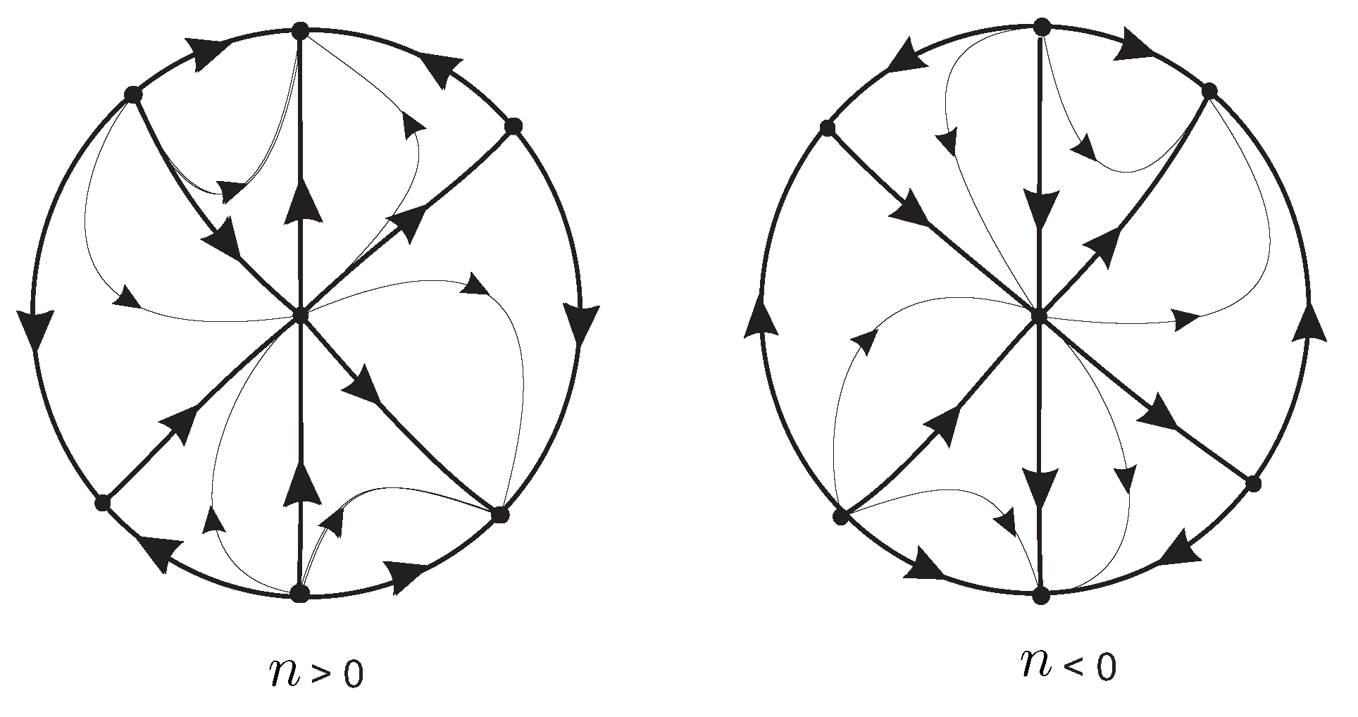
Figure 2.
.
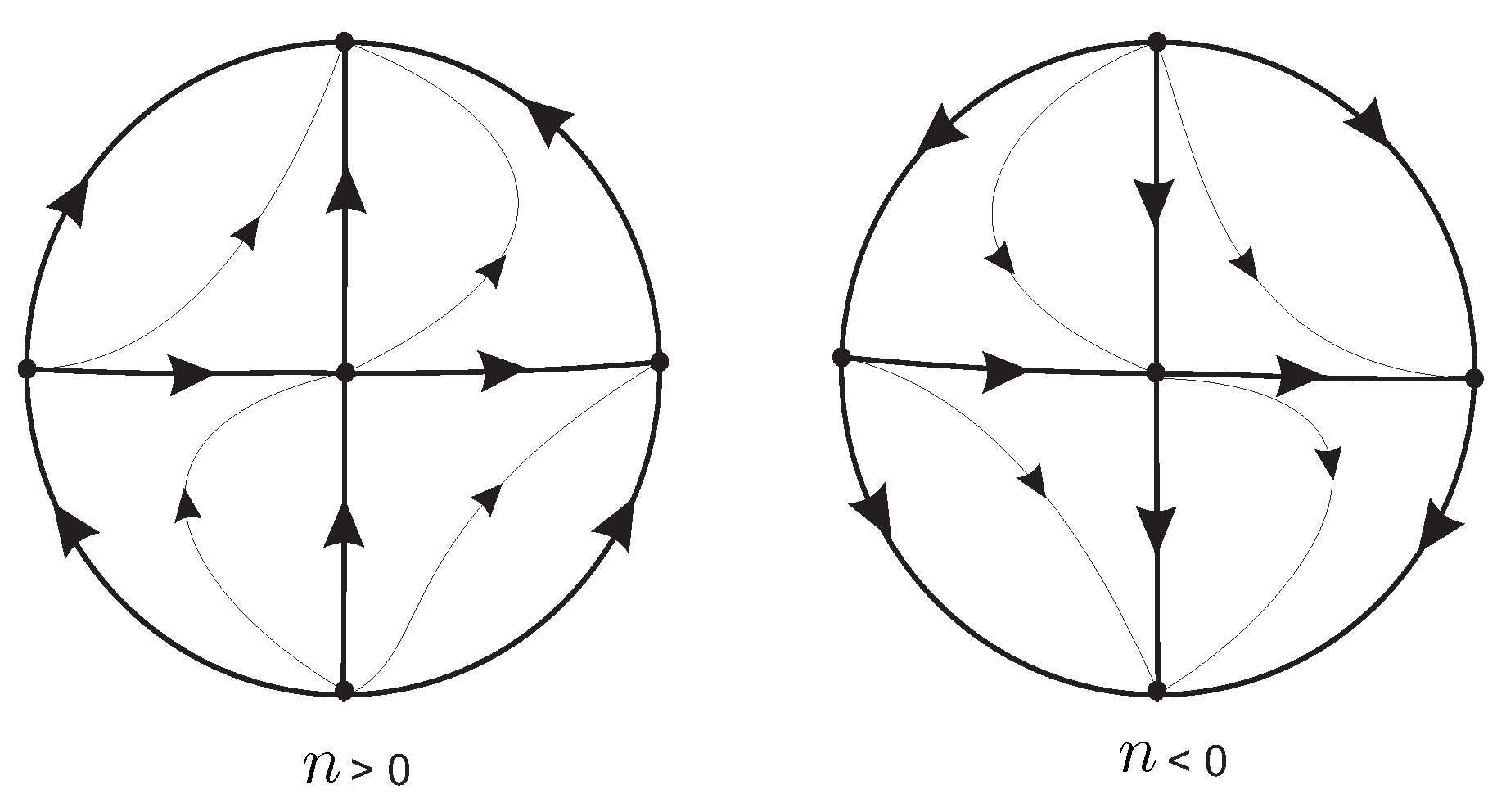
Figure 3.
.
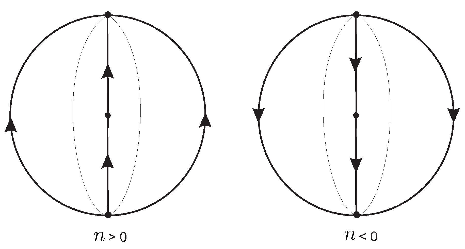
Figure 4.
The sequences of blow-ups for obtaining the local phase portrait at the origin of the local chart when , and .
Figure 4.
The sequences of blow-ups for obtaining the local phase portrait at the origin of the local chart when , and .
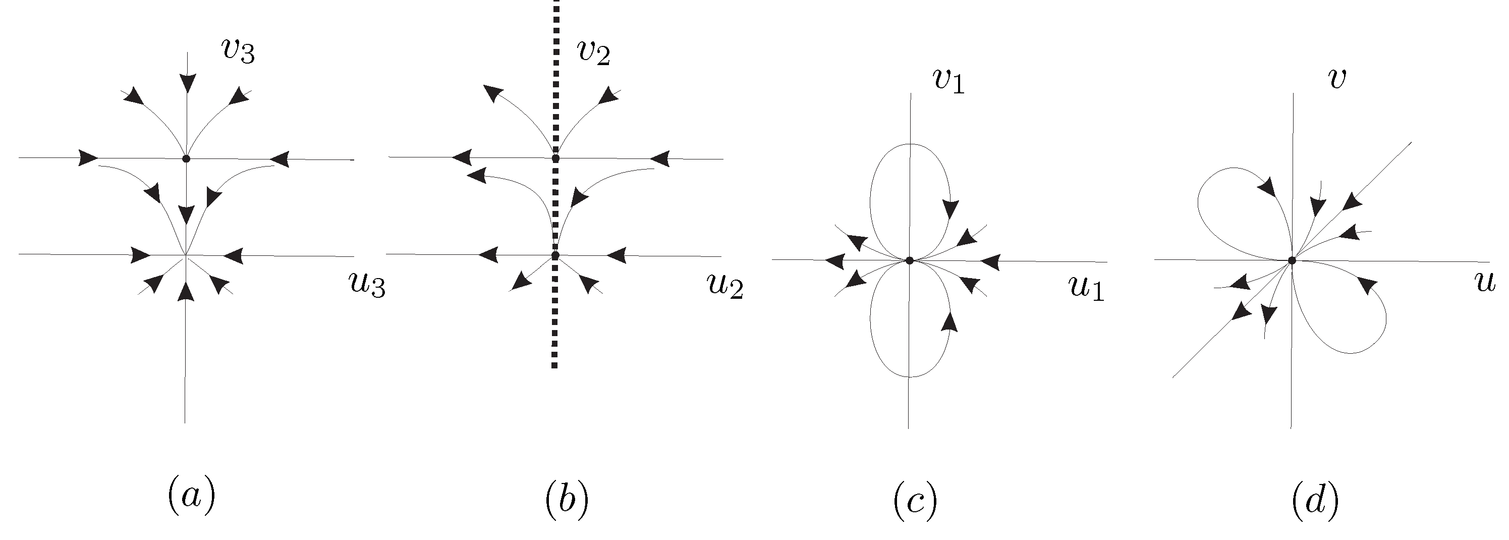
Figure 5.
The distinct topological local phase portraits at the origin of the local chart .
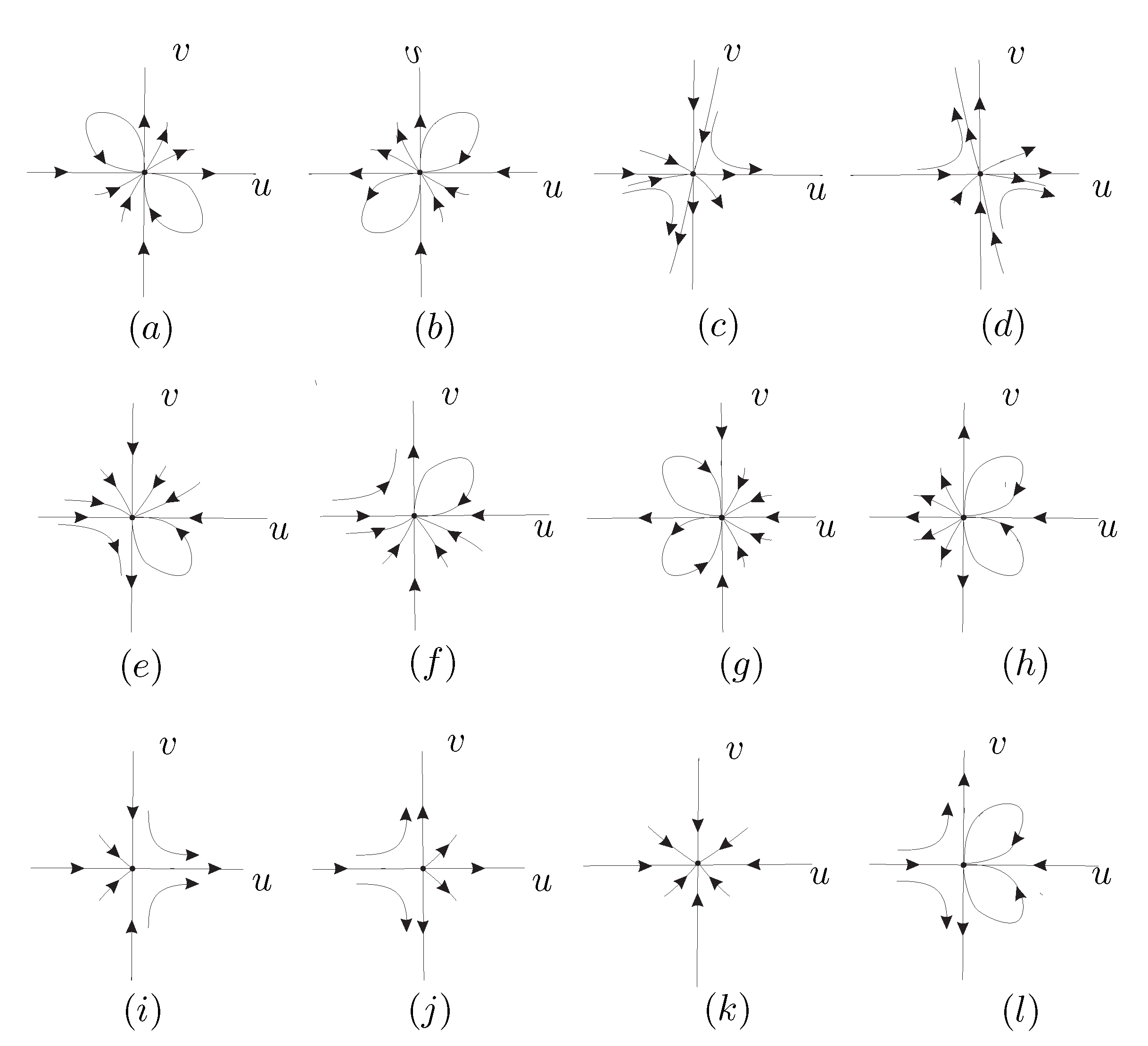
Figure 6.
The local phase portraits at the finite and infinite singular points for the case , and .
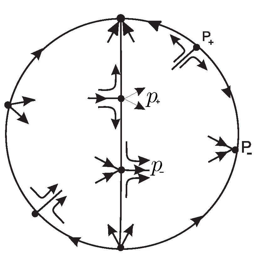
Figure 7.
All the distinct topological phase portraits of the quadratic systems VII. Here s (respectively r) denotes the number of separatrices of a phase portrait in the Poincaré disc (respectively canonical regions).
Figure 7.
All the distinct topological phase portraits of the quadratic systems VII. Here s (respectively r) denotes the number of separatrices of a phase portrait in the Poincaré disc (respectively canonical regions).
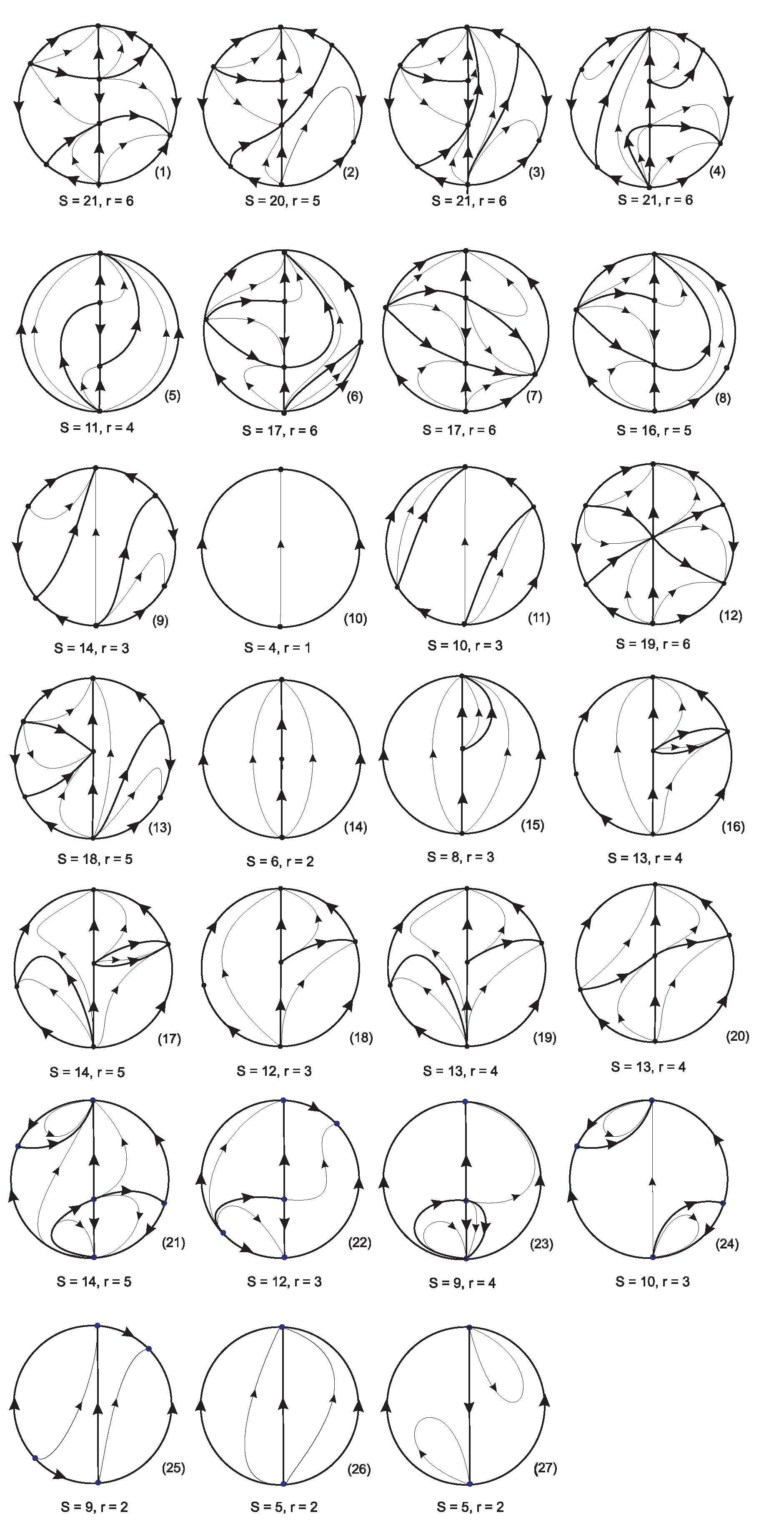
Figure 8.
The sequences of blow-ups for obtaining the local phase portrait at the origin of the local chart when , and .
Figure 8.
The sequences of blow-ups for obtaining the local phase portrait at the origin of the local chart when , and .
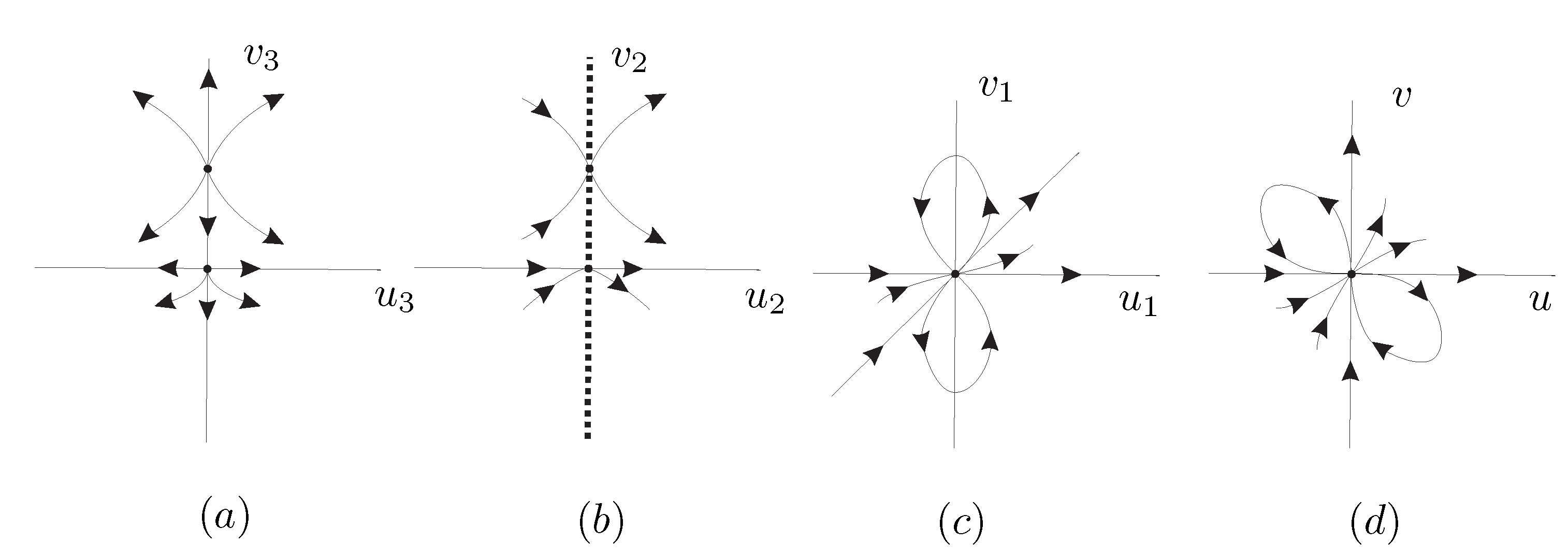
Figure 9.
The distinct topological local phase portraits at the origin of the local chart .
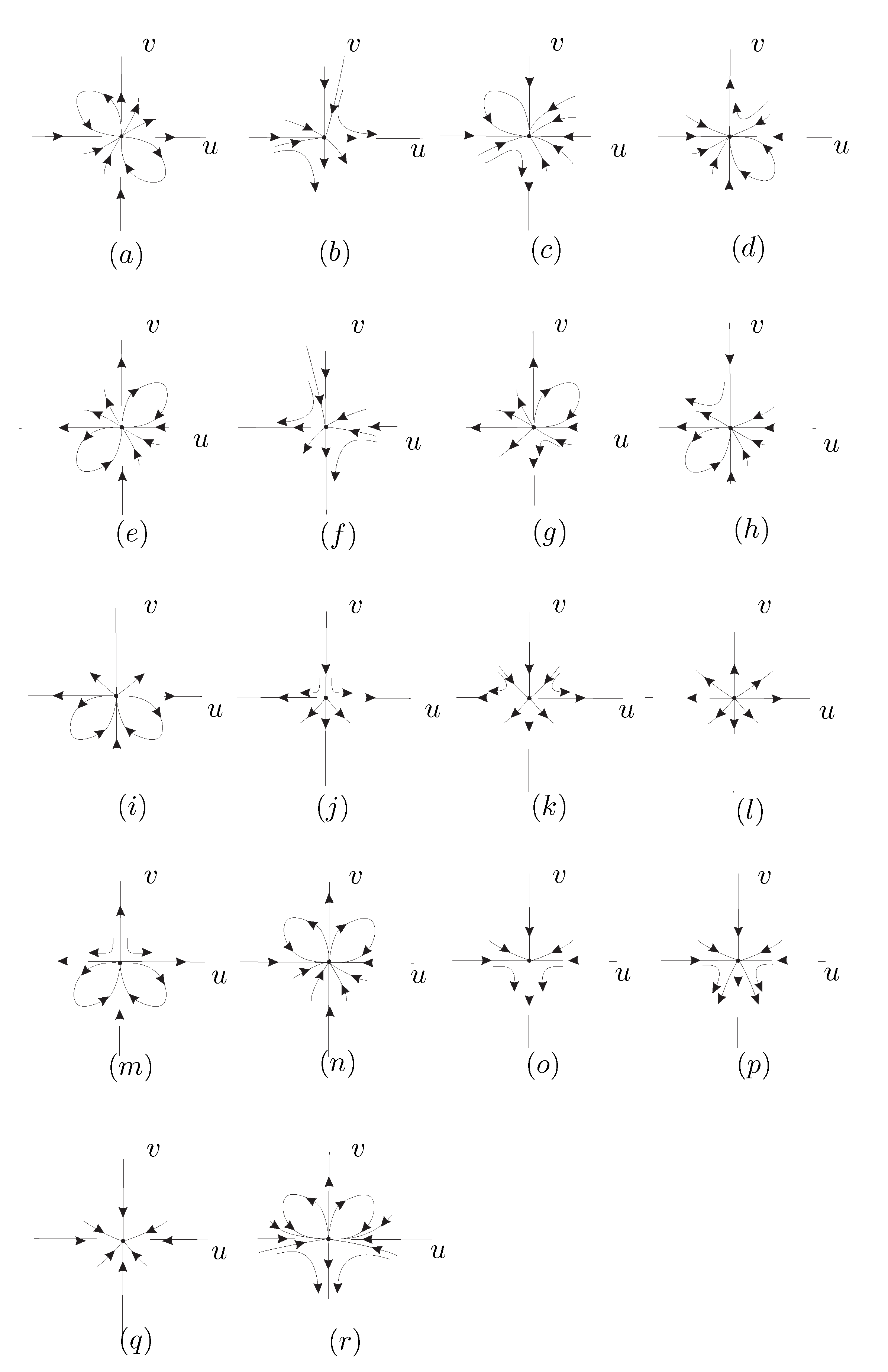
Figure 10.
The local phase portraits at the finite and infinite singular points for the case , and .
Figure 10.
The local phase portraits at the finite and infinite singular points for the case , and .
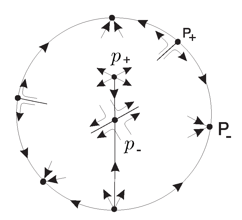
Figure 11.
All the distinct topological phase portraits of the quadratic systems VIII. Here s (respectively r) denotes the number of separatrices of a phase portrait in the Poincaré disc (respectively canonical regions).
Figure 11.
All the distinct topological phase portraits of the quadratic systems VIII. Here s (respectively r) denotes the number of separatrices of a phase portrait in the Poincaré disc (respectively canonical regions).
Disclaimer/Publisher’s Note: The statements, opinions and data contained in all publications are solely those of the individual author(s) and contributor(s) and not of MDPI and/or the editor(s). MDPI and/or the editor(s) disclaim responsibility for any injury to people or property resulting from any ideas, methods, instructions or products referred to in the content. |
© 2023 by the authors. Licensee MDPI, Basel, Switzerland. This article is an open access article distributed under the terms and conditions of the Creative Commons Attribution (CC BY) license (http://creativecommons.org/licenses/by/4.0/).
Copyright: This open access article is published under a Creative Commons CC BY 4.0 license, which permit the free download, distribution, and reuse, provided that the author and preprint are cited in any reuse.