Submitted:
30 June 2023
Posted:
03 July 2023
You are already at the latest version
Abstract
Protein molecules show varying degrees of flexibility throughout their three-dimensional structures. This flexibility is associated with the fluctuation of the torsion angle in proteins. The protein backbone can be defined mainly by two torsion angles, phi (φ) and psi (ψ). The fluctuation of torsion angles is derived from different NMR models’ variations in backbone torsion angles. The angle fluctuations in the cartesian coordinate space are used to characterize the protein’s structural flexibility. Fluctuation of torsion angle is useful in predicting protein function and structure when the torsion angles are used as restraints. This study aims to develop a machine learning method to predict torsion angle fluctuations directly from protein sequences. It explores various useful features such as disorder probability, position-specific scoring matrix profiles, secondary structure probabilities, monograms, bigram, position-specific estimated energy, half-sphere exposures, etc. Likewise, it explores well-known machine learning methods and proposes an optimized Light Gradient Boosting Machine Regressor (LightGBM) method, named TAFPred, to predict torsion angle fluctuations with the selected features. The proposed method achieves ten-fold cross-validated correlation coefficients of 0.746 and 0.737 and mean absolute errors of 0.114 and 0.123 for the angle fluctuation of φ and ψ, respectively, and attains an improvement of 10.08% in MAE, 24.83% in PCC in the phi angle, and 9.93% in MAE, 22.37% in PCC in psi angle compared to the state-of-the-art method proposed by Zhang et al.
Keywords:
backbone torsion angle
; torsion angle fluctuations
; machine learning
1. Introduction
Protein is an organic molecule of carbon, hydrogen, nitrogen, oxygen, and sulfur [1]. The core carbon atom is coupled to a side chain group, an amine group, a carbonyl group, and a hydrogen atom [2] to form a protein molecule. Protein molecules are essential and comprise many structures and functions within the cell. They also play an important role in the cell, forming many structures and performing numerous functions [3]. Protein molecules, such as actin and tubulin, can be structural and help shape the cell. They can also be functional, such as enzymes that perform critical metabolic reactions. A protein’s tertiary structure refers to how it folds in space in three dimensions. The polypeptide chain may require the assistance of chaperone proteins after it is synthesized at the ribosome [4,5]. The chaperone proteins also form temporary hydrogen bonds with the polypeptide chain, encouraging it to take the proper shape. This enables proper folding and, as a result, proper protein function. Some protein molecules do not fold to their native state and remain in a flexible state. Protein structural flexibility enables several types of dynamic and functional motions which are essential for interactions between proteins and peptides, DNA, RNA, or carbohydrate.
Protein structure can be illustrated by backbone torsion angles (Figure 1): rotational angles about the N-Cα bond (φ) and the Cα-C bond (ψ) or the angle between Cαi-1-Cαi-Cαi + 1 (θ) and the rotational angle about the Cαi-Cαi + 1 bond (τ) [6]. Prediction of Cα atom-based angle has demonstrated their potential usefulness in model quality assessment and structure prediction [7,8].
Several methods have been developed to predict backbone torsion angles. Angle predictions have been shown to be useful in fold recognition [9, 10] and fragment-based [11] or fragment-free structure prediction [12]. ANGLOR [13] utilizes support vector machines and neural networks for predicting the value of φ and ψ separately. TANGLE [14] uses a support vector regression method to predict backbone torsion angles (φ, ψ). Li et al. [15] predicted protein torsion angles by using four deep learning architectures, consisting of a deep neural network (DNN), a deep restricted Boltzmann machine (DRBN), and a deep recurrent neural network (DRNN), and a deep recurrent restricted Boltzmann machine (DReRBM). In addition, Heffernan et al. [7] captured the nonlocal interactions and yielded the highest reported accuracy in angle prediction by using long short-term memory bidirectional recurrent neural networks. A good prediction of angle probability may provide significant information on structural flexibility and intrinsic protein disorder in the extreme scenario [14]. In recent times, there have been notable advancements in the field of protein structure prediction using deep learning techniques. Specifically, AlphaFold [16], OmegaFold [17], and ESMFold [18] have demonstrated remarkable performance in predicting the three-dimensional (3D) structure of structured proteins. However, it should be noted that these methods excel primarily in predicting structured proteins [16]. On the contrary, the prediction of Phi and Psi angle fluctuations holds the potential for aiding in the prediction of unstructured or disordered protein structures.
However, to the best of our knowledge, only one research [19] presents work on backbone torsion angle fluctuation which is derived from the variation of backbone torsion angles. Because most proteins lack a known structure, the need for locating flexible (potentially functional) regions of a protein is the driving force behind the sequence-based prediction of torsion angle fluctuation. Moreover, using predicted torsion angles and flexibility as restraints can aid in protein structure and disordered region predictions. So, there is a dire need to improve the existing method to predict torsion angle fluctuations from protein sequences. The only method we found is developed by Zhang et al. [19]. They represented a neural network method for backbone torsion angle fluctuation based on sequence information only. Their model achieved ten-fold cross-validated correlation coefficients of 0.59 and 0.60 and the mean absolute errors (MAEs) of 22.7° and 24.3° for the angle fluctuation of φ and ψ, respectively.
In this work, we developed a machine learning method [20], TAFPred, to predict the backbone torsion angle fluctuation. Various features are directly extracted from protein sequences. A sliding window is used to include information from the neighbor residues. Furthermore, in TAFPred, we utilize a genetic algorithm (GA)-based feature selection method to extract several relevant features from the protein sequence. Finally, we train an optimized Light Gradient Boosting Machine to predict the backbone torsion angle fluctuation. We believe this is the second work that presents a sequence-based prediction method for backbone torsion angle fluctuation. We hope it will help further the protein structure and protein disorder prediction.
2. Materials and Methods
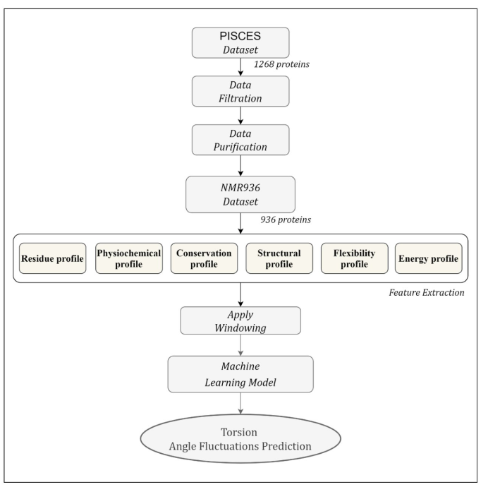
This section describes the dataset, feature extraction method, performance evaluation metrics, feature window selection, and finally, we describe the selected method for training the model. Figure 2 shows the workflow of the proposed TAFPred method.
2.1. Dataset
We collected 1268 protein chains from the author [19]. The protein chains are determined by the Nuclear Magnetic Resonance (NMR) method from the precompiled CulledPDB lists by PISCES using a sequence identity threshold of 25%. 997 protein chains are selected [19] by removing the chains with less than 5 NMR models, smaller than 25 amino acids, and consisting of nonstandard amino acid types. Finally, 936 protein chains are obtained by removing chains for which feature could not be obtained (referred to as NMR936) [21]. The backbone torsion angle fluctuation is derived from the variation of backbone torsion angles from different NMR models.
2.2. Feature extraction
We extracted several relevant profiles from the protein sequences, i.e., the Residue profile, Conservation profile, Physiochemical profile, Structural profile, and Flexibility profile. Here we briefly describe each of the profiles.
Residue profile. Twenty different numerical values are used to represent 20 standard amino acids (AA) types, yielding one feature per amino acid. The importance of this feature in solving bioinformatics problems has been shown in previous studies [22,23,24].
Physiochemical profile. In this work, five highly compact numeric patterns reflecting polarity, secondary structure, molecular volume, codon diversity, and electrostatic charge are extracted from [25] and used as features to represent the respective properties of each amino acid.
Conservation profile. The conservation profile of the protein sequence is obtained in terms of a normalized position-specific scoring matrix (PSSM) from the DisPredict2 program [24]. The PSSM is a matrix of L × 20 dimensions. The high scores suggest highly conserved locations, while scores around zero or negative indicate a less conserved position. The PSSM score was used to calculate monogram (MG) and bi-gram (BG) features. In terms of transition probabilities from one amino acid to another, the MG and BG properties can be used to characterize the portion of a protein sequence that can be conserved within a fold. From the DisPredict2 tool, we collect 1-D MG and 20-D BG characteristics.
Structural profile. Numerous biological problems have been solved using local structural features such as predicted secondary structure (SS) and accessible surface area (ASA) of amino acids. Here, the predicted ASA and SS probabilities for helix (H), coil (C), and beta-sheet (E) at the residue level is obtained from the DisPredict2 program. Moreover, we collect a separate set of SS probabilities for H, C, and E at the residue level from the BalancedSSP [26] program, as it provides a balanced prediction of these SS types. Thus, we extracted seven total structural properties (one ASA per amino acid and six predicted SS probabilities) as a structural profile of protein sequences.
Flexibility profile. Previous studies have demonstrated that an intrinsically disordered region (IDR) contains PTM sites, sorting signals and plays an important role in regulating protein structures and functions [27,28,29]. In this study, we used a disorder predictor named DisPredict2 [24] to accurately predict the protein’s disordered regions and obtain the disorder probability as a feature. To further improve the feature quality, we obtained two predicted backbone angle fluctuations, dphi (ΔΦ) and dpsi (ΔΨ), the DAVAR program [19].
Energy profile by Iqbal and Hoque [24], proposed a novel method that uses contact energy and predicted relative solvent accessibility (RSA) to estimate position-specific estimated energy (PSEE) of amino acid residues from sequence information alone. They showed that the PSEE could be used to distinguish between a protein’s structured and unstructured or intrinsically disordered regions. We utilized the PSEE score per amino acid as a feature in our study since it has been empirically demonstrated to have the ability to address a number of biological issues.
2.3. Machine Learning Methods
We analyzed the performance of eight individual regression methods: i) Light Gradient Boosting Machine Regressor (LightGBM) [30]; ii) Extreme Gradient Boosting Regressor (XGB) [31]; iii) Extra Tree Regressor (ET) [32]; iv) Decision Tree Regressor [33]; v) K-Nearest Neighbors Regressor [34,35]; vi) Convolutional Neural Network (CNN) [36]; and Long Short-Term Memory (LSTM) [37]; and Deep Neural Network (TabNet) [38]. The Light Gradient Boosting Machine Regressor (LightGBM) performs better, as shown in Table 2 and Table 3 under the Results Section.
2.4. Feature Selection Using Genetic Algorithm (GA)
We collected a feature vector of 179 dimensions (Figure 3) from different tools during the feature extraction process, which is significantly large. Therefore, to reduce the feature space and select the relevant features that could help improve the classification accuracy, we used a Genetic Algorithm (GA), a class of evolutionary algorithms, for feature selection. A detailed description of the feature selection approaches is provided below.
A GA is a population-based stochastic search technique that mimics the natural process of evolution. It contains a population of chromosomes, each representing a possible solution to the problem under consideration. In general, a GA operates by initializing the population randomly and iteratively updating the population through various operators, including elitism, crossover, and mutation, to discover, prioritize, and recombine good building blocks in parent chromosomes and finally obtain fitter ones [39,40,41].
Encoding the solution of the problem under consideration in the form of chromosomes and computing the fitness of the chromosomes are two important steps in setting up the GA. The length of the chromosome space is equal to the length of the feature space. Moreover, to compute the fitness of the chromosome, we use the LightGBM algorithm [33]. LightGBM was chosen because of its fast execution time and reasonable performance compared to other machine learning classifiers. During feature selection, the values of LightGBM parameters: max_depth, eta, silent, objective, num_class, n_estimators, min_child_weight, subsample, scale_pos_weight, tree_method, and max_bin were set to 6, 0.1, 1, ‘multi:softprob’, 2, 100, 5, 0.9, 3, ‘hist’ and 500, respectively and the rest of the parameters were set to their default value. The values of the LightGBM parameters mentioned above were identified through the hit-and-trial approach. In our implementation, the objective fitness is defined as:
2.5. Performance evaluation
The performances of all the machine learning methods have been examined using a 10-fold cross-validation approach with the evaluation metric shown in Table 1. We measure the performance of torsion angle fluctuation predictions by calculating the Pearson Correlation Coefficient (PCC) and Mean Absolute Error (MAE) with the following equations:
3. Results
In this section, we first show the performance of different machine learning methods. Then, we present the performance of the best model with optimized hyperparameters. Next, we present the applied sliding window technique results to find the optimum window size. Finally, we compared the proposed method with the state-of-the-art method.
3.1. Comparison between different methods
We experimented with eight machine learning methods. The performance comparison of the individual regressors on the training dataset for phi angle fluctuation is shown in Table 2. Most of the methods perform better than the state-of-the-art method [19] except Decision Tree Regressor. Table 2 further shows that the LightGBM is the best-performing regressor among eight regressors implemented in our study in terms of mean absolute value (MAE) and Pearson correlation coefficient (PCC). Moreover, LightGBM improves by 6.59% and 24.50% in terms of MAE and PCC, respectively, compared to the existing method.

Table 2.
Results from different machine learning methods (Phi Angle).
| Methods / Metric | MAE | PCC | MAE (% imp.) |
PCC (% imp.) |
Average (% imp.) |
|---|---|---|---|---|---|
| State-of-the-art method [19] | 0.126 | 0.598 | - | - | - |
| Extra Trees Regressor | 0.122 | 0.741 | 3.57% | 23.88% | 13.73% |
| XGB Regressor | 0.123 | 0.727 | 2.67% | 21.57% | 12.12% |
| KNN Regressor | 0.129 | 0.681 | -2.30% | 13.89% | 5.79% |
| Decision Tree Regressor | 0.167 | 0.527 | -24.38% | -11.84% | -18.11% |
| LSTM | 0.125 | 0.678 | 1.13% | 13.35% | 7.24% |
| CNN | 0.166 | 0.608 | -24.21% | 1.68% | -11.27% |
| Tabnet | 0.117 | 0.736 | 7.26% | 23.09% | 15.18% |
| LightGBM Regressor | 0.118 | 0.745 | 6.59% | 24.50% | 15.54% |
Best score values are boldfaced. Here, ‘imp.’ stands for improvement. The ‘% imp.’ represents the improvement in percentage achieved by TAFPred compared to the state-of-the-art method. Likewise, the ‘Average (% imp.)’ represents the average percentage improvement achieved by TAFPred for both MAE and PCC. Additionally, ‘(-)’ denotes that the % imp. or (Average % imp.) cannot be calculated.
Table 3 compares the individual regressors’ performance for psi angle fluctuations. We also found that the LightGBM regressor performs best than other methods. LightGBM attains an MAE of 0.127 and PCC of 0.733. Moreover, The LightGBM Regressor improves by 6.59% and 24.50% in terms of MAE and PCC, respectively, compared to the state-of-the-art method.
Table 3.
Results from different machine learning methods (Psi Angle).
| Methods / Metric | MAE | PCC | MAE (% imp.) |
PCC (% imp.) |
Average (% imp.) |
|---|---|---|---|---|---|
| State-of-the-art method [19] | 0.135 | 0.602 | - | - | - |
| Extra Trees Regressor | 0.131 | 0.729 | 2.77% | 21.10% | 11.94% |
| XGB Regressor | 0.132 | 0.715 | 2.22% | 18.73% | 10.48% |
| KNN Regressor | 0.139 | 0.670 | -2.63% | 11.24% | 4.31% |
| Decision Tree Regressor | 0.179 | 0.511 | -24.65% | -15.11% | -19.88% |
| LSTM | 0.132 | 0.665 | 2.29% | 10.48% | 6.38% |
| CNN | 0.144 | 0.702 | -6.46% | 16.61% | 5.07% |
| Tabnet | 0.126 | 0.724 | 7.24% | 20.28% | 13.76% |
| LightGBM Regressor | 0.127 | 0.733 | 6.09% | 21.84% | 13.96% |
Best score values are boldfaced. Here, ‘imp.’ stands for improvement. The ‘% imp.’ represents the improvement in percentage achieved by TAFPred compared to the state-of-the-art method. Likewise, the ‘Average (% imp.)’ represents the average percentage improvement achieved by TAFPred for both MAE and PCC. Additionally, ‘(-)’ denotes that the % imp. or (Average % imp.) cannot be calculated.
3.2. Hyperparameters optimization
We optimized the LightGBM Regressor parameters: learning_rate, estimators, max_depth, num_leaves, max_bin, feature_fraction, etc., to achieve the best 10-fold cross-validation performance and for sampling hyperparameters and pruning efficiently unpromising trials. We have used the custom objective function as PCC+(1-MAE) for optimization. The best values of the parameters: learning_rate, estimators, max_depth, num_leaves, max_bin, and feature_fraction were found to be 0.014, 2561, 19, 380, 138, and 0.52, respectively.
3.3. Feature window selection
Here, we applied a widely used feature windowing technique to include the neighboring residue features. We examined a suitable sliding window size that determines the appropriate number of residues around a target residue that helps the model attain improved performance. We designed several models with different window sizes (ws) (1, 3, 5, and so on). We used the following custom metric as the objective function to measure the performance.
Figure 4 shows the performance of the optimized LightGBM regressor for different window sizes for the Phi angle. The LightGBM regressor slightly improves window size 3, and the performance gradually decreases.
Figure 5 shows the performance of the optimized LightGBM regressor for different widow sizes for psi angle. The LightGBM regressor performance improves for window size 3, and then the performance gradually decreases. So, we select window size 3 to train the final model.
3.4. Comparison with the State-of-the-art method
Here, we compare the performance of the proposed method, TAFPred, with an existing state-of-the-art method [19] proposed by Zhang et al.. Table 4 shows that our proposed method improves by 10.08% in MAE, and 24.83% in PCC in the phi angle compared to the state-of-the-art method [19].
Table 5 shows that our proposed method improves by 9.93% in MAE and 22.37% in PCC in psi angle compared to the state-of-the-art method. Our proposed method significantly outperforms the existing state-of-the-art method and can more accurately predict the protein’s backbone torsion angle fluctuations.
4. Discussion
In this section, we explored diverse characteristics associated with the distribution of torsion-angle fluctuation. We examined the correlation between Δφ and Δψ, as well as the connection between torsion-angle fluctuation and disordered regions, utilizing our newly generated dataset.
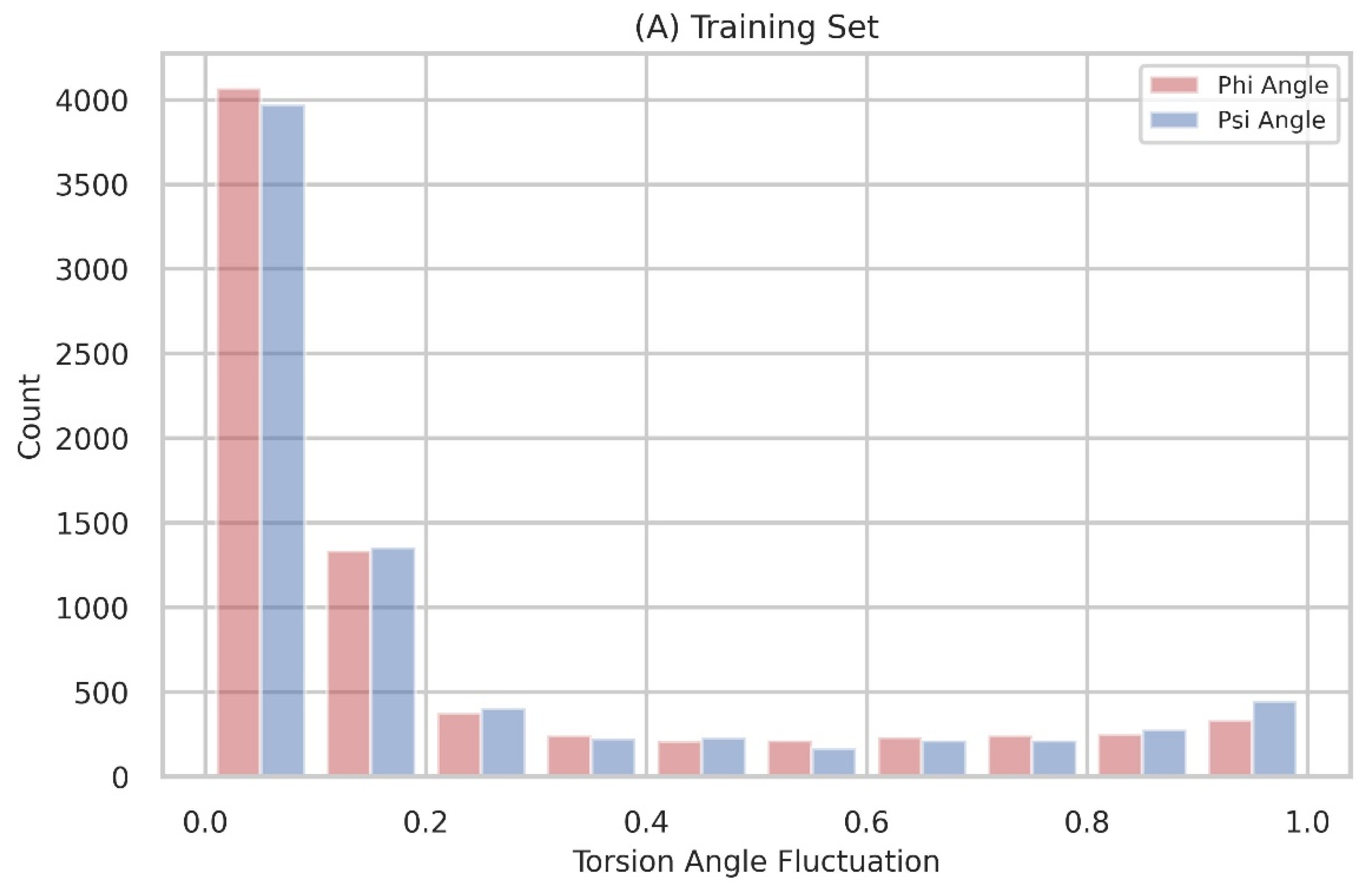
The distribution of torsion-angle fluctuation
Figure 1 displays the distribution of torsion-angle fluctuation, with the dataset divided into 10 bins. The distributions are non-uniform, and the majority of residues exhibit angle fluctuations below 0.2. This observation indicates that stable protein structures are characterized by a limited presence of flexible residues.
Figure 6.
The torsion-angle fluctuation is depicted in its distribution, with the data points divided into 10 bins. The fluctuations of the phi and psi angles are visually represented using red and green colors, respectively.
Figure 6.
The torsion-angle fluctuation is depicted in its distribution, with the data points divided into 10 bins. The fluctuations of the phi and psi angles are visually represented using red and green colors, respectively.
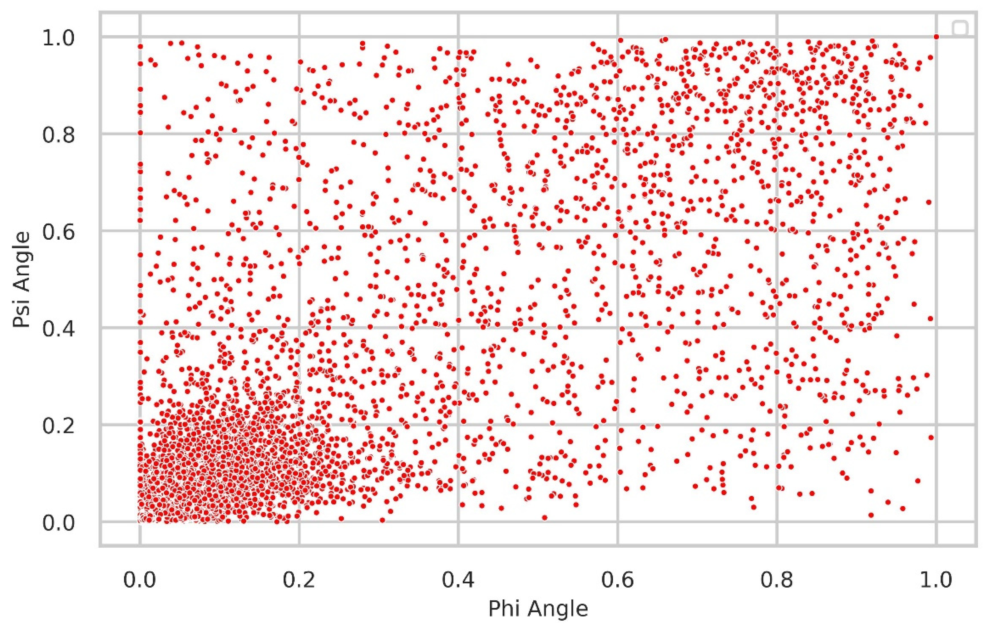
Relationship between Δφ and Δψ
We further examined the relationship between the Δφ and Δψ angles, which represent the fluctuation of neighboring rotational angles in the protein backbone for the same residue. A chemical bond linkage results in a correlation between these angles, as it is impossible to alter one torsion angle without affecting the other. Consequently, a notable and significant correlation was observed between them. Consistently, the majority of residues exhibited minimal fluctuations below 0.2, as anticipated.
Figure 7.
The relationship between Δφ and Δψ is shown in the figure, revealing that the majority of residues exhibit small fluctuations below 0.2.
Figure 7.
The relationship between Δφ and Δψ is shown in the figure, revealing that the majority of residues exhibit small fluctuations below 0.2.
Relationship between torsion-angle fluctuation and disordered regions
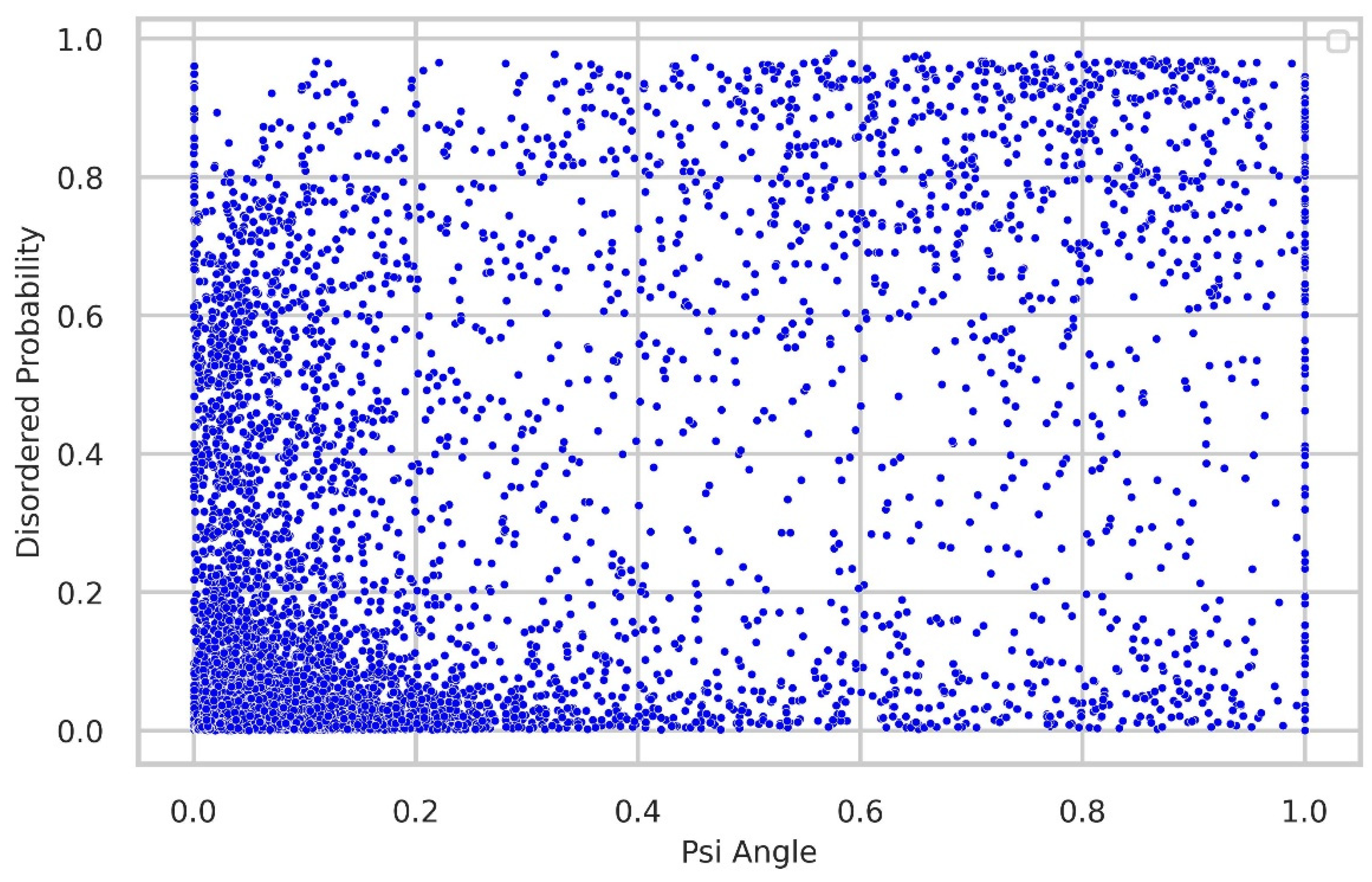
We thoroughly investigated the connection between torsion-angle fluctuation and disordered regions. To gather disordered probability data, we utilized the SPOT-Disordered2 method. The figures provide clear evidence of the close relationship between phi and psi angle fluctuations and the presence of disordered regions. In the majority of samples, regions with low fluctuations exhibit a low disordered probability, while regions with higher fluctuations display relatively higher disordered probability, as illustrated in Figure 8 and Figure 9.
Figure 8.
Relationship between torsion-angle fluctuation in the Phi angle and disordered regions. The disordered probability was obtained from the SPOT-Disordered2 tool. The figure illustrates that regions with low disordered probability exhibit correspondingly low fluctuations in the Phi angle, and conversely, regions with high disordered probability show higher fluctuations in the Phi angle.
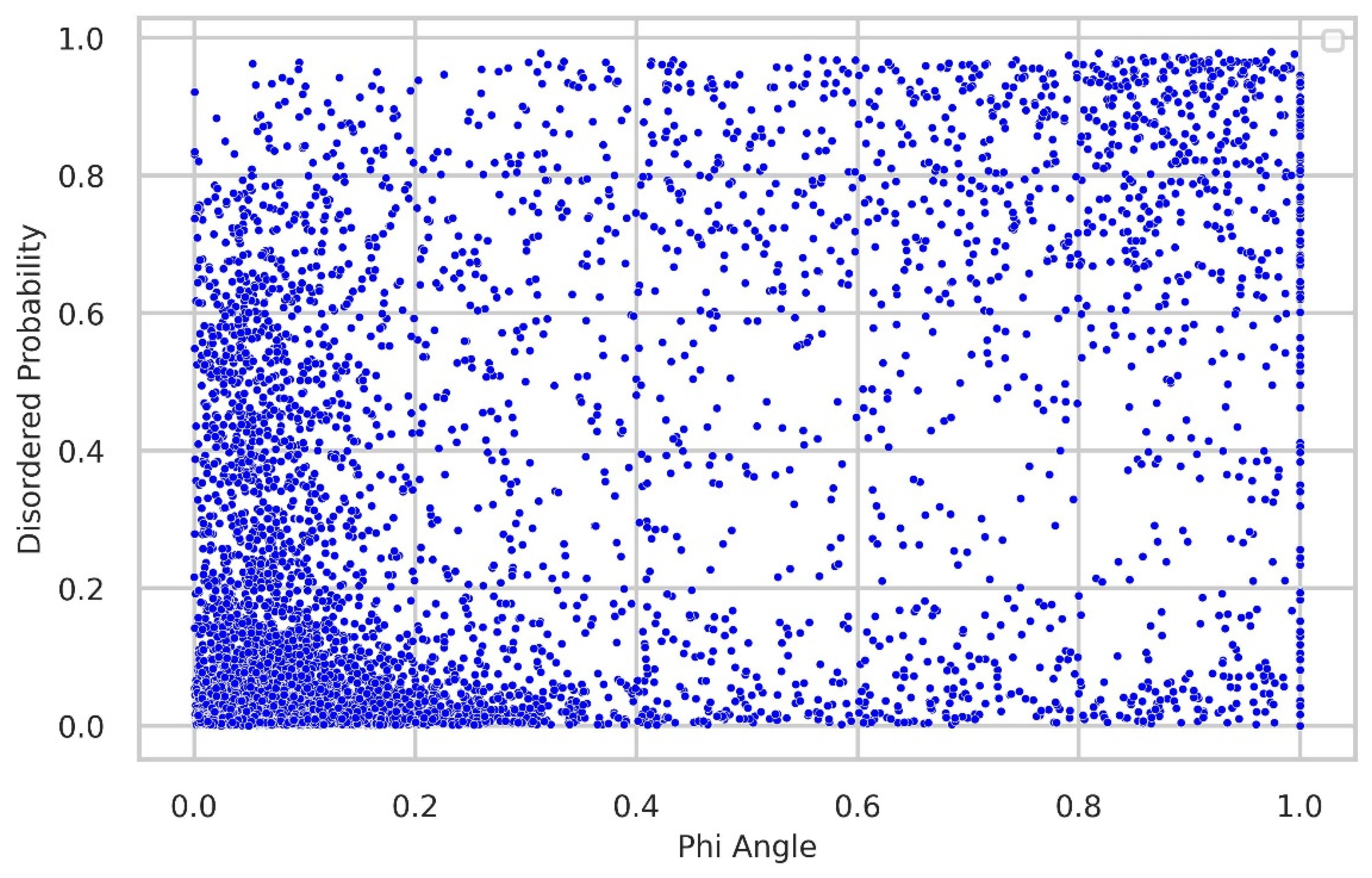
Figure 9.
Correlation between torsion-angle fluctuation in the Psi angle and the presence of disordered regions. The disordered probability was obtained through the utilization of the SPOT-Disordered2 tool. The figure clearly illustrates that regions with low disordered probability exhibit lower fluctuations in the Psi angle, while regions with high disordered probability tend to have higher fluctuations in the Psi angle.
5. Conclusions
In this study, we explored eight machine learning methods, including a recently published Deep Neural Network (TabNet) [1], and found that the Light Gradient Boosting Machine Regressor (LightGBM) performs best based on MAE and PCC. To optimize LightGBM Regressor, we used state-of-the-art sampling and pruning algorithms for hyperparameter tuning. Moreover, a custom objective function is used for optimization, and a sliding window technique is used to extract more information from the neighbor residues for improved performance. Our proposed method, TAFPred, shows an average improvement of 15.54% and 13.96% in both metrics (MAE and PCC) on phi and psi angles, respectively, compared to the state-of-the-art method [19]. In the future, we also plan to investigate the effect of torsion angle fluctuation in disorder proteins. We strongly believe the developed method will be helpful to the researcher in protein structure prediction and disordered prediction.
Author Contributions
Data collection and processing M.K. D.M.A., A.M., Conceived and designed the experiments: A.M., and M.T.H. Performed the experiments: M.K. Analysed the data: M.K., D.M.A. Contributed reagents/materials/analysis tools: M.T.H, Wrote the paper: M.K., D.M.A., A.M., and M.T.H. All authors have read and agreed on the publication of the final version of the manuscript.
Data Availability Statement
The code and data related to the development of TAFPred can be found here: https://github.com/wasicse/TAFPred.
Acknowledgments
A.M. would like to thank and acknowledge the generous support from the Department of Homeland Security (DHS) grant award 21STSLA00011-01-0. The authors also thank Dr. Yaoqi Zhou for publicly making the dataset available.
Conflicts of Interest
The authors declare no conflict of interest.
References
- Cornell WD, Cieplak P, Bayly CI, Gould IR, Merz KM, Ferguson DM, Spellmeyer DC, Fox T, Caldwell JW, Kollman PAJJotACS: A second generation force field for the simulation of proteins, nucleic acids, and organic molecules. 1995, 117(19):5179-5197.
- Nechab M, Mondal S, Bertrand MPJCAEJ: 1, n-Hydrogen-Atom Transfer (HAT) Reactions in Which n≠ 5: An Updated Inventory. 2014, 20(49):16034-16059.
- Wright PE, Dyson HJJJomb: Intrinsically unstructured proteins: re-assessing the protein structure-function paradigm. 1999, 293(2):321-331.
- Quiocho FAJArob: Carbohydrate-binding proteins: tertiary structures and protein-sugar interactions. 1986, 55(1):287-315.
- Mosimann S, Meleshko R, James MNJPS, Function,, Bioinformatics: A critical assessment of comparative molecular modeling of tertiary structures of proteins. 1995, 23(3):301-317.
- Gao J, Yang Y, Zhou Y: Grid-based prediction of torsion angle probabilities of protein backbone and its application to discrimination of protein intrinsic disorder regions and selection of model structures. BMC Bioinformatics 2018, 19(1):29. [CrossRef]
- Heffernan R, Yang Y, Paliwal K, Zhou Y: Capturing non-local interactions by long short-term memory bidirectional recurrent neural networks for improving prediction of protein secondary structure, backbone angles, contact numbers and solvent accessibility. Bioinformatics 2017, 33(18):2842-2849. [CrossRef]
- Lyons J, Dehzangi A, Heffernan R, Sharma A, Paliwal K, Sattar A, Zhou Y, Yang YJJocc: Predicting backbone Cα angles and dihedrals from protein sequences by stacked sparse auto-encoder deep neural network. 2014, 35(28):2040-2046.
- Yang Y, Faraggi E, Zhao H, Zhou YJB: Improving protein fold recognition and template-based modeling by employing probabilistic-based matching between predicted one-dimensional structural properties of query and corresponding native properties of templates. 2011, 27(15):2076-2082. [CrossRef]
- Karchin R, Cline M, Mandel-Gutfreund Y, Karplus KJPS, Function,, Bioinformatics: Hidden Markov models that use predicted local structure for fold recognition: alphabets of backbone geometry. 2003, 51(4):504-514.
- Rohl CA, Strauss CE, Misura KM, Baker D: Protein structure prediction using Rosetta. In: Methods in enzymology. vol. 383: Elsevier; 2004: 66-93. [CrossRef]
- Faraggi E, Yang Y, Zhang S, Zhou YJS: Predicting continuous local structure and the effect of its substitution for secondary structure in fragment-free protein structure prediction. 2009, 17(11):1515-1527. [CrossRef]
- Wu S, Zhang YJPo: ANGLOR: a composite machine-learning algorithm for protein backbone torsion angle prediction. 2008, 3(10):e3400.
- Yang Y, Gao J, Wang J, Heffernan R, Hanson J, Paliwal K, Zhou Y: Sixty-five years of the long march in protein secondary structure prediction: the final stretch? Brief Bioinform 2018, 19(3):482-494.
- Li H, Hou J, Adhikari B, Lyu Q, Cheng JJBb: Deep learning methods for protein torsion angle prediction. 2017, 18(1):1-13.
- Jumper J, Evans R, Pritzel A, Green T, Figurnov M, Ronneberger O, Tunyasuvunakool K, Bates R, Žídek A, Potapenko A et al: Highly accurate protein structure prediction with AlphaFold. Nature 2021, 596(7873):583-589.
- Wu R, Ding F, Wang R, Shen R, Zhang X, Luo S, Su C, Wu Z, Xie Q, Berger B et al: High-resolution de novo structure prediction from primary sequence. bioRxiv 2022.
- Lin Z, Akin H, Rao R, Hie B, Zhu Z, Lu W, Santos Costa Ad, Fazel-Zarandi M, Sercu T, Candido S et al: Language models of protein sequences at the scale of evolution enable accurate structure prediction. bioRxiv 2022:2022.2007.2020.500902.
- Zhang T, Faraggi E, Zhou Y: Fluctuations of backbone torsion angles obtained from NMR-determined structures and their prediction. Proteins 2010, 78(16):3353-3362. [CrossRef]
- Kabir MWU, Alawad DM, Mishra A, Hoque MT: Prediction of Phi and Psi Angle Fluctuations from Protein Sequences In: Accepted for 20th IEEE Conference on Computational Intelligence in Bioinformatics and Computational Biology: 2023; Eindhoven, The Netherlands.
- Md Kauser A, Avdesh M, Md Tamjidul H: TAFPred: An Efficient Torsion Angle Fluctuation Predictor of a Protein from its Sequence. In.; 2018.
- Iqbal S, Mishra A, Hoque T: Improved Prediction of Accessible Surface Area Results in Efficient Energy Function Application. Journal of Theoretical Biology 2015, 380:380-391. [CrossRef]
- Iqbal S, Hoque MT: PBRpredict-Suite: a suite of models to predict peptide-recognition domain residues from protein sequence. Bioinformatics 2018:bty352-bty352.
- Iqbal S, Hoque MT: Estimation of position specific energy as a feature of protein residues from sequence alone for structural classification. PLOS ONE 2016, 11(9):e0161452.
- Zhu L, Yang J, Song JN, Chou KC, Shen HB: Improving the accuracy of predicting disulfide connectivity by feature selection. Computational Chemistry 2010, 31(7):1478-1485. [CrossRef]
- Islam MN, Iqbal S, Katebi AR, Hoque MT: A balanced secondary structure predictor Journal of Theoretical Biology, 2016, 389:60–71. [CrossRef]
- Wright PE, Dyson HJ: Intrinsically unstructured proteins: re-assessing the protein structure-function paradigm. Journal of Molecular Biology 1999, 293(2):321-331. [CrossRef]
- Liu J, Tan H, Rost B: Loopy proteins appear conserved in evolution. Journal of Molecular Biology 2002, 322(1):53-64. [CrossRef]
- Tompa P: Intrinsically unstructured proteins. Trends in Biological Sciences 2002, 27(10):527-533. [CrossRef]
- Ho TK: Random decision forests. In: Document Analysis and Recognition, 1995, Proceedings of the Third International Conference on; Montreal, Que., Canada. IEEE 1995: 278-282.
- Breiman L: Bagging predictors. Machine Learning 1996, 24(2):123-140.
- Geurts P, Ernst D, Wehenkel L: Extremely randomized trees. Machine Learning 2006, 63(1):3-42. [CrossRef]
- Chen T, Guestrin C: XGBoost: a scalable tree boosting system. In: Proceedings of the 22Nd ACM SIGKDD International Conference on Knowledge Discovery and Data Mining. New York, NY, USA: ACM; 2016: 785-794.
- Hastie T, Tibshirani R, Friedman J: The Elements of Statistical Learning, 2 edn: Springer-Verlag New York; 2009.
- Szilágyi A, Skolnick J: Efficient prediction of nucleic acid binding function from low-resolution protein structures. Journal of Molecular Biology 2006, 358(3):922-933. [CrossRef]
- Altman NS: An Introduction to Kernel and Nearest-Neighbor Nonparametric Regression. The American Statistician 1992, 46:175-185.
- Ke G, Meng Q, Finley T, Wang T, Chen W, Ma W, Ye Q, Liu T-Y: LightGBM: a highly efficient gradient boosting decision tree. In: Proceedings of the 31st International Conference on Neural Information Processing Systems; Long Beach, California, USA. Curran Associates Inc. 2017: 3149–3157.
- Arik SO, Pfister T: TabNet: Attentive Interpretable Tabular Learning. arXiv 2019. [CrossRef]
- Hoque MT, Iqbal S: Genetic algorithm-based improved sampling for protein structure prediction. International Journal of Bio-Inspired Computation 2017, 9(3):129-141.
- Hoque MT, Chetty M, Sattar A: Protein Folding Prediction in 3D FCC HP Lattice Model using Genetic Algorithm. In: IEEE Congress on Evolutionary Computation (CEC) Singapore; Singapore. 2007: 4138-4145.
- Hoque MT, Chetty M, Lewis A, Sattar A, Avery VM: DFS Generated Pkathways in GA Crossover for Protein Structure Prediction. Neurocomputing 2010, 73:2308-2316.
Figure 1.
Torsion angles phi (φ) and psi (ψ). The phi angle is the angle around the -N-CA- bond (where ‘CA’ is the alpha-carbon), and the psi angle is the angle around the -CA-C- bond.
Figure 1.
Torsion angles phi (φ) and psi (ψ). The phi angle is the angle around the -N-CA- bond (where ‘CA’ is the alpha-carbon), and the psi angle is the angle around the -CA-C- bond.
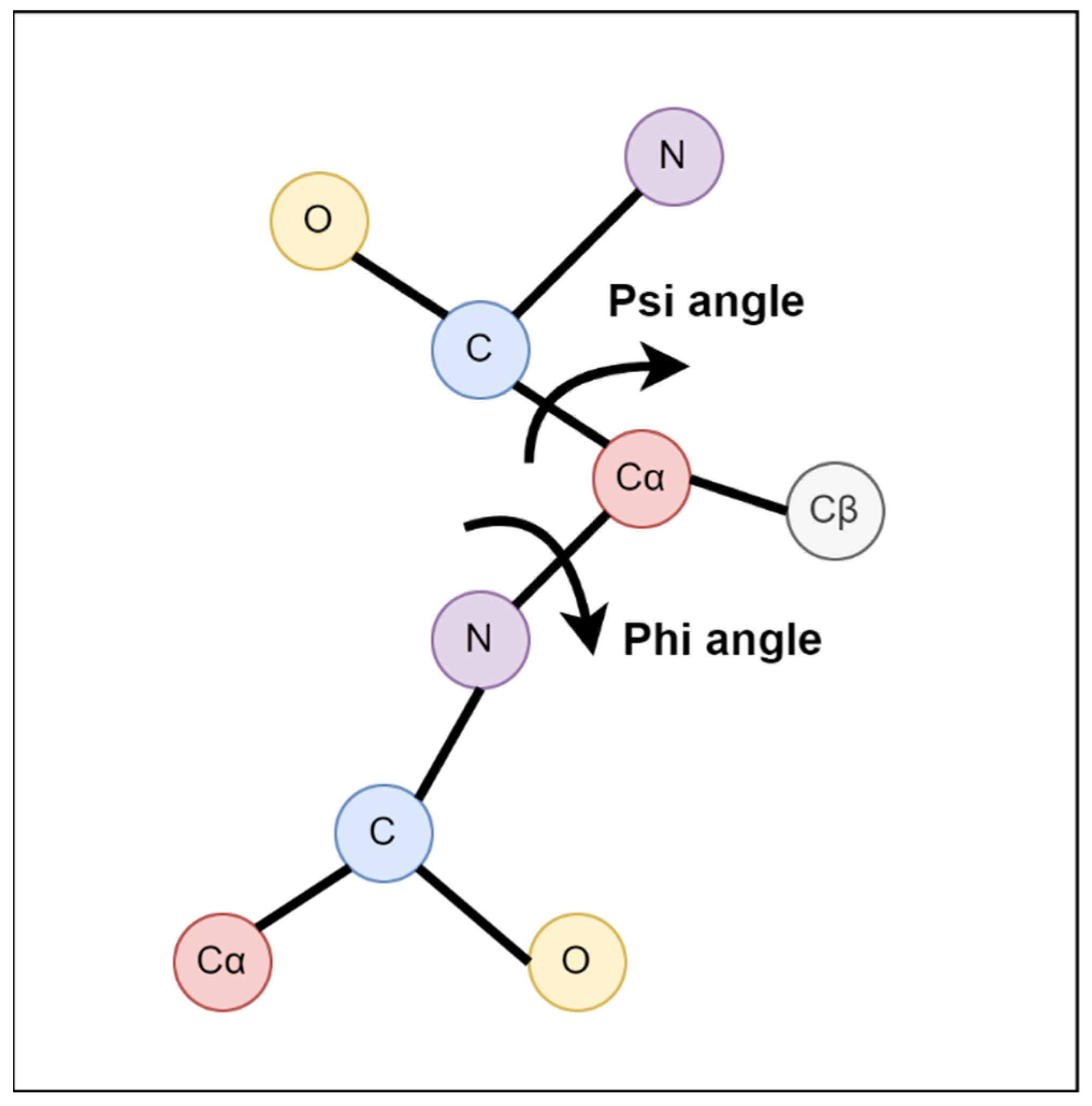
Figure 2.
Illustrates the workflow of the torsion angle fluctuation predictions.
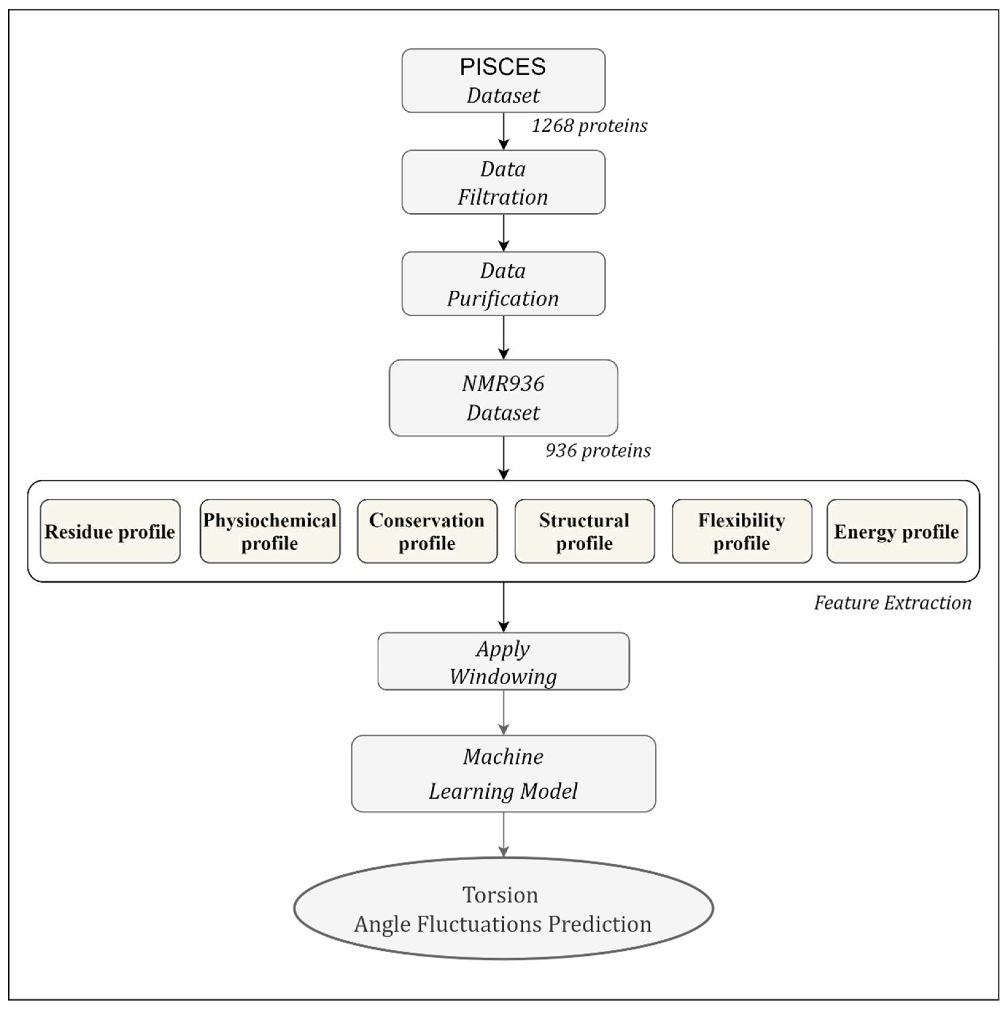
Figure 3.
Feature extraction from different tools.
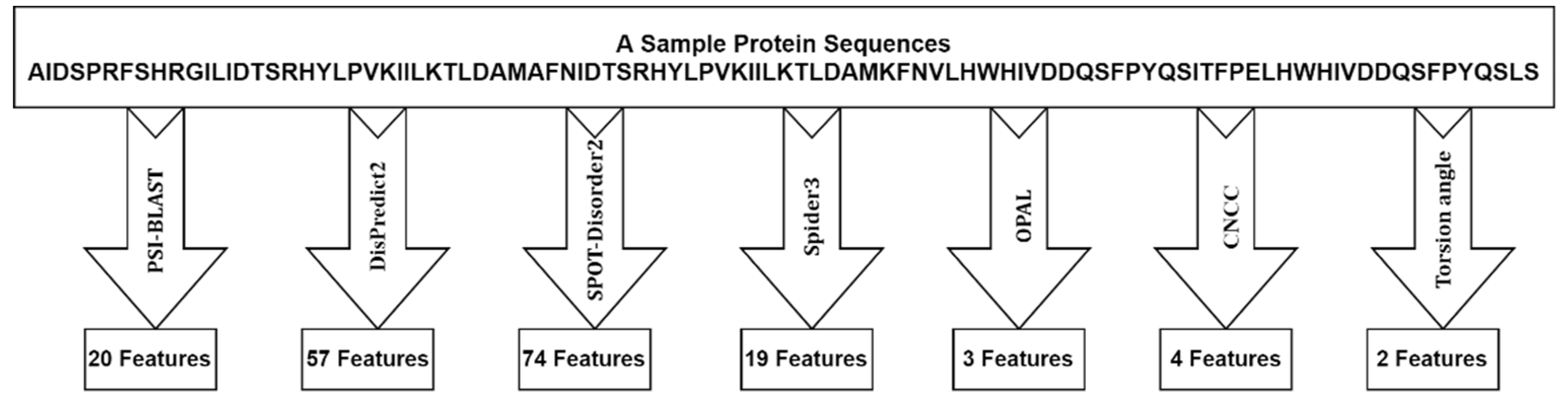
Figure 4.
Selection of sliding window size with Optimized LightGBM Regressor (Phi angle). Among the tested window sizes, it was found that a window size of 3 achieved the highest 1-MAE+PCC (Mean Absolute Error + Pearson Correlation Coefficient) for the Psi angle.
Figure 4.
Selection of sliding window size with Optimized LightGBM Regressor (Phi angle). Among the tested window sizes, it was found that a window size of 3 achieved the highest 1-MAE+PCC (Mean Absolute Error + Pearson Correlation Coefficient) for the Psi angle.
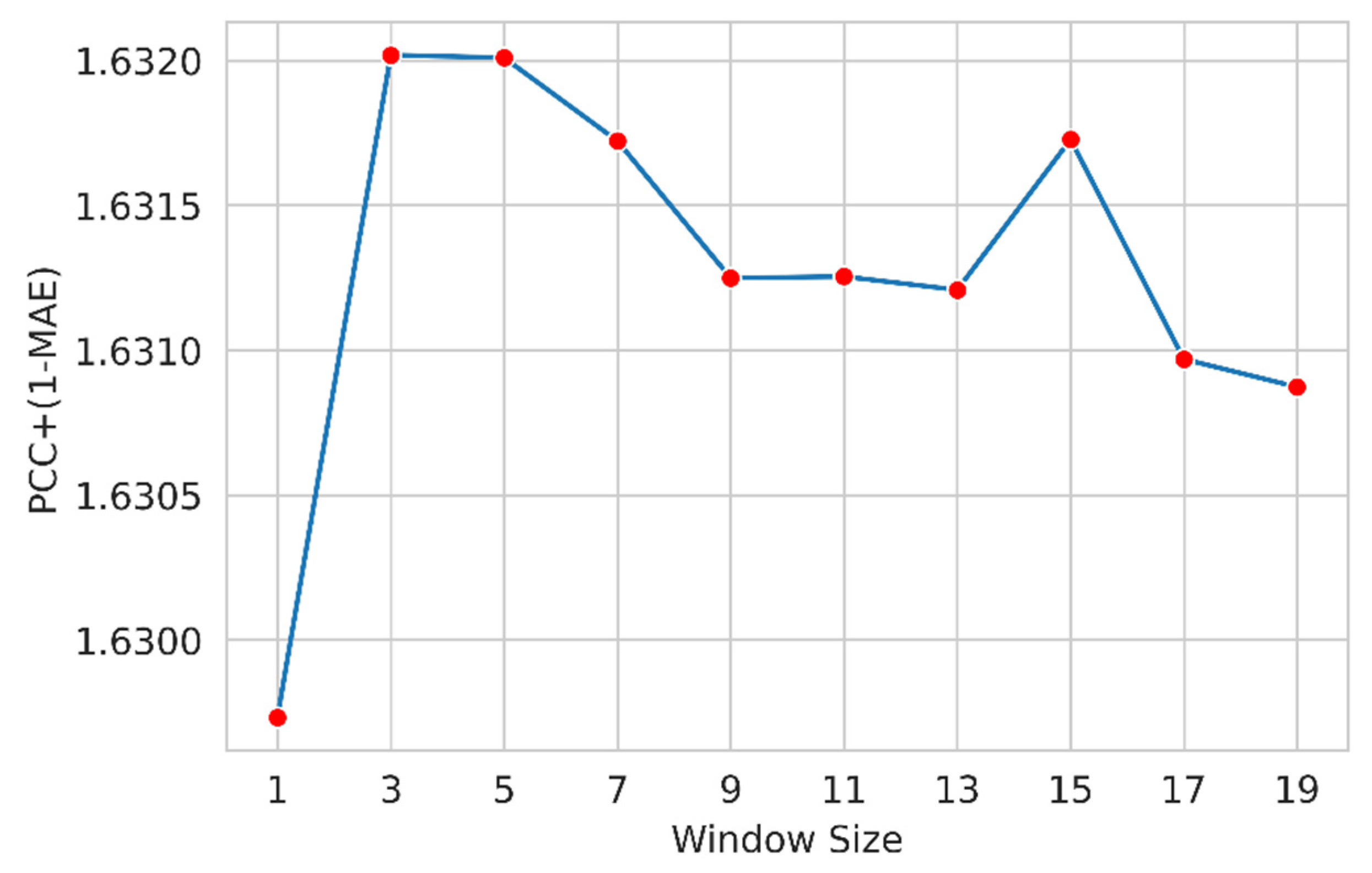
Figure 5.
Selection of sliding window size with Optimized LightGBM Regressor (Psi Angle). Among the tested window sizes, it was found that a window size of 3 yielded the highest value of 1-MAE+PCC for the Psi angle.
Figure 5.
Selection of sliding window size with Optimized LightGBM Regressor (Psi Angle). Among the tested window sizes, it was found that a window size of 3 yielded the highest value of 1-MAE+PCC for the Psi angle.

Table 1.
This is a table. Tables should be placed in the main text near the first time they are cited.
Table 1.
This is a table. Tables should be placed in the main text near the first time they are cited.
| Name of Metric | Definition |
|---|---|
| Pearson Correlation Coefficient (PCC) = | |
| Mean Absolute Error (MAE) = |
Here 𝑥𝑖 is the predicted torsion angle fluctuation, 𝑦𝑖 is the native torsion angle fluctuation for the i residue in the sequence, x̄ and ȳ are their corresponding sample means.
Table 4.
CV Results with Optimized LightGBM Regressor with sliding windows size 3 (Phi angle).
| Methods / Metric | MAE | PCC | MAE (% imp.) |
PCC (% imp.) |
Average (% imp.) |
|---|---|---|---|---|---|
| State-of-the-art method [19] | 0.126 | 0.598 | - | - | - |
| TAFPred | 0.114 | 0.746 | 10.08% | 24.83% | 17.45% |
Best score values are boldfaced. Here, ‘imp.’ stands for improvement. The ‘% imp.’ represents the improvement in percentage achieved by TAFPred compared to the state-of-the-art method. Likewise, the ‘Average (% imp.)’ represents the average percentage improvement achieved by TAFPred for both MAE and PCC. Additionally, ‘(-)’ denotes that the % imp. or (Average % imp.) cannot be calculated.
Table 5.
Cross-validation Results with sliding windows size 3 (Psi Angle).
| Methods / Metric | MAE | PCC | MAE (% imp.) |
PCC (% imp.) |
Average (% imp.) |
|---|---|---|---|---|---|
| State-of-the-art method [19] | 0.135 | 0.602 | - | - | - |
| TAFPred | 0.123 | 0.737 | 9.93% | 22.37% | 16.15% |
Best score values are boldfaced. Here, ‘imp.’ stands for improvement. The ‘% imp.’ represents the improvement in percentage achieved by TAFPred compared to the state-of-the-art [19] method. Likewise, the ‘Average (% imp.)’ represents the average percentage improvement achieved by TAFPred for both MAE and PCC. Additionally, ‘(-)’ denotes that the % imp. or (Average % imp.) cannot be calculated.
Disclaimer/Publisher’s Note: The statements, opinions and data contained in all publications are solely those of the individual author(s) and contributor(s) and not of MDPI and/or the editor(s). MDPI and/or the editor(s) disclaim responsibility for any injury to people or property resulting from any ideas, methods, instructions or products referred to in the content. |
© 2023 by the authors. Licensee MDPI, Basel, Switzerland. This article is an open access article distributed under the terms and conditions of the Creative Commons Attribution (CC BY) license (http://creativecommons.org/licenses/by/4.0/).
Copyright: This open access article is published under a Creative Commons CC BY 4.0 license, which permit the free download, distribution, and reuse, provided that the author and preprint are cited in any reuse.


