1. Introduction
As one of the sensors of autonomous vehicles’ environment perception, LiDAR is regarded as the "eye" with its advantages of high resolution, strong anti-interference ability, and high stability. MEMS LiDAR has promising technological development prospects due to its miniaturization, low power consumption, and low cost, and gradually becoming one of the main sensors for autonomous vehicles. As the vehicle moves, the LiDAR captures point cloud information from different perspectives of the target. Therefore, it is necessary to concatenate the front and rear frames to obtain the target's complete 3D point cloud information [
1].
Point cloud registration refers to matching and aligning source and target point clouds to maximize their overlap. Its core is to solve the spatial rotation and translation matrix between the source and target point cloud [
2]. Besl [
3] proposed a groundbreaking Iterative Closest Point (ICP) algorithm, The ICP has high registration accuracy but has harsh application conditions. Therefore, scholars from various countries had proposed a series of improved algorithms [
4,
5,
6,
7,
8,
9,
10].
In addition to ICP, Magnusson [
11] proposed the NDT algorithm. Aiger [
12] proposed the 4PCS algorithm. Theiler [
13] proposed the K4PCS algorithm, which first extracts key points using the 3D-Harris [
14] or 3D-DoG [
15] algorithms. Xu [
16] proposed a 4-Plane Congruent Set based on Voxel geometric constraint (V4PCS) algorithm for semi-automatic.
When point cloud data (PCD) have massive information, the feature-based coarse registration method is usually used. This method can only select special points for registration without the need for the initial pose, including feature description and extraction. Commonly used feature descriptors include PFH, FPFH, SHOT, 3DSC, CSF, RMF, 2D Line Features, and LPPF [
17,
18,
19,
20,
21,
22,
23]; Keypoint extraction algorithms include 3D DoG, 3D Harris, SIFT, Hough Transform, and RANSAC based plane detection [
24,
25,
26].
In recent years, new methods have been constantly emerging, and application scenes have been expanding [
27,
28,
29,
30,
31,
32,
33,
34]. Among them, an improved ICP algorithm combining RANSAC, ISS, and 3DSC is proposed in [
30]. In [
31], point features are extracted by calculating the FPFH, and RANSAC and ICP are used to search and align.
In outdoor environments, MEMS LiDAR may collect PCD with high noise and low overlap due to frequent changes in road conditions and vehicle speeds. Proposed a fast registration method for this. The method takes preprocessing, coarse registration, and fine registration as the main axis, and combined them with an improved voxel filter, keypoints extraction, and self-adaptive segmentation model (SSM). The effectiveness of the method on the PandaSet [
35] and The Real LiDAR-Derived PCD is verified. Compared with other algorithms, the new method is precise and efficient.
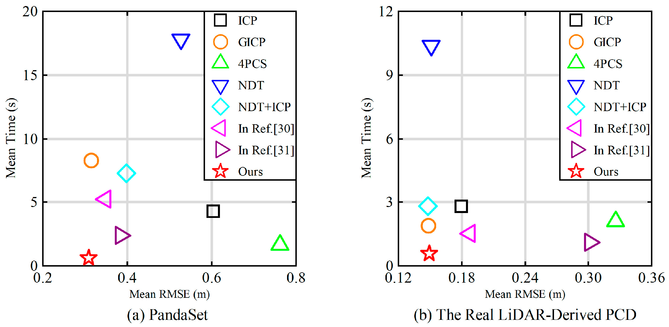
Figure 1.
Accuracy and runtime (The mean root mean square error (RMSE) and mean Time of different registration algorithms in PandaSet and The Real LiDAR-Derived PCD).
Figure 1.
Accuracy and runtime (The mean root mean square error (RMSE) and mean Time of different registration algorithms in PandaSet and The Real LiDAR-Derived PCD).
The remainder of this paper is as organized follows.
Section 2 provides the registration process and characteristics of the 4PCS and NDT algorithms.
Section 3 introduces the proposed algorithm's registration strategy, principle, and partial program flow. Next, the comparison results between our method and existing algorithms are presented in
Section 4. Finally,
Section 5 introduces the conclusions and future work.
2. Related Works
2.1. 4PCS Algorithm
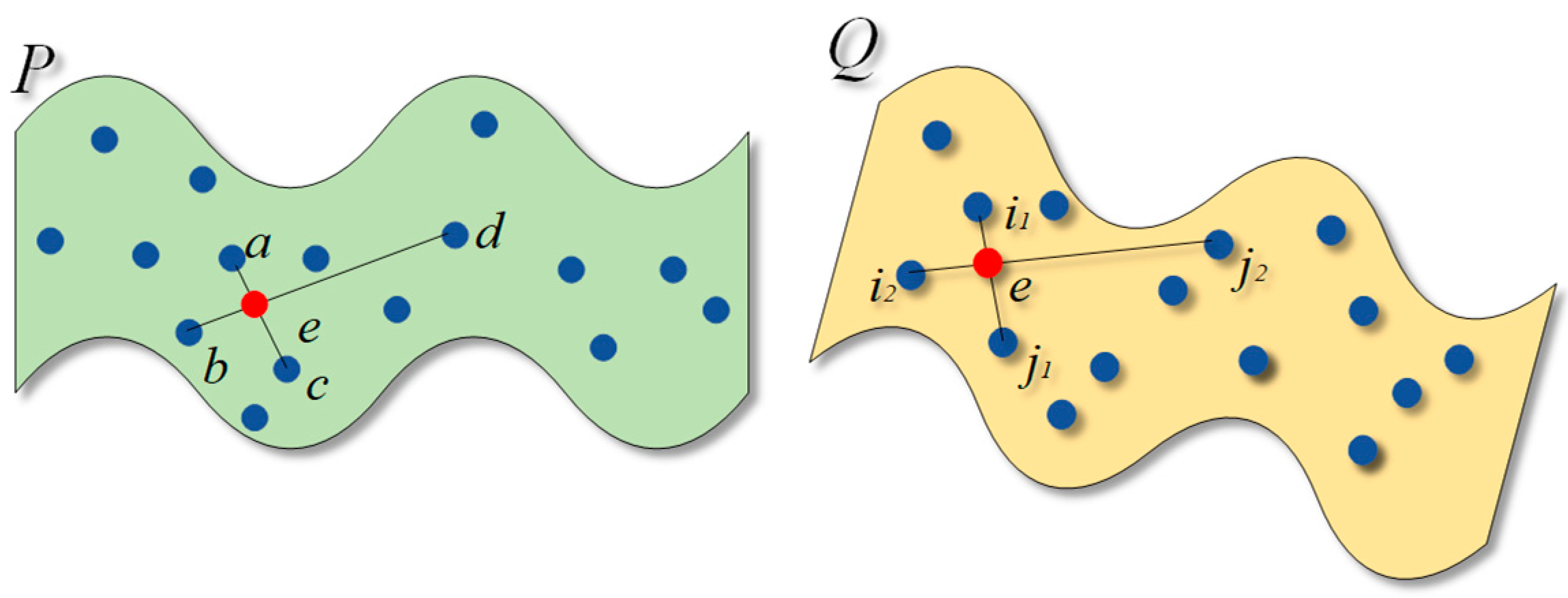
The 4PCS algorithm utilizes the principle of affine invariance to search for approximately identical coplanar 4-point sets in two frames and determines the optimal transformation matrix Tbest by calculating the degree of overlap.
Randomly select three points
a,
b, and
c to determine a plane, then select a point
d to form the plane
B ⊂
P. Let the line
ac intersect the line
bd at point
e, as shown in
Figure 2:
So, obtain two affine invariant ratios
R1 and
R2:
For any point-pair
i1,
j1∈
Q, calculate two intersections that conform to the affine ratio:
During the pairing process, approximately coplanar point sets are often used for matching, so it is necessary to eliminate point sets with significant differences.
If
Q is transformed by
Tk to
Q', and the distance between any point in
Q' and any point in
P is
d, then:
Where: qQ’, qP are any points in Q' and P, respectively, ε is the distance threshold of point-pairs.
If point cloud P and Q are in ε the set of 4-point sets paired within the range is D = {D1, ..., Dk}, calculate Tk between the plane pairs B, U within D. Allocate matching scores based on the number of point-pairs that comply with equation (3). When the score is the highest, Tbest = Tk.
To use 4PCS, three important parameters need to be provided: ε, the approximate overlap rate Or, and the target distance Dt. Compared to ICP, 4PCS does not require initial pose, has good anti-interference and a wide range of applications, and is usually used for coarse registration.
2.1. NDT Algorithm
Magnusson was inspired by the 2D-NDT [
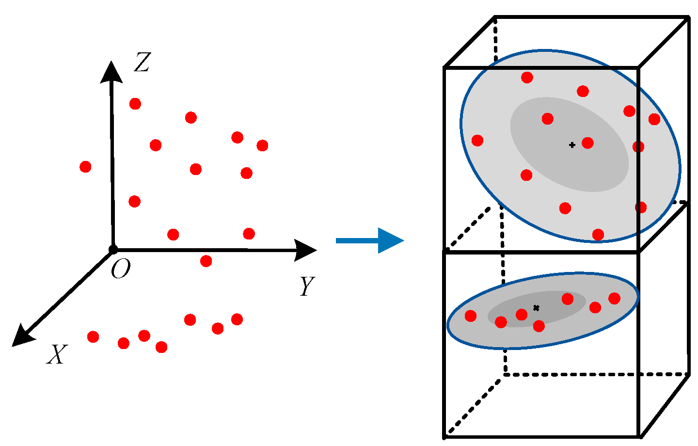
36] algorithm and expanded from 2D to 3D. Its core is to establish a continuous and differentiable probability density function (PDF) based on the normal distribution of 3D density. Thus, the solution of the transformation matrix is transformed into the optimization of continuous function. The schematic is shown in
Figure 3.
The steps of the NDT algorithm are as follows:
Step 1: Divide the space into blocks and place the target point cloud into blocks.
Step 2: Calculate the parameters, mean vector
and covariance matrix
Σ of the PDF, whose values are:
Where: m is the number of points within a block; is the scanning points of the target point cloud within the block; T is the transformation matrix.
Step 3: Initialize or update the transformation parameters and search for the corresponding block again.
Step 4: Calculate the PDF of the block:
Where: D = 3; is a Scan point within the source cloud.
Step 5: To obtain the optimal transformation matrix, maximize the likelihood function:
Where: represents transforming through .
Minimize the objective function
F(
), which is the negative logarithm of the likelihood function.
Step 6: Establish the score function gscore, use the Newton algorithm to minimize the gscore, and update the transformation.
Step 7: Finally, determine whether the updated amount is converging. If so, end. Otherwise, repeat steps 3 to 6.
NDT divides point cloud space into multiple small blocks for statistical calculation, which enables it to quickly process large-scale PCD and to some extent overcome the influence of noise and outliers.
3. Methodology
The method includes three parts: Preprocessing, Coarse registration, and Fine registration. See
Figure 3 for details.
Figure 4.
Architecture of the proposed method.
Figure 4.
Architecture of the proposed method.
In the preprocessing, pass-through filter and improved voxel filter are used to trim and simplify the point cloud; In the coarse registration, ISS is used to extract the keypoints, and then 4PCS is used to provide the initial attitude; In the fine registration, the SSM model based on the density characteristics of key points is constructed, and the model is embedded in NDT to complete the fine registration.
3.1. Preprocessing
To reduce noise interference, the input point cloud is first preprocessed. For PCD scanned by Vehicular mounted LiDAR, there are many outliers and isolated noise points at the edges. The pass-through filter can be used to crop edges. In addition, voxel filtering can effectively simplify input point clouds, reduce subsequent calculations, and retain shape features.
The improved voxel filter limits the minimum number of points on the original basis, which means that the number of points in each voxel grid must reach the minimum limit value
nmin, otherwise the size of voxel grids will be expanded. In addition, replace the voxel barycenter point
Pb with the closest point
Pv of the voxel barycenter:
Where: n is the number of points in the voxel grid, (xi, yi, zi) and (xb, yb, zb) are the coordinates of any point Pi and the voxel barycenter point Pb in the grid, respectively.
The changes of the voxel filter are shown in
Figure 5:
Compared with before improvements, the grid size is larger at the sparse place, improving the Downsampling accuracy and reducing the number of edge outliers. To prevent data bias and ensure registration accuracy, the filtering result now uses the closest point to the barycenter instead of the barycenter itself.
3.1. I4PCS Coarse Registration
ISS [
37] is an algorithm to describe the intrinsic shape characteristics of solid geometry, which can be used to extract keypoints from the point cloud. The idea of feature point detection is similar to Principal Component Analysis (PCA), which aims to reduce the dimensionality of high-dimensional data. The steps for ISS are as follows:
Step 1: Set the search radius r or the minimum number of neighboring points k for each point pj (xj, yj, zj) in point cloud P.
Step 2: Search for all points within radius
r with
pj as the center, and calculate their weights
Wji based on the differences in the distribution of neighboring points. The value is:
Where: pi is an anypoint in P
Step 3: Analyze the features within the neighborhood of point
pj, and calculate the covariance matrix
cov (
pj)of each point
pj.
Step 4: To establish a local reference frame (LRF), calculate the eigenvalues {λ
j1, λ
j2, λ
j3} and eigenvector
for each
cov(
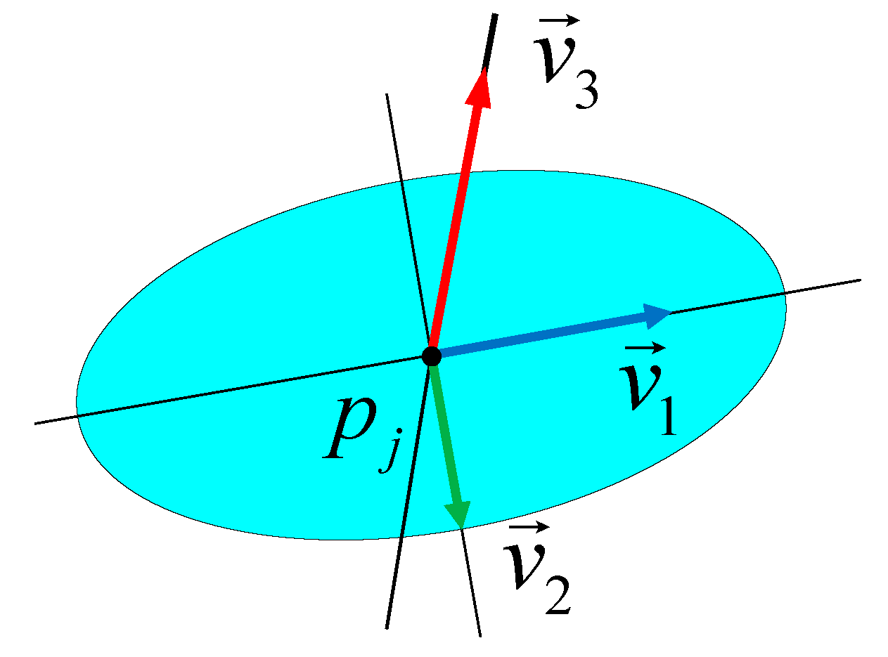
pj). then, rank the eigenvalues in descending order. The established LRF is shown in
Figure 6:
Step 5: To minimize the interference of diffusion points along the main direction on detection, non-maximum suppression (
NMS) is applied to the salient features within
r. Set threshold
ε1 and
ε2, Keypoints need to meet:
Step 6: Repeat the above steps until all points are traversed.
ISS has low sensitivity to point cloud distribution and noise type, and has good stability; The accuracy of local feature description may not be as good as FPFH, but ISS is very efficient and suitable for real-time applications.
When the PCD is large, the process of searching similar sets and screening the best transformation matrix in 4PCS is slow and time-consuming. Most of the keypoints extracted by ISS are invariant to rotation, scale, and affine transformation, and retain local geometric features, which can be used as a stable and reliable initial point set for pairing. This point set can greatly improve the accuracy of the 4PCS algorithm in solving the optimal transformation. In addition, limiting the matching points to the keypoints set can greatly reduce the amount of calculation and make the coarse registration faster.
3.2. SSM-NDT Fine Registration
The traditional NDT algorithm uses PDF to solve the maximum possibility of surface shape coincidence of all blocks. When the local shape difference is large, the effect is poor, and the surface shape similarity should be improved first, so as to reduce the probability of matching dislocation caused by surface deviation.
Figure 7.
Fuse density features to construct SSM.
Figure 7.
Fuse density features to construct SSM.
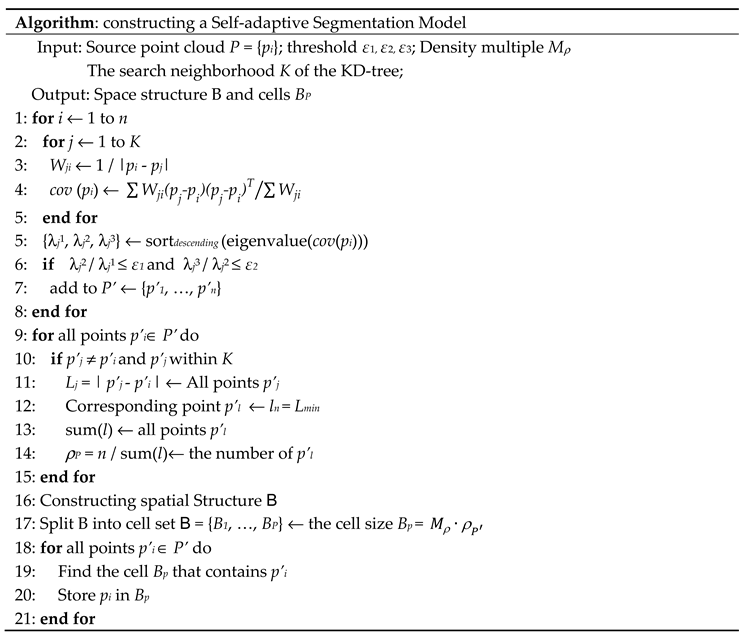
In addition, the size of the block directly affects the number of point clouds in the block, the distribution of point clouds and the total number of blocks, so setting a reasonable block size is a crucial step. To this end, a self-adaptive segmentation algorithm based on point cloud density features is proposed. Through this method, a segmentation model is constructed to cut the point cloud to cope with different distributions of PCD. The process of constructing a self-adaptive segmentation model is shown in
Figure 7.
Let the Euclidean distance between any point
pi and other points in point cloud
P be
L, and the set of all
L corresponding to
pi is
ξi = {
L1, …,
Ln-1}. If all the elements in the set a are arranged in descending order, the minimum distance value
li of
pi is:
Where: n is the number of points; q is any point that does not coincide with pi.
Determining one
L requires finding and computing
n-1
Ls, which is extremely inefficient and unnecessary. By building a KD-tree to search, the calculation range is narrowed to around
pi. At this time, the density
of point cloud
P is:
To construct SSM based on point cloud density, a parameter that can adjust the block size is introduced: density multiple
Mρ. Embed the model in equation (7) to become
FSSM:
Where: kρ is the model quantity constructed in point cloud P; Vmax is the volume of the maximum bounding box of point cloud P; Rk is the segmented point cloud block {r1, ..., rm} under the kρ model quantity, rm is a point within the block.
The pseudo program code for constructing an SSM is as follows.

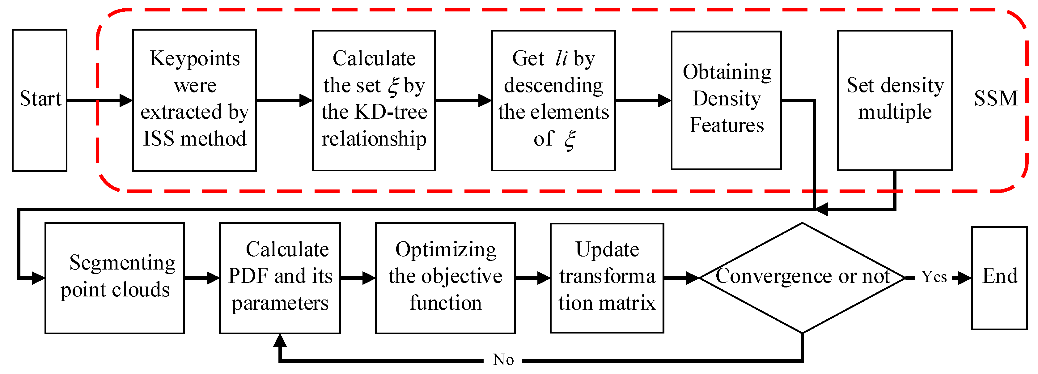
Additionally, the process of SSM-NDT is as follows:
Figure 8.
Flow chart of SSM-NDT.
Figure 8.
Flow chart of SSM-NDT.
SSM-NDT is an adaptive registration algorithm, which can produce accurate matching results in both dense and sparse regions, and has strong anti-interference. In PCD, each point is considered to carry information, and its relationship with nearby points determines whether the information is of high value. According to equation (14), the point cloud density is determined by the minimum distance li corresponding to all points. It can be inferred that there should be at least one point within the area with any point pi as the center and li as the radius. If not, it means that the surrounding of the point is relatively sparse and the information load is low; On the contrary, it is dense and has a high probability of containing high-quality information. Therefore, if you want to improve the registration accuracy, you can put more point clouds in the same block, but this will increase the calculation time.
4. Experiment and Analysis
4.1. Experimental Environment
The experimental equipment is a laptop with a processor of Intel(R)Corei5-7300HQCPU@2.50GHz, 8GRAM, and a 64-bit Windows 10 operating system, the program runs in Visual Studio 2022+PCL (Point Cloud Library)1.12.0 [
38]. The experiment verifies the effectiveness of the algorithm on the PandaSet dataset and The Real LiDAR-Derived PCD.
The comparison mainly includes registration accuracy, runtime, and anti-interference. Among them,
RMSE, Deviation (
Dev), Standard Deviation (
StDev), and
Recall were used as quantitative indicators for judging registration precision:
Where: n is the number of point-pairs; N is the number of points; xi and yi are a point-pair; is the mean of xi; TP (True Positive) is the number of correctly matched point-pairs; FN (False Negative) is the number of incorrectly matched point-pairs.
Specifically, RMSE describes the accuracy of the algorithm for real-world transformations; Dev measures the partial accuracy and stability of the algorithm; The smaller StDev, the more consistent and accurate the calculation results; Recall measures the ability of the algorithm to correctly match point-pairs.
4.2. Parameter Settings
The influence of parameter values on the method cannot be underestimated. The rules for setting parameters in ISS can be referred to reference [
24], the effects of voxel grid size
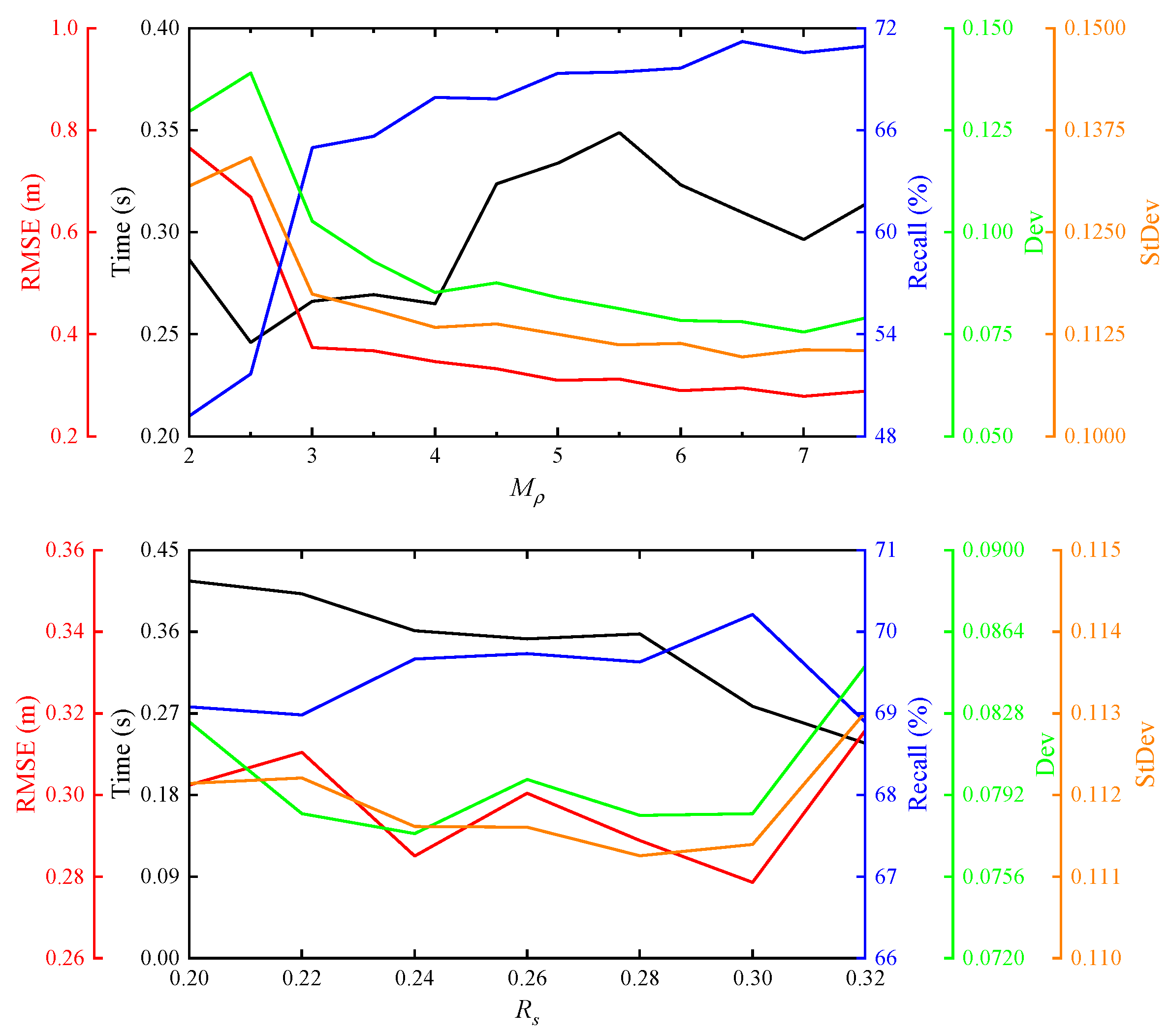
Rs and density multiple
Mρ on the performance of SSM-NDT are shown in
Figure 9.
As shown in
Figure 9, the
Mρ value is positively correlated with registration accuracy. At
Mρ = 3, RMSE, Dev, and StDev rapidly decrease around, and then remain stable; The
Mρ value and running time show a "W" shape with low left and high right. The
Rs value has a negative correlation with the running time; RMSE, Dev, and StDev show a "W" or "V" shaped trend as Rs increase, while the recall rate shows an inverted "U" shape.
FSSM varies with
Mρ and
for different PCDs. Since the change in
between two frames is small,
Mρ becomes the most important dependent variable. According to equation (15), if
Mρ decreases,
kρ increases, and
rm decreases. This means that the number of points in each block will decrease, while the total number of blocks increases. Although this can reduce the number of
, it cannot contain enough surface shape features, and the accuracy will decrease; if
Mρ is too large, the calculation amount of each
will increase, more feature information can be included, and the accuracy will increase, but the running time will increase sharply. The parameters set for the experiment are shown in
Table 1.
4.3. PandaSet Dataset
PandaSet, an open-source commercial dataset, is collected by a forward 128-line MEMS LiDAR (PandarGT) and a mechanically rotated 64-line LiDAR (Pandar64). This dataset covers the most challenging driving conditions in L5 autonomous driving, including complex urban environments, dense traffic and pedestrians, steep hills, buildings, and lighting conditions at different times.
4.3.1. Accuracy
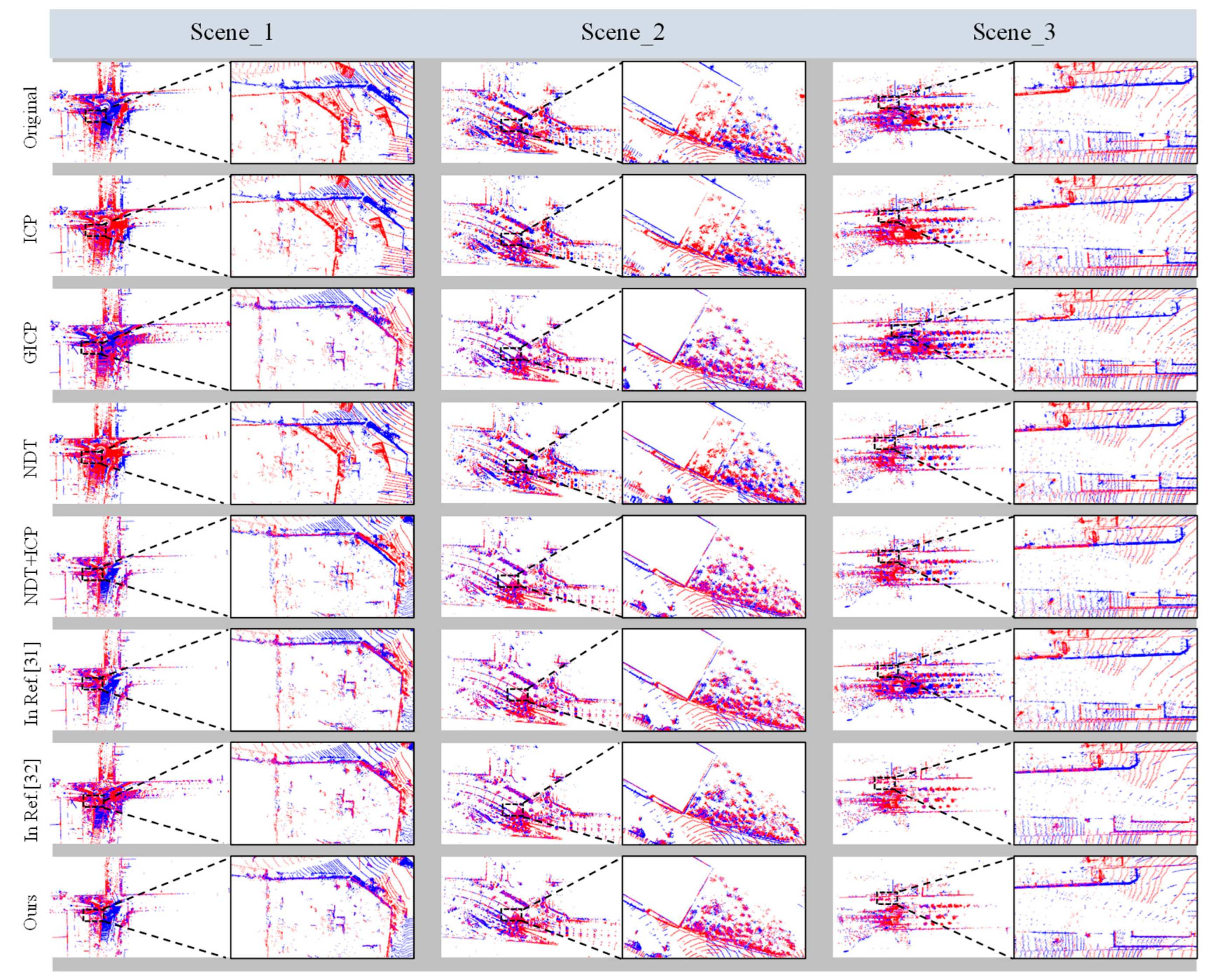
Three scenes are randomly selected and two frames are selected from each scene. Our method was compared with ICP, GICP, NDT, NDT+ICP, In Ref. [
30] algorithm, and In Ref. [
31] algorithm. The registration effects are shown in
Figure 10.
Figure 10.
Visual comparison diagram of various algorithms.
Figure 10.
Visual comparison diagram of various algorithms.
Figure 11.
Registration accuracy comparison chart.
Figure 11.
Registration accuracy comparison chart.
Different from Scene_1 and Scene_2, the shapes of buildings on both sides of the road in Scene_3 are similar, the corners of buildings are fewer, and there are many pedestrians. These characteristics mean that the surface features of the point cloud are not obvious, there are many noises, and the matching distance is large, etc., which makes the registration difficulty of Scene_3 significantly higher than others.ICP and NDT only reduce a small part of the rotation error, and the translation error is still very large. GICP, NDT+ICP, and In Ref. [
30] can only reduce the error under Scene_1 and Scene_2. Only In Ref. [
31] and Ours reduce the error in all scenes. In the enlarged figures of Scene_2 and Scene_3, it is shown that the overlap degree of In Ref. [
31] is lower than Ours.
Most of the above algorithms rely on parameter settings, and improper parameter settings may lead to the algorithm falling into local optima. For more objectivity, each method was repeated 500 times.
Figure 11 shows the comparison of the mean values of RMSE, Dev, StDev, and Recall. The indicators of Ours in the three scenes rank high, and there is a small gap with the optimal method. Especially in Scene_ 3, Ours is not only the smallest on RMSE, Dev, and STDev, and also the largest on recall.
4.3.2. Time
For practical application scenarios, the registration time between two frames is a very important indicator.
Table 2 lists the running time of each method and whether they are successfully registered (SR).
According to the data in
Table 2, ICP, 4pcs, and NDT failed all registration. ICP is sensitive to the initial position and fails when the point-to-point distance is large; 4pcs does not need iteration and its running time is very short; NDT takes abnormal time to match when the point cloud density distribution is uneven.
GICP, NDT+ICP, and In Ref. [
30] were successfully registered in Scene_1 and Scene_2. GICP constructs the cost function through the covariance matrix of the surface based on ICP, which improves the success rate but takes more time; NDT+ICP simplifies the point cloud through the voxel filter, which greatly reduces the time; the average time of the method in In Ref. [
30] is the same as that of NDT+ICP is similar, and its registration is better as shown in
Figure 9. In Scene_3, only the In Ref. [
31] and Ours are successfully registered. Ours takes at least 70%-80% less time in all scenarios than others. Therefore, the method in this paper has great advantages in efficiency, while taking into account the accuracy.
4.3.3 Stability
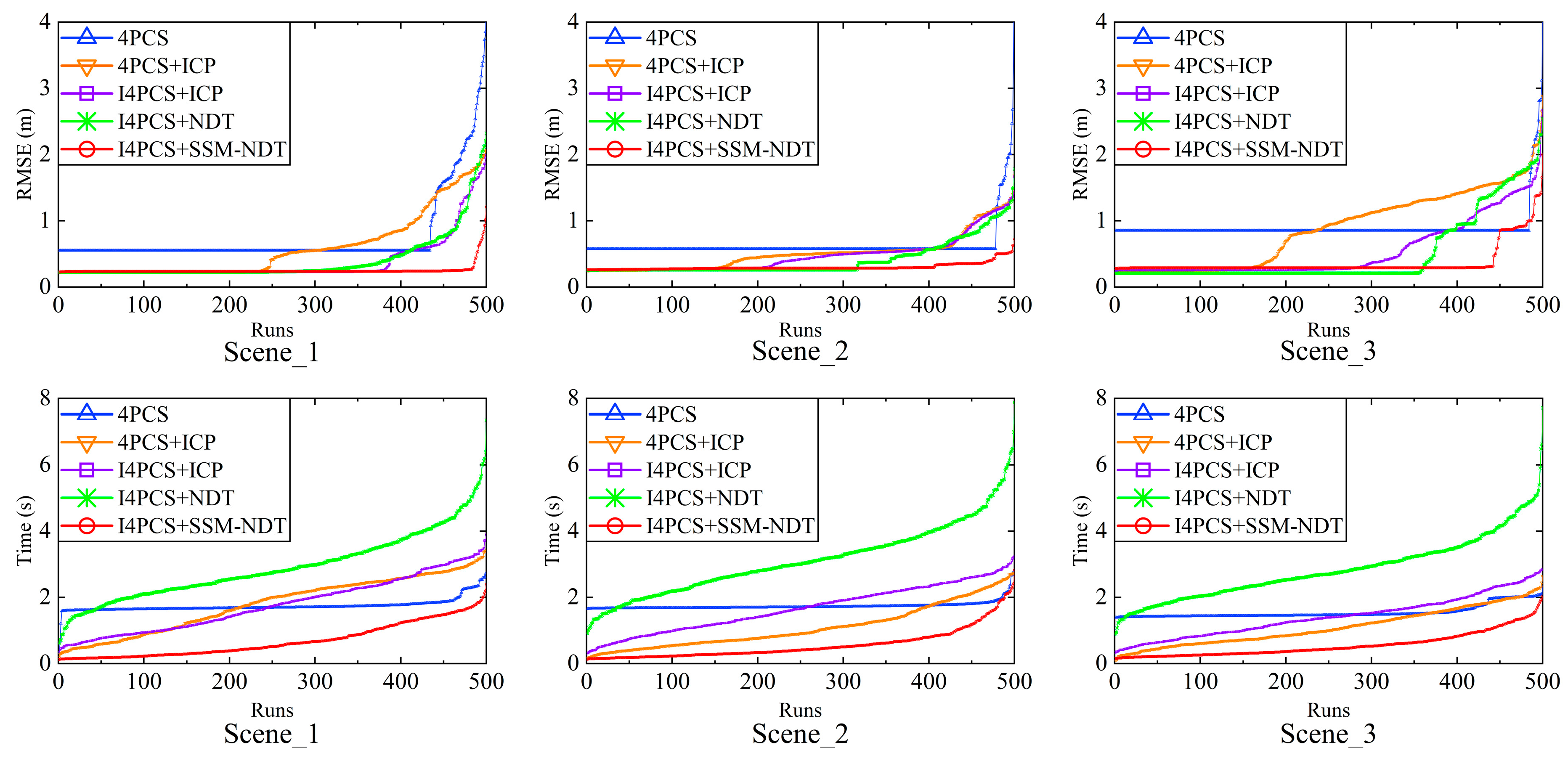
4PCS is similar to the RANSAC framework, which is uncertain, and it is necessary to improve stability. By matching different coarse and fine registrations, we had explored the influence of I4PCS and SSM-NDT on the stability respectively. The results of 500 experiments are arranged in ascending order, and the changes are shown in
Figure 12.
According to the change of the RMSE curve, I4PCS+ICP tends to the lower right corner than 4PCS+ICP, which indicates that I4PCS can effectively reduce the frequency and amplitude of anomalies than 4PCS. Similarly, the comparison between I4PCS+NDT and I4PCS+SSM-NDT shows that introducing SSM into NDT can effectively reduce instability. According to the change of the time curve, I4PCS+ICP and 4PCS+ICP approximately overlap, indicating that their efficiency is not much different; while 4PCS+KDF-NDT only slightly increases at the end, indicating that KDF-NDT takes less time and reduces fluctuations.
Figure 12.
Fluctuations in Results of Different Schemes (Arrange the results of 500 experiments in ascending order).
Figure 12.
Fluctuations in Results of Different Schemes (Arrange the results of 500 experiments in ascending order).
The analysis shows that I4PCS and SSM-NDT mainly improve accuracy and efficiency respectively, and both improve the stability together. In Scene_2 and Scene_3, although the introduction of ISS as a pre-step will increase the time-consuming of rough registration, it can reduce the calculation amount of fine registration and shorten the overall time; SSM-NDT can correct the abnormality of coarse registration in time.
3.3.4. Anti-Interference
During the outdoor scanning process of LiDAR, it is inevitable that the collected data will be interfered with. Thus, anti-interference is one of the important indicators to evaluate the quality of the method. To verify the anti-interference ability of the method, the following four types of interference (IF) are added to Scene_1:
Remove 10% of the local point cloud (IF1): there are obstructions or the light intensity is very weak.
Remove 20% of the global point cloud (IF2): under the influence of bad weather, data loss may occur.
Add 20% local noise (IF3): strong reflection may occur on the surface with large curvature.
Add 50% global noise (IF4): beams of different lidars may interfere with each other.
The PCD after interference is shown in
Figure 13, and the anti-interference ability of the method is quantitatively evaluated by the relative error (RE). The relative error distribution of each index is shown in
Figure 14.
Where: IFBefore and IFAfter are the values before and after the interference respectively.
The relative accuracy error of most algorithms is smaller in IF2 and IF4 than in IF1 and IF3, and the time error is smaller in IF3 and IF4. In terms of accuracy, the error of the method in this paper is small among the four types of disturbances; in terms of time, the data in
Table 2 shows that the algorithm in this paper takes a very short time, although the error performance is average, and the absolute value of the error is less than 0.2s.
Figure 13.
The image after adding four kinds of interference to Scene_1 (purple is the origin cloud; green is the Gaussian noise added).
Figure 13.
The image after adding four kinds of interference to Scene_1 (purple is the origin cloud; green is the Gaussian noise added).
Figure 14.
Scatter plot of relative error of each algorithm before and after four types of interference.
Figure 14.
Scatter plot of relative error of each algorithm before and after four types of interference.
Different methods exhibit different immunity to different disturbances. Ours can be anti-interference in the coarse and fine registration. ISS is more inclined to areas with high curvature and high features, while noise is usually not in this area; SSM incorporates a large number of surface features to reduce the influence of local area anomalies.
4.4. The Real LiDAR-Derived PCD
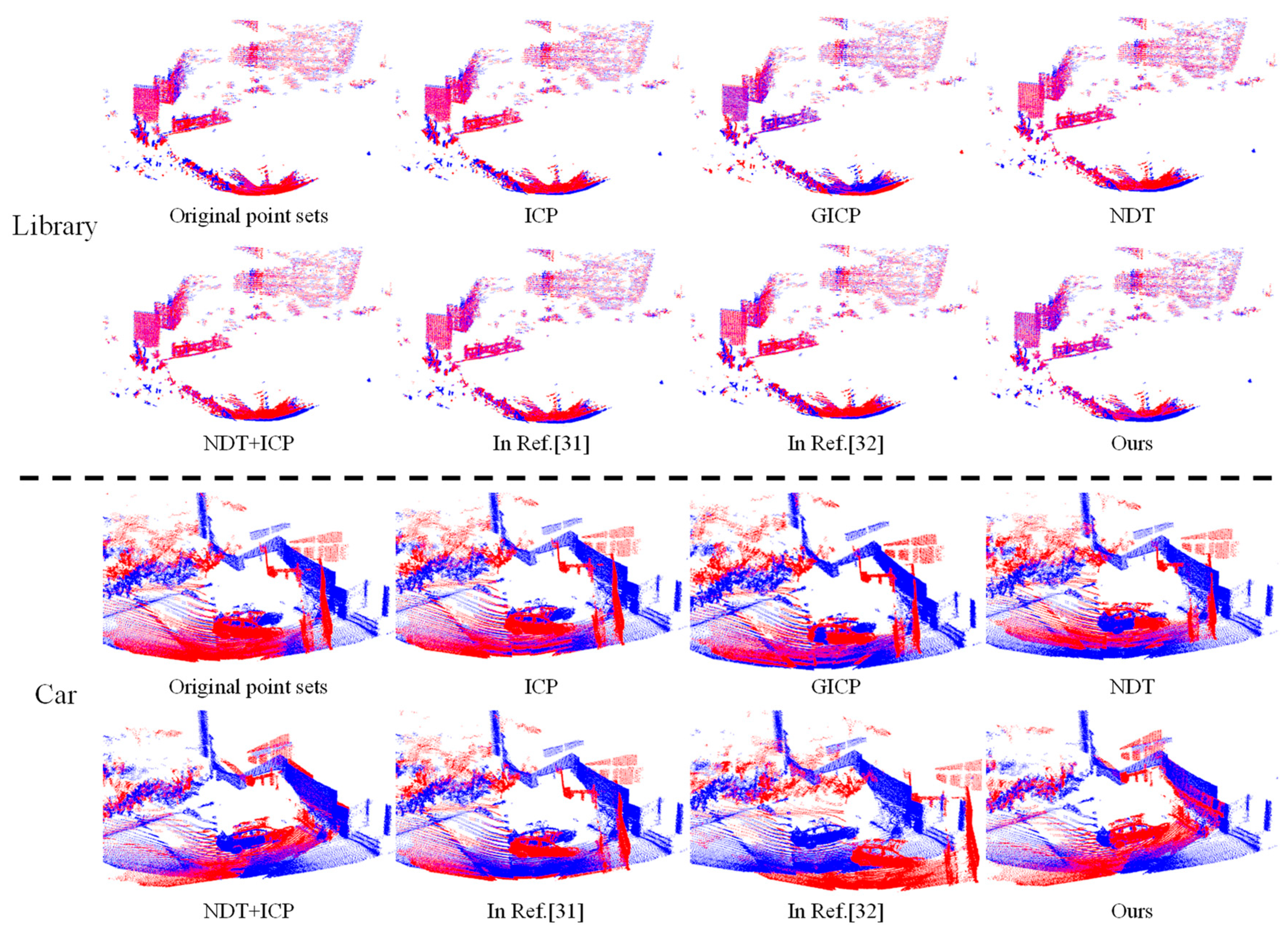
To further verify the effectiveness and applicability, we had tested the real PCD collected by forward MEMS LiDAR (RS-LiDAR M1, RoboSense, Shenzhen, China). The PCD perspective is relatively small and there are few matching targets.
Figure 14 and
Table 3 show the registration results on this PCD.
In the Library scene, the offset between two frames is small, and most of the methods can be registered successfully. The Mean Time of Ours is only 0.32s, which is at least 60% higher than other methods. The rotation offset between two frames in the Car scene is large, and only NDT+ICP and Ours are successful. The accuracy of Ours is higher, and the time is only 0.84s, which is 65.5% higher than that of NDT+ICP. Therefore, the algorithm in this paper has great advantages in similar scenarios.
Internal factors that affect time include algorithm principles and initial values; external factors are related to PCD. The algorithm in this paper is efficient and concise. Firstly, the improved voxel filtering simplifies PCD; secondly, I4PCS does not need iteration and is highly efficient; finally, SSM-NDT automatically determines the optimal segmentation size to further improve efficiency. Therefore, in each experimental scenario, the mean time consumption of this algorithm is significantly less than that of others, and the efficiency is far ahead.
Figure 15.
Registration results of The Real LiDAR-Derived PCD.
Figure 15.
Registration results of The Real LiDAR-Derived PCD.
Table 3.
Comparison of evaluation indicators for registration results of The Real LiDAR-Derived PCD.
Table 3.
Comparison of evaluation indicators for registration results of The Real LiDAR-Derived PCD.
| Algorithm |
Mean RMSE |
Mean Dev |
Mean StDev |
Mean Recall |
Mean Time |
Max Time |
SR |
| Library(N=50215) |
|
|
|
|
|
|
| ICP |
0.2240 |
0.1136 |
0.1391 |
67.4818 |
4.3752 |
5.1180 |
✓ |
| GICP |
0.1672 |
0.0717 |
0.1118 |
65.8270 |
2.1092 |
5.201 |
✓ |
| 4PCS |
0.4744 |
0.0896 |
0.1137 |
56.2409 |
1.5248 |
2.5150 |
|
| NDT |
0.1707 |
0.0711 |
0.1116 |
64.6528 |
8.0606 |
9.7360 |
✓ |
| NDT+ICP |
0.1690 |
0.0722 |
0.1131 |
66.6853 |
3.2195 |
3.5250 |
✓ |
| In Ref. [30] |
0.1677 |
0.0738 |
0.1116 |
64.9547 |
1.5812 |
1.8710 |
✓ |
| In Ref. [31] |
0.2008 |
0.0895 |
0.1139 |
66.9021 |
0.8389 |
1.4030 |
✓ |
| Ours |
0.1736 |
0.0731 |
0.1135 |
65.4235 |
0.3276 |
3.5640 |
✓ |
| Car(N=72770) |
|
|
|
|
|
|
| ICP |
0.1351 |
0.0858 |
0.1268 |
64.9637 |
1.2060 |
1.3260 |
|
| GICP |
0.1290 |
0.0773 |
0.11644 |
64.2627 |
1.6893 |
2.149 |
|
| 4PCS |
0.1771 |
0.0932 |
0.1267 |
63.3158 |
2.6987 |
6.0140 |
|
| NDT |
0.1311 |
0.1122 |
0.1357 |
56.5143 |
12.7207 |
13.8180 |
|
| NDT+ICP |
0.1268 |
0.0741 |
0.1051 |
76.9665 |
2.4270 |
2.9370 |
✓ |
| In Ref. [30] |
0.2071 |
0.0910 |
0.1165 |
66.2869 |
1.4699 |
3.1430 |
|
| In Ref. [31] |
0.4013 |
0.1455 |
0.1347 |
44.4968 |
1.3607 |
2.0880 |
|
| Ours |
0.1244 |
0.0546 |
0.0962 |
72.2800 |
0.8414 |
5.1380 |
✓ |
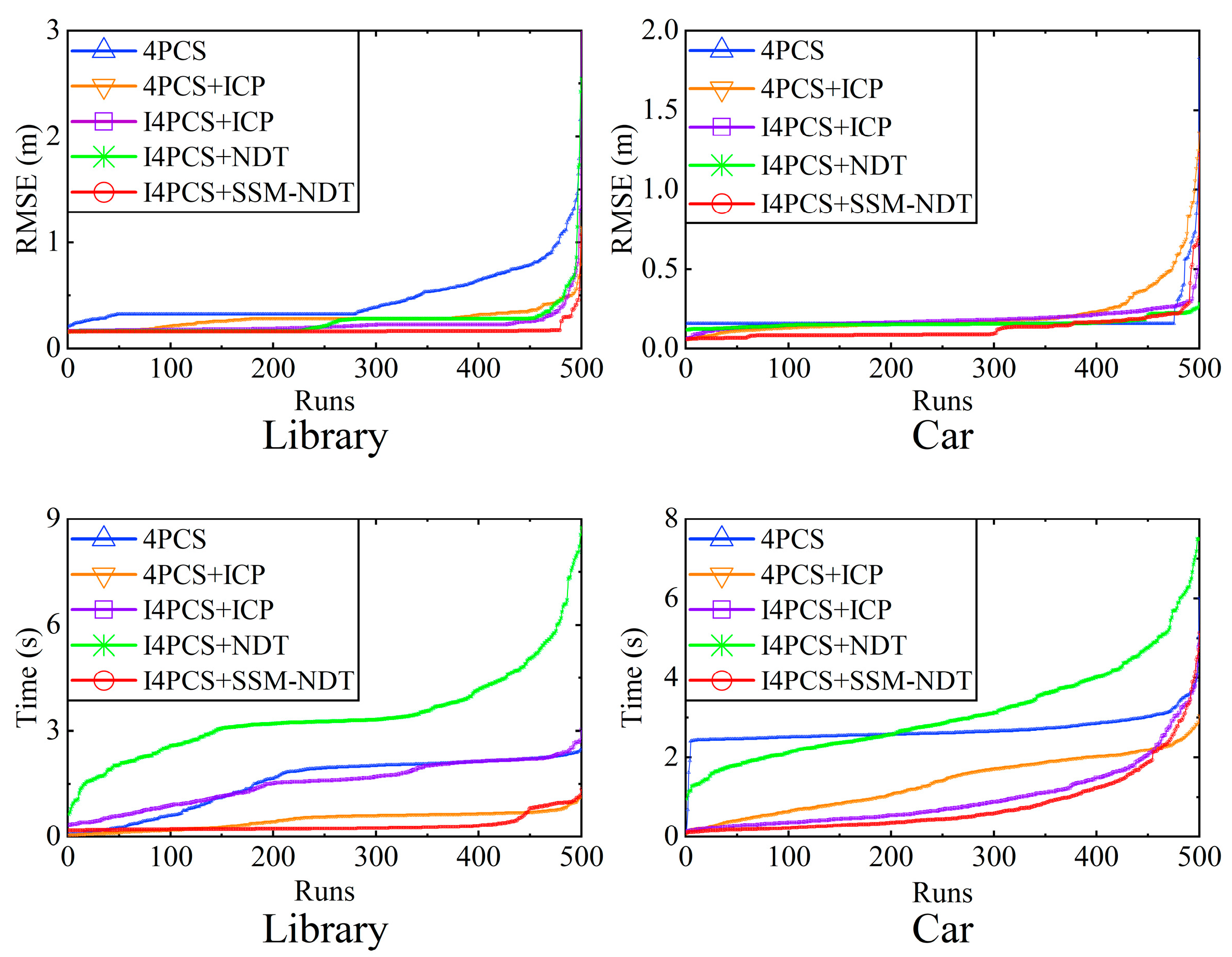
Figure 16.
Registration changes of The Real LiDAR-Derived PCD.
Figure 16.
Registration changes of The Real LiDAR-Derived PCD.
In the car scene stability test results, unexpectedly, the change of the end segment of the I4PCS+SSM-NDT curve is roughly the same as that of other algorithms, indicating that the possibility of errors has not been reduced. It is speculated that the continuity between the two frames of the scene is insufficient and the overlap is too small.
5. Conclusion and Outlook
A fast registration method based on MEMS lidar target point cloud is proposed. The method uses a pass-through filter and voxel filter with minimum points number to preprocess; Using the keypoints of ISS as two input point clouds, 4PCS effectively obtains the initial transformation matrix; In the precise registration process, the density feature information of keypoints is used to create the SSM to retrofit the NDT. This method is called SSM-NDT. Considering the distribution characteristics of different point clouds, SSM-NDT solves the problems of poor applicability and low efficiency of traditional NDT algorithm.
Experiments were carried out in PandaSet and The Real LiDAR-Derived PCD, the results show that when the registration accuracy is similar, the registration time is significantly reduced compared with other methods, and the improvement is more than 60%. In addition, it also shows anti-interference in a variety of abnormal conditions.
One limitation of the proposed algorithm is that if the scene continuity is very low, the probability of abnormal registration cannot be reduced. To overcome this limitation, in future research, we plan to consider the surface smoothness and connectivity of point clouds in the registration process to optimize the accuracy of fast alignment when the overlap is low.
Author Contributions
Conceptualization, B.L. and X.L; methodology, B.L; project administration, X.L.; software, B.L.; validation, B.L. and M.L.; resources, C.L.; datacuration, B.L.; writing—original draft preparation, B.L. and S.L; writing—review and editing, B.L., X.L. and S.L.; visualization, B.L.; supervision, X.L. and M.L.; funding acquisition, X.L. All authors have read and agreed to the published version of the manuscript.
Funding
This paper is partly supported by the Natural Science Foundation of Jilin Province under grant YDZJ202201ZYTS655.
Data Availability Statement
Acknowledgments
The authors thank the Mechanical and Control Engineering 219 Lab of Baicheng Normal University.
Conflicts of Interest
The authors declare no conflict of interest.
References
- Shao, H.; Zhang, Z.; Feng, X.; Zeng, D. SCRnet: A Spatial Consistency Guided Network Using Contrastive Learning for Point Cloud Registration. Symmetry 2022, 14, 140. [Google Scholar] [CrossRef]
- Li, X.; Mo, S.; Huang, H.; Yang, S. Multi-source point cloud registration method based on automatically calculating overlap. Infrared and Laser Engineering 2021, 50, 270–278. [Google Scholar] [CrossRef]
- Besl, P.J.; McKay, N.D. A method for registration of 3-D shapes. IEEE Transactions on Pattern Analysis and Machine Intelligence 1992, 14, 239–256. [Google Scholar] [CrossRef]
- Chen, Y.; Medioni, G. Object modeling by registration of multiple range images. In Proceedings of the Proceedings. 1991 IEEE International Conference on Robotics and Automation, 9-11 April 1991, 1991; pp. 2724-2729 vol.2723. [CrossRef]
- Segal, A.; Hähnel, D.; Thrun, S. Generalized-ICP; 2009. [CrossRef]
- Chetverikov, D.; Stepanov, D.; Krsek, P. Robust Euclidean alignment of 3D point sets: the trimmed iterative closest point algorithm. Image Vis. Comput. 2005, 23, 299–309. [Google Scholar] [CrossRef]
- Serafin, J.; Grisetti, G. NICP: Dense normal based point cloud registration. In Proceedings of the 2015 IEEE/RSJ International Conference on Intelligent Robots and Systems (IROS), 28 Sept.-2 Oct. 2015, 2015; pp. 742-749. [CrossRef]
- Bae, K.-H.; Lichti, D.D. A method for automated registration of unorganised point clouds. ISPRS J. Photogramm. Remote. Sens. 2008, 63, 36–54. [Google Scholar] [CrossRef]
- Wang, X.; Li, Y.; Peng, Y.; Ying, S. A Coarse-to-Fine Generalized-ICP Algorithm With Trimmed Strategy. IEEE Access 2020, 8, 40692–40703. [Google Scholar] [CrossRef]
- Zhang, J.; Yao, Y.; Deng, B. Fast and Robust Iterative Closest Point. IEEE Trans Pattern Anal Mach Intell 2022, 44, 3450–3466. [Google Scholar] [CrossRef]
- Magnusson, M.; Lilienthal, A.; Duckett, T. Scan registration for autonomous mining vehicles using 3D-NDT. J. Field Robot. 2007, 24, 803–827. [Google Scholar] [CrossRef]
- Aiger, D.; Mitra, N.J.; Cohen-Or, D. 4-points congruent sets for robust pairwise surface registration. ACM Trans. Graph. 2008, 27, 1–10. [Google Scholar] [CrossRef]
- Theiler, P.W.; Wegner, J.D.; Schindler, K. Keypoint-based 4-Points Congruent Sets – Automated marker-less registration of laser scans. ISPRS J. Photogramm. Remote. Sens. 2014, 96, 149–163. [Google Scholar] [CrossRef]
- Sipiran, I.; Bustos, B. A Robust 3D Interest Points Detector Based on Harris Operator; 2010; pp. 7–14. [Google Scholar] [CrossRef]
- Lowe, D.G. Object recognition from local scale-invariant features. In Proceedings of the Proceedings of the Seventh IEEE International Conference on Computer Vision, 20-27 Sept. 1999, 1999; pp. 1150-1157 vol.1152. [CrossRef]
- Xu, Y.; Boerner, R.; Yao, W.; Hoegner, L.; Stilla, U. Pairwise coarse registration of point clouds in urban scenes using voxel-based 4-planes congruent sets. ISPRS J. Photogramm. Remote. Sens. 2019, 151, 106–123. [Google Scholar] [CrossRef]
- Rusu, R.B.; Blodow, N.; Marton, Z.C.; Beetz, M. Aligning point cloud views using persistent feature histograms. In Proceedings of the 2008 IEEE/RSJ International Conference on Intelligent Robots and Systems, 22-26 Sept. 2008, 2008; pp. 3384-3391. [CrossRef]
- Rusu, R.B.; Blodow, N.; Beetz, M. Fast Point Feature Histograms (FPFH) for 3D registration. In Proceedings of the 2009 IEEE International Conference on Robotics and Automation, 12-17 May 2009, 2009; pp. 3212-3217. [CrossRef]
- Salti, S.; Tombari, F.; Di Stefano, L. SHOT: Unique signatures of histograms for surface and texture description. Comput. Vis. Image Underst. 2014, 125, 251–264. [Google Scholar] [CrossRef]
- Frome, A.; Huber, D.; Kolluri, R.; Bülow, T.; Malik, J. Recognizing Objects in Range Data Using Regional Point Descriptors. In Proceedings of the Computer Vision - ECCV 2004, Berlin, Heidelberg, 2004//, 2004; pp. 224-237. [CrossRef]
- Li, M.; Hashimoto, K. Curve Set Feature-Based Robust and Fast Pose Estimation Algorithm. Sensors 2017, 17, 1782. [Google Scholar] [CrossRef]
- Tao, W.; Hua, X.; Chen, Z.; Tian, P. Fast and Automatic Registration of Terrestrial Point Clouds Using 2D Line Features. Remote. Sens. 2020, 12, 1283. [Google Scholar] [CrossRef]
- Yue, X.; Liu, Z.; Zhu, J.; Gao, X.; Yang, B.; Tian, Y. Coarse-fine point cloud registration based on local point-pair features and the iterative closest point algorithm. Appl. Intell. 2022, 52, 12569–12583. [Google Scholar] [CrossRef]
- Zhang, X.; Gao, R.; Sun, Q.; Cheng, J. An Automated Rectification Method for Unmanned Aerial Vehicle LiDAR Point Cloud Data Based on Laser Intensity. Remote. Sens. 2019, 11, 811. [Google Scholar] [CrossRef]
- Prokop, M.; Shaikh, S.A.; Kim, K.-S. Low Overlapping Point Cloud Registration Using Line Features Detection. Remote Sens. 2020, 12, 61. [Google Scholar] [CrossRef]
- Chen, S.; Nan, L.; Xia, R.; Zhao, J.; Wonka, P. PLADE: A Plane-Based Descriptor for Point Cloud Registration With Small Overlap. IEEE Trans. Geosci. Remote. Sens. 2019, 58, 2530–2540. [Google Scholar] [CrossRef]
- Wang, J.; Wang, P.; Li, B.; Fu, R.; Zhao, S.; Zhang, H. Discriminative optimization algorithm with global–local feature for LIDAR point cloud registration. Int. J. Remote. Sens. 2021, 42, 9003–9023. [Google Scholar] [CrossRef]
- Yang, J.; Luo, W.; Zhang, Y.; Chang, B.; Zheng, R.; Wu, M. Establishment of a Coal Mine Roadway Model Based on Point Cloud Feature Matching. Math. Probl. Eng. 2022, 2022, 1–14. [Google Scholar] [CrossRef]
- Yang, J.; Wang, C.; Luo, W.; Zhang, Y.; Chang, B.; Wu, M. Research on Point Cloud Registering Method of Tunneling Roadway Based on 3D NDT-ICP Algorithm. Sensors 2021, 21, 4448. [Google Scholar] [CrossRef] [PubMed]
- Xu, G.; Pang, Y.; Bai, Z.; Wang, Y.; Lu, Z. A Fast Point Clouds Registration Algorithm for Laser Scanners. Appl. Sci. 2021, 11, 3426. [Google Scholar] [CrossRef]
- Baek, J.; Park, J.; Cho, S.; Lee, C. 3D Global Localization in the Underground Mine Environment Using Mobile LiDAR Mapping and Point Cloud Registration. Sensors 2022, 22, 2873. [Google Scholar] [CrossRef]
- Wu, B.; Yang, L.; Wu, Q.; Zhao, Y.; Pan, Z.; Xiao, T.; Zhang, J.; Wu, J.; Yu, B. A Stepwise Minimum Spanning Tree Matching Method for Registering Vehicle-Borne and Backpack LiDAR Point Clouds. IEEE Trans. Geosci. Remote. Sens. 2022, 60, 1–13. [Google Scholar] [CrossRef]
- Wang, H.; Liang, H.; Li, Z.; Zhou, P.; Chen, L. A fast coarse-to-fine point cloud registration based on optical flow for autonomous vehicles. Appl. Intell. 2023, 1–18. [Google Scholar] [CrossRef]
- Li, J.; Zhan, J.; Zhou, T.; Bento, V.A.; Wang, Q. Point cloud registration and localization based on voxel plane features. ISPRS J. Photogramm. Remote. Sens. 2022, 188, 363–379. [Google Scholar] [CrossRef]
- Theodose, R.; Denis, D.; Chateau, T.; Fremont, V.; Checchin, P. A Deep Learning Approach for LiDAR Resolution-Agnostic Object Detection. IEEE Trans. Intell. Transp. Syst. 2021, 23, 14582–14593. [Google Scholar] [CrossRef]
- Biber, P.; Strasser, W. The normal distributions transform: a new approach to laser scan matching. In Proceedings of the Proceedings 2003 IEEE/RSJ International Conference on Intelligent Robots and Systems (IROS 2003) (Cat. No.03CH37453), 27-31 Oct. 2003, 2003; pp. 2743-2748 vol.2743. [CrossRef]
- Zhong, Y. Intrinsic shape signatures: A shape descriptor for 3D object recognition. In Proceedings of the 2009 IEEE 12th International Conference on Computer Vision Workshops, ICCV Workshops, 2009; pp. 689-696. [CrossRef]
- Munaro, M.; Rusu, R.B.; Menegatti, E. 3D robot perception with Point Cloud Library. Robot. Auton. Syst. 2016, 78, 97–99. [Google Scholar] [CrossRef]
|
Disclaimer/Publisher’s Note: The statements, opinions and data contained in all publications are solely those of the individual author(s) and contributor(s) and not of MDPI and/or the editor(s). MDPI and/or the editor(s) disclaim responsibility for any injury to people or property resulting from any ideas, methods, instructions or products referred to in the content. |
© 2023 by the authors. Licensee MDPI, Basel, Switzerland. This article is an open access article distributed under the terms and conditions of the Creative Commons Attribution (CC BY) license (http://creativecommons.org/licenses/by/4.0/).

