
Submitted:
19 June 2023
Posted:
20 June 2023
You are already at the latest version
Abstract
We study two fundamental linguistic channels ‒ the Sentences and the Interpunctions channels ‒ and show they can reveal deeper connections between texts. The theory applied does not follow the actual paradigm of linguistic studies. As study‒case, we consider the Greek New Testament, with the purpose of determining mathematical connections between its texts and possible differences in writing style (mathematically defined) of writers, and in reading skill required to their readers. The analysis is based on deep‒language parameters and communication/information theory. To set the New Testament texts in the larger Greek Classical Literature, we consider texts written by Aesop, Polybius, Flavius Josephus and Plutarch. The results largely confirm what scholars have found about the New Testament texts giving, therefore, credibility to the theory. The gospel according to John is very similar to Fables written by Aesop. Surprisingly, the Epistle to the Hebrews and Apocalypse, are each other “photocopy” in the two linguistic channels, and not linked to all other texts. These two texts deserve further study by historians of the early Christian Church Literature at the level of meaning, readers and possible Old Testament texts which might have influenced them. The theory can guide scholars to study any literary corpus.
Keywords:
Apocalypse
; Deep‒language
; Greek New Testament
; Greek Classical Literature
; Epistle to the Hebres
; Interpunctions
; Likeness index
; Linguistic channels
; Sentences
; Signal‒to‒noise ratio
; Vectors
1. A mathematical theory of texts outside the paradigm of natural language processing
In recent papers [1,2,3,4,5,6,7,8], we have developed a general theory on the deep‒language mathematical structure of literary texts (or any long text), including their translation. The theory is based on linguistic communication channels ‒ suitable defined‒ always contained in texts and based on the theory of regression lines [9,10] and Shannon’s communication and information theory [11].
In our theory, “translation” means not only the conversion of a text from a language to another language – what is properly understood as translation – but also how some linguistic parameters of a text are related to those of another text, either in the same language or in another language. “Translation”, therefore, refers also to the case a text is mathematically compared (metaphorically “translated”) to another text, whichever is the language of the two texts [2].
The theory does not follow the actual paradigm of linguistic studies. Most studies on the relationships between texts concern translation because of the importance of automatic translation. References [12‒18] report results not based on mathematical analysis of texts - as our theory does - and when a mathematical approach is used, as in References [19,20,21,22,23,24,25,26,27,28,29,30,31,32,33,34,35,36,37,38,39,40,41,42,43,44,45,46,47,48,49,50,51], most of these studies neither consider Shannon’s communication theory, nor the fundamental connection that some linguistic variables seem to have with reading ability and STM capacity [1,2,3,4,5,6,7,8]. In fact, these studies are mainly concerned with automatic translations, not with a high–level direct response of human readers, as our theory does. Very often they refer only to one very limited linguistic variable, not to sentences which convey a completely developed thought – not to deep–language parameters, as our theory does.
The theory allows to perform experiments with ancient readers − otherwise impossible – or with modern readers, by studying the literary texts of their epoch. These “experiments” can reveal unexpected similarity and dependence between texts, because they consider mathematical parameters not consciously controlled by writers, either ancient or modern, as we will also show in the present paper.
Besides the total number of characters, words, sentences and interpunctions (punctuation marks) of a text, the linguistic parameters considered in our theory are: number of words per chapter; number of sentences per chapter; number of interpunctions per chapter . Instead of referring to chapters, the analysis can refer to any chosen subdivision of a literary text, large enough to provide reliable statistics, such as few hundreds words [1,2,3,4,5,6,7,8].
We also consider four important deep–language parameters, calculated in each chapter (or in any large‒enough block text): characters per word ; words per sentence ; words per interpunctions ; interpunctions per sentence (this variable gives the number of contained in a sentence).
The parameter , also referred to as the “words interval” (i.e. an “interval” measured in words [1]) is very likely linked to readers’ STM capacity [52] and it can be used to study how much two populations of readers of diverse languages overlap in reading a literary text in translation [7].
To study the chaotic data that emerge in any language, the theory compares a text (the reference, or input text) to another text (output text, “cross‒channel”) or to itself (“self‒channel”), with a complex communication channel ‒ made of several parallel single channels [4], two of which are explicitly considered in the present paper ‒ in which both input and output are affected by “noise”, i.e. by diverse scattering of the data around a mean linear relationship, namely a regression line.
In [3] we have shown how much the mathematical structure of a literary text is saved or lost in translation. To make objective comparisons, we have defined a likeness index , based on probability and communication theory of noisy digital channels. We have shown that two linguistic parameters can be related by regression lines. This is a general feature of texts. If we consider the regression line linking (dependent variable) to (independent variable) in a reference text and the regression line linking the same parameters in another text, then of the first text can be linked to of the second text with another regression line without explicitly calculating its parameters (slope and correlation coefficient) from the samples, because the mathematical problem has the same structure of the theory developed in Reference [2].
In Reference [4] we have applied the theory of linguistic channels to show how an author shapes a character speaking to diverse audiences by diversifying and adjusting (“fine tuning”) two important linguistic communication channels, namely the Sentences channel (S‒channel) and the Interpunctions channel (I‒channel). The S‒channel links of the output text to of the input text, for the same number of words. The I‒channel links (i.e., the words intervals ) of the output text to of the input text, for the the same number of sentences.
In Reference [5] we have further developed the theory of linguistic channels by applying it to Charles Dickens’ novels and to other novels of the English Literature and found, for example, that this author was very likely affected by King James’ New Testament.
In Reference [6] we have defined a universal readability index, applicable to any alphabetical language, by including readers’ STM capacity, modelled by ; in Reference [7] we have studied the STM capacity across time and language and in Reference [8] the readability of a text across time and language.
In this paper, as the title claims, we further study linguistic communication channels ‒ namely S‒channels and I‒channels ‒ and show that they can reveal deeper connections between texts. As study‒case, we consider an important historical literary corpus, the Greek New Testament (NT), with the purpose of determining mathematical connections between its books (in the following referred to as “texts”), and possible differences in writing style (mathematically defined) of writers and in reading skill required to their readers. To set the NT texts in the Greek Classical Literature, we have considered texts written by Aesop, Polybius, Flavius Josephus and Plutarch.
The analysis is based on the deep‒language parameters and communication channels mentioned above, not explicitly known to the ancient writer/reader or, as well, to any modern writer/reader not acquainted with this theory.
After this introductory section, Section 2 recalls and defines the deep‒language parameters of texts; Section 3 recalls the vector representation of texts; Section 4 summarizes the theory of linguistic communication channels; Section 5 defines the theoretical signal–to–noise ratio in linguistic channels (S‒channels and I‒channels); Section 6 defines the experimental signal–to–noise ratio in these channels; Section 7 recalls the likeness index of texts and defines the channels quadrants; Section 8 presents an extreme synthesis of the main findings and Section 9 concludes and suggests future work. Appendix A and Appendix B reports numerical tables.
2. Deep‒language parameters of texts
The original NT Greek texts were first processed manually to delete all notes, titles and other textual material added by modern editors, therefore leaving in the end only the original texts, as it was done in Reference [53].
Interpunctions were introduced by ancient readers acting as “editors” [54]. They were well‒educated readers of the early Christian Church, very respectful of the original text and its meaning, therefore they likely maintained a correct subdivision in sentences and words intervals within sentences, for not distorting the correct meaning and emphasis of the text. In other terms, we can reasonably assume that interpunctions were effectively introduced by the author.
In Reference [53], we have compared the gospels according to Matthew (Mt), Mark (Mk), Luke (Lk), John (Jh) and the book of Acts (Ac) by considering only deep‒language parameters, not S‒channels and I‒channels, as we do in this paper. Moreover, we have presently enlarged our study‒case by including the Epistle to the Hebrews (Hb) and Apocalypse (Ap, known also as Revelation) ‒ texts which show unexpected connections – and some texts written by the historians Polybius (Po), Plutarch (Pl), Flavius Josephus (Fl) and by the story‒teller Aesop (Ae) to set the NT in the larger classical Greek Literature.
The samples used in the statistical analysis refer to chapters: for example, Matthew has 28 chapters, therefore this text is described by 28 samples for each deep‒language parameter. The list of names (“genealogy” of Jesus of Nazareth) in Matthew and in Luke have been deleted for not biasing the statistical results. Like in References [1,2,3,4,5,6,7,8,13], samples were statistically weighted with the fraction of total words, therefore in Matthew – which contains total words ‒ Chapter 5, for example, has words, therefore its weight is , not . This choice is mandatory to avoid that a short chapter (or, in general, a short text) affects the statistical results like a long one.
After this processing we have obtained the mean values of , , , reported in Table 1, and the universal readability , defined and discussed in Reference [6], here calculated with the mean values and from:
In Equation (1) we set , the mean value found in the Italian Literature, since Italian is the reference language in the definition of [1].
To set the NT texts in the Greek Classical Literature, we have considered texts written by Aesop, Polybius, Flavius Josephus and Plutarch. The rational for selecting these authors is the following: Aesop wrote texts (Fables) which may recall the parables of the gospels for their brevity and similar narrative style; Polybius, Flavius Josephus and Plutarch were historians, therefore wrote essays narrating facts, like the gospels, partially, and especially Acts. Table 2 lists texts and mean values of the deep‒language parameters of these authors. These texts have been processed manually like the NT.
The mean values of Table 1 and Table 2 can be used for a first assessment of how “close”, or mathematically similar, texts are in a Cartesian plane, by defining a linear combination of deep‒language parameters. Texts are then modelled as vectors, representation discussed in detail in [1,2,3,4,5,6] and briefly recalled in the next section.
3. Vector representation of texts
Let us consider the following six vectors of the indicated components of deep‒language parameter), ), ), ), ), ) and their resulting sum:
By considering the coordinates and of Equation (2), we obtain the scatterplot of their ending points shown in Figure 1 where the coordinates and are normalized so that Aesop’s Fables (Ae) is at the origin and Flavius Josephus’ The Jewish War (Fl) is at .
In this Cartesian plane two texts are likely connected ‒ they show close ending points ‒ if their relative Pythagorean distance is small, and are likely not connected if their distance is large. In other words, a small distance means that texts share a similar mathematical structure. This is a necessary, but not sufficient, condition for two texts being each other very likely connected.
In Figure 1, the three synoptic gospels (Mt, Mk, Lk) are the closest texts of the NT. In particular, Mt and Lk are practically coincident, almost a mathematical “photocopy” of each other, as it was also shown, with diverse analysis, in Reference [1,2]. Notice also that (Table 1) is very similar for the Synoptics but not for the other NT texts (except Hebrews), and that John (Jh) is the most readable text.
Acts and Luke, although written by the same author – as widely accepted by scholars in References [55,60], a very small selection of the huge literature on this topic ‒ are quite diverse because when Luke writes the gospel he has significant constraints because his sources are very likely shared with Matthew. But when Luke writes Acts, he has few or no sources to share with Matthew, therefore he is free to use his personal writing style oriented to narrating the early facts of the Church. It is not surprising, therefore, that Acts, because of its contents, is closer to Plutarch and Polybius than to the synpotics and that its is close to Plutarchs’ Parallel Lives (Table 1 and Table 2), therefore shading some light on the similar readability skill required to the readers of these historical narrations, and the gospels for which ranges form to .
John is distinctly diverse of Matthew, Luke and Mark, but it is very close to Aesop’s Fables.
Unexpected is the vicinity of Hebrews and Apocalyse ‒ two NT texts scholars rarely consider to be connected [60,61,62,63] – and their great distance from the gospels. Their universal readability indices are also very similar, for Hebrews and for Apocalypse.
As for the Greek historians, we can notice that they are distinctly grouped and distant from the gospels.
In conclusion, the vector modelling of texts can reveal first connections, otherwise hidden. These connections can be further addressed by studying their S‒channels and I‒channels, and the likeness index . Therefore, in the next section we first recall the theory of linguistic communication channels.
4. Theory of linguistic communication channels
In a text an independent (reference) variable (e.g. in S‒channels) and a dependent variable (e.g., can be related by a regression line (slope ) passing through the origin of the Cartesian coordinates:
Let us consider two diverse texts and . For both we can write Equation (3) for the same couple of parameters, however, in both cases Equation (3) does not give the full relationship of two parameters because it links only mean conditional values. We can write more general linear relationships which take care of the scattering of the data – measured by the correlation coefficients and , respectively, not considered in Equation (3) – around the regression lines (slopes and ):
While Equation (3) connects the dependent variable to the independent variable only on the average, Equation (4) introduces additive “noise” and , with zero mean value [2,3,4]. The noise is due to the correlation coefficient , not considered by Equation (1).
We can compare two texts by eliminating . In other words, we compare the output variable for the same value of the input variable in the two texts. In the example just mentioned, we can compare the number of sentences in two texts ‒ for an equal number of words ‒ by considering not only the mean relationship, Equation (3), but also the scattering of the data, Equation (4).
As recalled before, we refer to this communication channel as the “sentences channel” and to this processing as “fine tuning” because it deepens the analysis of the data and provides more insight into the relationship between two texts. The mathematical theory follows.
By eliminating , from Equation (4) we get the linear relationship between – now ‒ the of sentences in text (now the reference, input text) and the sentences in text (now the output text):
Compared to the independent (input) text , the slope is given by:
The noise source that produces the correlation coefficient between and is given by:
The “regression noise−to−signal ratio”, , due to , of the channel is given by [2]:
The “correlation noise−to−signal ratio”, , due to , of the channel that connects the input text to the output text text is given by [1]:
Because the two noise sources are disjoint and additive, the total noise−to−signal ratio of the channel connecting text to text is given by [2]:
Notice that Equation (9) can be represented graphically [2], to study the impact of and on . Finally, the total signal−to−noise ratio is given by:
Notice that no channel can yield and (i.e., ) a case referred to as the ideal channel, unless a text is compared with itself (self‒comparison, self‒channel). In practice, we always find and . The slope measures the multiplicative “bias” of the dependent variable compared to the independent variable; the correlation coefficient measures how “precise” the linear best fit is.
In conclusion, the slope is the source of the regression noise, the correlation coefficient is the source of the correlation noise of the channel.
In the next section we study how sentences and interpunctions build S‒channels and I‒channels, and calculate their theoretical signal–to–noise ratio.
5. S‒channels and I‒channels: Theoretical signal–to–noise ratio
In S‒channels the number of sentences of two texts is compared for the same number of words. Therefore, they describe how many sentences the writer of text uses to convey a meaning, compared to the writer of text ‒ who may convey, of course, a diverse meaning ‒ by using the same number of words. Simply stated, it is all about how a writer shapes his/her style in communicating the full meaning of a sentence with a given number of words available, therefore it is more linked to than to other parameters.
In I‒channels the number of words intervals of two texts is compared for the same number of sentences. Therefore, they describe how many short texts (the text between two contiguous punctuation marks) two writers use to make a full sentence. Since is very likely connected with short‒term memory [1], I‒channels are more related to readers‘ STM capacity than to authors’ style.
Finally, notice the the universal readability index, Equation (1), depends on both and , therefore it can better measure reading difficulty, as discussed in Reference [6].
To apply the theory of Section 4, we need the slope and the correlation coefficient of the regression line between: (a) and to study S‒channels; (b) and to study I‒channels. We first consider the NT and then the texts from the Greek Literature.
5.1. New Testament
Table 3 reports the slope and the correlation coefficient of the regression line in the NT texts. In Matthew, for example, if we set words then the text, on the average, contains sentences and interpunctions.
Figure 2 and Figure 3 show the scatterplots and regression lines linking to , and Figure 4 and Figure 5 show those linking to . By looking at these figures, we can see at glance which texts have very similar regression lines, but it is more difficult to see whether the scattering of data is similar or not.
Regression lines, however, consider and describe only one aspect of the linear relationship, namely that concerning (conditional) mean values. They do not consider the other aspect of the relationship, namely the scattering of data, which may not be similar when two regression lines almost coincide, as it is clearly shown in Figure 2 in Mark and John, in Matthew and Luke and in Hebrews and Apocalypse. The theory of linguistic channels (Section 4), on the contrary, by considering both slopes and correlation coefficients, provides a reliable tool to fully compare two sets of data and can confirm the findings shown in Figure 1.
As an example, Table 4 reports the calculated values of ‒ Equation (6)‒ and – Equation (9) ‒ in S‒channels and in I‒channels by assuming Matthew as the output text and the others as input texts. For instance, the number of sentences in Matthew (text ) is linked to the sentences in Luke (text ) – for the same number of words ‒ with a regression line with slope and correlation coefficient . In other terms, 100 sentences in Luke give sentences in Matthew, for the same number of words. The number of interpunctions in Matthew (text ) is linked to the interpunctions in Luke (text ) – for the same number of sentences ‒ with a regression line with and .
Let us calculate the theoretical signal–to–noise ratio obtained in S‒channels and in I‒channels. Table 5 (S‒channel) and Table 6 (I‒channel) report between the input text indicated in the first column and the output text indicated in the first line.
Let us examine in detail some results.
In S‒channels (Table 5), if the input is Matthew (first column) and the output is Luke (fourth column, channel MatthewLuke) then ; vice versa, if the input is Luke and the output is Matthew (LukeMatthew) then , typical asymmetry present in literary texts [2,3,4,5].
In I‒channels (Table 6), we read in MatthewLuke and in LukeMatthew. These results say that not only the asymmetry is very small, but, more important, that the S‒channel and the I‒channel are practically identical, with a , therefore confirming that the very small distance between Matthew and Luke shown in Figure 1 is not due to chance. From the point of view of communication theory, therefore, Matthew and Luke appear as each other mathematical “photocopy”.
Luke and Acts, both universally attributed to Luke [55,56,57,58,59,60,61,62,63,64,65], have very similar in the S‒channel: in LukeActs and in Act. These values are low enough to agree with the large distance shown in Figure 1, therefore the style used in the two texts is significantly diverse, in agreement with the diverse values in Luke and in Acts. On the contrary, the large and practically identical values in the I‒channel ‒ in LukeActs and in ActsLuke ‒ indicate that the readers addressed by these texts may even coincide, as far as their STM capacity is concerned.
The example just discussed illustrates the following point. Since , I‒channels with similar ‒ like in the above example, namely in Luke, in Acts – and rarely can exceed the upper value (9) of Miller’s law [52], as sentences get long the writer – who is, of course, also a reader of his/her own text ‒ unconsciously introduces more interpunctions, therefore limiting in Millers’ range [1]. Consequently is longer in Acts () than in Luke ().
Hebrews and Apocalypse are completely disconnected with the other NT in the S‒channel but not with each other. These two texts unexpectedly coincide in the S‒channels, both in slope and correlation coefficient (Table 7 and Table 8). This coincidence produces very large signal‒to‒noise ratios (Table 5 and Table 6), namely dB in HebrewsApocalypse and in ApocalypseHebrews, practically the same value (i.e. about 18,500 in linear units). The texts share the same style ‒ in Hebrews and in Apocalypse ‒ therefore the two data sets, in this channel, seem to be produced by the same source.
In the I‒channel Hebrews and Apocalypse are also completely disconnected with the other NT texts but they are each other significantly connected because dB in HebrewsApocalypse and in ApocalypseHebrews.
Finally, notice that the four gospels are closer to each other than to the other texts.
5.2. Greek Literature
For the Greek Literature, Table 9 reports the slope and the correlation coefficient of the regression lines between versus , and versus . Table 10 (S‒channels) and Table 11 (I‒channels) report . The data referring to John are also reported for comparing it to Aesop’s Fables, because of their vicinity in the vector plane, Figure 1.
Let us examine the connection of John with Fables. Figure 6 shows the scatterplots and regression lines between (words, independent variable) and (sentences, dependent variable) in John (cyan triangles and cyan) and in Aesop (magenta circles and magenta line). Notice that the two regression lines are practically superposed and the scattering of the two sets are very alike.
Figure 7 shows the scatterplot and regression line between (sentences, independent variable) and (interpunctions, dependent variable) in John (cyan triangles and cyan) and in Aesop (magenta circles and magenta line). In this case, it is clear they do not share the slope.
Table 9 reports slope and correlation coefficient of the regression lines. From these data we calculate , according to Section 4, reported in Table 10 (S-channels) and Table 11 (I-channels)
John and Aesop share a large in the S‒channel and a significant in the I‒channel, therefore, this “fine tuning” clarifies that the vicinity of the two ending points in Figure 1 is mainly due to sharing more the style than readers’ STM capacity.
In conclusion, S‒channel results suggest that John’s style was likely affected by Fables, or by the particular kind of story‒telling, while the I‒channel results suggest that John’s readers were not different, as far as the STM capacity, from the readers of the other texts listed (see the last column in Table 11.
5.3. Issues and solutions
At this stage, however, as discussed in Reference [3], important issues arise likely due to the small sample size used in calculating the regression line parameters, especially for the NT texts, and some questions must be answered.
The large and unexpected in the channels HebrewsApocalypse is just due to chance or is it due to real likeness of the two texts? How can we assess whether these values are reliable? Now, it is practically impossible to estimate some probabilities of the parameters and of the regression lines of Table 3 because the texts available are very few. If Matthew had written, say, hundreds of texts, then we could attempt an analysis based on probability, but this is not the case, of course, and we are in the same situation for many ancient or modern authors.
In fact, because of the small sample size used in calculating a regression line, the slope and the correlation coefficient – being stochastic parameters – are characterized by mean values and standard deviations which depend on the sample size [9]. Obviously, the theory would yield more precise estimates of the signal‒to‒noise ratio for larger sample size, as it can be assumed for the Greek Literature.
With a small sample size, the standard deviations of and can give too large a variation in (see the sensitivity of this parameter to the slope and the correlation coefficient in [3]). To avoid this inaccuracy ‒ due to small sample size, not to the theory of Section 4 ‒ we have defined and discussed [3,4] a “renormalization” of the texts, and their subsequent analysis, based on Monte Carlo (MC) simulations of multiple texts attributed to the same writer, whose results can be considered “experimental”. Therefore, in the cases of texts with small sample size for which we suspect is due only to chance, as it may be with Hebrews and Apocalypse, the results of the simulation can replace the theoretical values.
Besides the usefulness of the simulation as a “renormalization” tool, there is another property – very likely more interesting –, of the generated new texts. In fact, since the mathematical theory does not consider meaning, these new texts could have been “written” by the author, because they maintain the main statistical properties of the original text. In other words, they are “literary texts” that the author might have written at the time when he/she wrote the original text. Based on this hypothesis we can consider a large number of texts for each author. With this strategy, we think we have solved these issues in Reference [3]. In the next section we recall the rationale of the MC simulation.
6. S‒channels and I‒channels: Experimental signal–to–noise ratio
In this section, after recalling the Monte Carlo simulation steps to obtain the new texts attributed to the same author, we examine S‒channels and I‒channels.
6.1. Multiple versions of a text: Monte Carlo simulation
Let the literary text be the “output” of which we consider disjoint block‒texts (e.g., chapters) and let us compare it with a particular input literary text characterized by a regression line, as detailed in Section 4. The steps of the MC simulation are the following (here explicitly described for S‒channels):
- Generate independent integers (the number of disjoint block‒texts, e.g. chapters, 28 in Matthew) from a discrete uniform probability distribution in the range 1 to , with replacement – i.e., a block‒text can be selected more than once.
- “Write” another “text ” with new block‒texts, e.g. the sequence 2; 1; ; , hence take block‒text 2, followed by block‒text 1, block‒text block‒text up to block‒texts. A block‒text can appear twice (with probability ), three times (with probability ), etc., and the new “text ” can contain a number of words greater or smaller than the original text, on the average; however, differences are small and do not affect the final statistical results and analysis.
- Calculate the parameters and of the regression line between words (independent variable) and sentences (dependent variable) in the new “text ”, namely Equation (1).
- Compare and of the new “text ” (output, dependent text) with any other text (input, independent text, and ), in the “cross–channels” so defined, including the original text (this latter case referred to as the “self–channel”).
- Calculate , and of the cross–channels or of the self‒channel according to the theory of Section 4.
- Consider the signal‒to‒noise ratios obtained as “experimental” results.
- Repeat steps 1 to 6 many times for obtaining reliable results (we have repeated the sequence 5000 times, ensuring a standard deviation of the mean value less than about 0.1 dB).
In conclusion, the MC simulation substitutes a probability study on the joint density function of and on real texts, not available in such a large number. Let us now apply the MC simulation to the NT texts.
6.2. S‒channels and I‒channels
Figure 8 shows and for each NT output text and input texts for S‒channels (upper panel) and I‒channels (lower panel). The mean and standard deviation numerical values are reported in Appendix A because they are needed in Section 7.
From Figure 8, for example, or from Appendix A, in S‒channels we can notice that if the input is Matthew and the output is Luke (blue line) then , vice versa if the input is Luke and the output is Matthew (black line) then . If the input is Matthew and the output is Matthew (self‒channel) then . In this case we compare Matthew with 5000 “new” Matthews obtained randomly. Notice that .
The gospels are clearly distinguishable from the other texts, especially from Hebrews and Apocalypse, which can be each other confused. Notice that 6 for Hebrews and for Apocalypse are always very similar to and , respectively, therefore the theoretical striking similarity of the two texts found in Section 5 (Table 5) is confirmed.
Notice that the gospels differ quite significantly from Acts, Hebrews and Apocalypse, and that they are each other very similar, therefore confirming, with this “fine‒tuning” the findings shown in Figure 1.
Let us discuss the results for I‒channels (lower panel). For example, if the input is Matthew and the output is Luke then dB; vice versa if the input is Luke and the output is Matthew, then dB. If the input is Matthew and the output is Matthew then , very close to that obtained in the S‒channel. Like in S‒channels, .
The gospels are each other very similar and clearly distinguished from Hebrews and Apocalypse, confirming therefore also in this channel what is shown in Figure 1. Finally, notice that also in the I‒channel Hebrews and Apocalypse are always the most similar texts.
In the next sub‒section we compare to because this comparison gives fundamental insight on the range in which is reliable.
6.3. versus and minimum reliable range of
As done in Reference [3], it is very interesting to compare to . This comparison gives the minimum range in which is reliable.
Figure 9 shows versus in S‒channels, for self‒ and cross‒channels (a) and the difference versus (b). This difference represents the ratio (expressed in dB) between the noise power in the experimental channel and that in the theoretical channel. As in Reference [3], we notice that the two signal‒to‒noise ratios are very well correlated up to a maximum value set by , presently at about dB (horizontal asymptote), beyond which cannot follow the large increase in , which reaches about 42 dB in Hebrews and Apocalypse.
Figure 10 shows versus and versus in I‒channels. We notice the same behavior of S‒channels, but with set at about 24 dB.
From these figures we can draw the following conclusion.
- (1)
- There is a horizontal asymptote which sets the maximum reliable value of , given by the largest .
- (2)
- In this range the MC simulation is not indispensable becasue , calculated from Equation (12), is reliable. However, MC simulations are very useful to calculate the likeness index [3], which is based on a large number of texts an author might have written.
- (3)
- The theory can predict large values – as in Hebrews and Apocalypse – but we may suspect they are just due to chance because of the large sensitivity of to slopes and correlation coefficients, as discussed in Reference [3]. Therefore, a cautionary (pessimistic) value is to assume .
- (4)
- The difference – i.e, the ratio (expressed in dB) between the noise power in the experimental channel and that in the theoretical channel ‒ tends to be constant before saturation; afterwards it increases linearly, therefore indicating the end of a reliable range of .
In the next section we calculate the likeness index of texts and define a useful graphical tool, the “channels quadrants”.
7. Likeness index of texts and channels quadrants
In Reference [3] we explored a way of comparing the signal‒to‒noise ratios of self‒ and cross‒channels objectively and possibly getting more insight on texts mathematical likeness. In comparing a self–channel with a cross–channel the probability of mistaken one text with another is a binary problem, because a decision must be taken between two alternatives. The problem is classical in binary digital communication channels affected by noise. In digital communication, “error” means that bit 1 is mistaken for bit 0 or vice versa, therefore the channel performance worsens as the error frequency (i.e., the error probability) increases. However, in linguistics self‒ and cross channels “error” means that a text can be more or less mistaken, or confused, with another text, consequently two texts are more similar as the “error probability” increases. Therefore, a large error probability means that two literary texts are mathematical similar.
We first recall the theory of likeness index and then define the “channels quadrants”, a graphical tool which classifies texts, with the aim of showing how much writers’ style and readers’ STM capacity are matched.
7.1.
In digital communication channels affected by noise, the probability of error is given by [3]:
In Equation (13) and are modelled as Gaussian density functions with mean and standard deviation given in Appendix A. The decision threshold, , is given by the intersection of the two known probability density functions (cross‒channel) and (self‒channel). The integrals limits are fixed as shown because in general .
If there is no intersection between the two densities; their mean values are centered at and , respectively, or the two densities have collapsed to Dirac delta functions. If the two densities are identical, e.g., a self‒channel is compared with itself. In conclusion, , therefore, if cross‒ and self‒ channels can be considered totally uncorrelated; if , self and cross‒channels coincide, the two texts are mathematically identical.
The likeness index is defined by:
The likeness index ranges in ; means totally uncorrelated texts, means totally correlated texts.
7.2. Channels quadrants
Some insight on the “fine‒tuning” – i.e., matching writers’ style and readers’ STM capacity – and on the relationship between texts can be visualized through the “channels quadrants” shown in Figure 11. In quadrant IV, the S‒channels of two texts are significantly similar and the texts coincide along the vertical line . Similarly, in quadrant II, the I‒channels are significantly similar and the texts coincide along the horizontal line . In quadrant III, the two texts can be considered unmatched completely uncorrelated at the origin (0,0). Finally, in quadrant I the two texts are very much matched in both channels and fully matched at (1,1), therefore at this point two texts are mathematically indistinguishable.
Figure 12 shows the scatterplot of of the I‒channel (ordinate) versus of the S‒channel (abscissa) referred to the NT. The numerical values are reported in Appendix B. We can notice that only 19.0% of the cases have good matching in both channels (quadrant I); 21.4% have good matching only in the I‒channel (quadrant II); 54.8% have poor matching in both channels (quadrant III) and 4.8% have good matching only in the S‒channel (quadrant IV).
The marginal probabilities are in the S‒ channel and in the I‒channel. This fact, together with the other percentages mark some interesting differences between S‒channels and I‒channels.
Table 12 and Table 13 report the average value of of the two asymmetric channels (e.g., MatthewLuke and LukeMatthew, see Appendix B) in S‒channels and in I‒channels, respectively.
For S‒channels, we notice a large between Matthew and Luke; a very large between Mark and John, and a very large and unexpected between Hebrews and Apocalypse. All these values are reliable because they are based on .
We can notice that the mathematical similarity of Matthew and Luke, already observed, is further reinforced by noting they are quite similar in both channels. Another interesting fact to notice is the high likeness index between Mark and John who, according to scholars [64,65], share some similar Greek.
For I‒channels there are confirmation and differences compared to S‒channels. Recall that I‒channels are more concerned with readers’ STM memory than with authors’ style. The large between Hebrews and Apocalypse of the S‒channel is not confirmed in the I‒channel, although it is large enough (to link the two groups of readers.
Very insightful is the large between Luke and Act, both texts written by Luke, who very likely addressed, as already mentioned, similar groups of readers. Further, notice that Acts is very close to all other texts, except Hebrew and Apocalypse, which means that Acts likely addressed all the early Christians.
Finally, let us reconsider the vicinity of John to Aesop’s Fables shown in Figure 1. The signal‒to‒noise ratio in the S‒channel AesopJohn is , with standard deviation ‒ John’s self‒channel values are given in Appendix A – giving therefore . In the I‒channel, with with standard deviation dB, therefore .
In brief, John’s style is similar to Aesop’s style – see also the values in John, in Fables ‒ but readers’ STM capacity is not, also evident in the values in John, in Fables, a difference which implies a diverse readability index (see Table 1 and Table 2).
In conclusion, the coincidence of John and Aesop in Figure 1 is a necessary condition for being similar, but only the fine tuning provided by linguistic channels can fully reveal the nature of this similarity. In this example, John might have been inspired by the long tradition of short stories telling a truth, such as Aesop’ Fables.
7.3. I‒channel versus S‒channel: Hebrews and Apocalypse
According to Table 12 and Table 13 Hebrews and Apocalypse are mathematically each other “photocopy” in the S‒channel and very similar in the I‒channel, therefore the style ‒ as it is meant in this paper ‒ of the two authors coincide and their readers share similar STM capacity. As already mentioned, the likeness of these texts is unexpected therefore, it may be realistic to suppose that the writers and readers of them have belonged to the same group of Jewish‒Christians, an issue to be researched by scholars of the Greek language used in the NT and by historians of the early Christianity.
In conclusion, the S‒cannel and the I‒channel describe the deep mathematical joint structure of two texts, namely authors’ style and readers’ STM capacity required to read the texts. If both likeness indices are large, then two texts are very similar. These mathematical results may be used to confirm, in a multidisciplinary approach, what scholars of humanistic disciplines find and they can even suggest new paths of research, such as the relationship between the author and readers of Hebrews and Apocalypse.
8. Synthesis of main results
At this point the reader of the present paper may be overwhelmed by tables and figures. However, due to the nature of the mathematical theory based on studying regression lines and linguistic channels – not to mention the many comparisons that can be done, even in a small literary corpus as is the New Testament – these numbers and figures are the only means we know for supporting the partial conclusions reached in each section above. Now we can attempt to present a final compact comparison based on one more table and figure.
Table 14 shows the most synthetic comparison of the NT texts, namely the overall mean value of , averaged fromTable 12 and Table 13. By assuming as the threshold beyond which texts are reasonable similar, this threshold is exceeded in Luke‒Matthew, Luke‒Mark, John‒Matthew, John‒Mark, Luke‒Acts.
The couple Hebrews‒Apocalypse is completely disconnected from the other texts and their likeness index is the largest. We like to reiterate that these two texts deserve further studies by historians of the early Christian Church Literature at the higher level of meaning, readers and possible Old Testament texts that might have affected them, a task well beyond the knowledge of the present author.
Now, we show that the value brings a special meaning, besides defining the borders of the quadrants in Figure 12.
Figure 13 shows the scatterplot between of S‒channels and I‒channels versus the difference found in each channel, for all NT texts. The scatterplot suggests a tight inverse proportional relationship between and . A very similar scatterplot and tight relationship was also found for texts taken from the Italian Literature [4], therefore suggesting that this relationship is “universal” for alphabetical texts.
The best‒fit non‒linear curve drawn in Figure 13 can be considered a good overall model, given by:
Notice that is the ratio (expressed in dB) between the noise, defined inSection 4, affecting a cross‒channel and that found in the corresponding self‒channel.
The value is obtained from Equation (15) at dB, a value which is practically the standard deviation of in all cases, because this parameter ranges from 6 to 7.
We can link this last observation to the quadrants of Figure 11. As a general rule, we can say that in Quadrant I ( in both channels) we will always find texts whose is approximately distant dB from the corresponding . In other words, a noise power ratio of dB indicates that the two texts considered tend to be matched in both channels, therefore it can be taken, with the vector representation of Figure 1, as a first objective assessment of texts likeness.
9. Conclusion
We have studied two fundamental linguistic channels ‒ namely the S‒channel and the I‒channel ‒ and have shown that they can reveal deeper connections between texts. As study‒case, we have considered the Greek New Testament, with the purpose of determining mathematical connections between its texts and possible differences in writing style (mathematically defined) of writers, and in reading skill required to their readers. The analysis is based on deep‒language parameters and communication/information theory developed in previous papers.
Our theory does not follow the actual paradigm of linguistic studies, which neither consider Shannon’s communication theory, nor the fundamental connection that some linguistic parameters have with reading skill and short–term memory capacity of readers.
To set the New Testament texts in the Greek Classical Literature, we have also studied and compared texts written by Aesop, Polybius, Flavius Josephus and Plutarch.
We have found large similarity (measured by the likeness index) in the couples of texts Luke‒Matthew, Luke‒Mark, John‒Matthew, John‒Mark, Luke‒Acts, findings that largely confirm what scholars have found about these texts, therefore giving credibility to the theory.
The gospel according to John is very similar to Aesop’ Fables. John might have been inspired by the long tradition of short stories telling a truth, such as Fables.
Surprisingly, we have found that Hebrews and Apocalypse are each other “photocopy” in the two linguistic channels, and not linked to all other texts. In our opinion, these two texts deserve further studies by historians of the early Christian Church Literature conducted at the higher level of meaning, readers and possible Old Testament texts which might have influenced them, a task well beyond the knowledge of the present author.
Appendix A. Signal‒to‒noise ratio in S‒channels and in I‒channels
Table A1 reports (dB) and its standard deviation (dB, in parentheses) in the S‒channel between the (input) text indicated in the first column and the (output) text indicated in the first line. For example, if the input is Matthew and the output is Luke (cross‒channel) then ; vice versa if the input is Luke and the output is Matthew, then . If the input is Matthew and the output is Matthew (self‒channel) then .

Table A1.
S‒channels. Experimental mean signal–to–noise ratio (dB) and standard deviation (dB, in parentheses) in the channel between the (input) text indicated in the first column and the (output) text indicated in the first line.
Table A1.
S‒channels. Experimental mean signal–to–noise ratio (dB) and standard deviation (dB, in parentheses) in the channel between the (input) text indicated in the first column and the (output) text indicated in the first line.
| Mt | Mk | Lk | Jh | Ac | Hb | Ap | |
|---|---|---|---|---|---|---|---|
| Mt | 25.01 (6.96) | 17.06 (5.94) | 20.52 (5.81) | 18.52 (4.24) | 13.15 (2.34) | 7.69 (1.81) | 8.05 (1.48) |
| Mk | 18.12 (3.46) | 20.91 (7.13) | 19.33 (3.46) | 22.05 (6.04) | 12.40 (1.43) | 7.66 (1.33) | 8.00 (1.01) |
| Lk | 19.68 (6.43) | 17.39 (4.75) | 24.82 (6.53) | 16.98 (2.73) | 14.75 (2.06) | 8.54 (1.67) | 9.00 (1.31) |
| Jh | 18.95 (2.72) | 20.59 (7.04) | 18.30 (3.16) | 24.39 (7.07) | 11.73 (1.47) | 7.27 (1.33) | 7.58 (1.04) |
| Ac | 10.61 (2.16) | 9.19 (1.71) | 12.45 (2.24) | 8.71 (0.96) | 23.55 (6.16) | 11.71 (3.29) | 12.79 (2.74) |
| Hb | 3.52 (1.43) | 3.15 (1.28) | 4.85 (1.64) | 2.50 (0.81) | 10.67 (2.64) | 15.66 (6.77) | 19.64 (6.86) |
| Ap | 3.52 (1.44) | 3.30 (1.28) | 5.00 (1.66) | 2.65 (0.81) | 10.95 (2.69) | 15.73 (6.69) | 19.76 (6.74) |
Table A2 reports (dB) and its standard deviation (dB, in parentheses) in the I‒channel between the (input) text indicated in the first column and the (output) text indicated in the first line.
For example, if the input is Matthew and the output is Luke (cross‒channel) then ; vice versa if the input is Luke and the output is Matthew, then . If the input is Matthew and the output is Matthew (self‒channel) then , very close to that obtained in the S‒channel.
Table A2.
I‒channels. Experimental mean signal–to–noise ratio (dB) and standard deviation (dB, in parentheses) in the channel between the (input) text indicated in the first column and the (output) text indicated in the first line.
Table A2.
I‒channels. Experimental mean signal–to–noise ratio (dB) and standard deviation (dB, in parentheses) in the channel between the (input) text indicated in the first column and the (output) text indicated in the first line.
| Mt | Mk | Lk | Jh | Ac | Hb | Ap | |
|---|---|---|---|---|---|---|---|
| Mt | 26.63 (6.68) | 14.84 (5.68) | 20.46 (5.83) | 28.01 (5.92) | 21.91 (5.81) | 4.49 (1.60) | 4.57 (2.35) |
| Mk | 13.61 (2.80) | 19.55 (7.32) | 15.41 (3.01) | 13.78 (2.60) | 15.94 (2.87) | 3.50 (2.10) | 5.40 (1.56) |
| Lk | 21.23 (5.40) | 15.71 (4.22) | 24.92 (6.57) | 20.03 (3.22) | 23.28 (5.45) | 5.82 (2.01) | 6.76 (2.40) |
| Jh | 25.55 (6.17) | 15.62 (6.38) | 19.72 (4.86) | 28.19 (6.15) | 22.55 (6.32) | 4.19 (1.57) | 4.39 (2.46) |
| Ac | 22.32 (6.00) | 16.98 (5.69) | 22.48 (5.14) | 22.46 (5.28) | 24.32 (6.26) | 4.84 (1.80) | 5.71 (2.20) |
| Hb | 9.15 (0.54) | 8.16 (0.66) | 10.00 (0.54) | 8.89 (0.37) | 9.43 (0.82) | 18.11 (7.14) | 15.53 (5.00) |
| Ap | 8.93 (0.97) | 9.17 (0.94) | 10.31 (1.07) | 8.68 (0.60) | 9.75 (1.20) | 13.50 (6.97) | 20.61 (6.88) |
Appendix B. Likeness index in S‒channels and in I‒channels
Table B1 reports in the S‒channel between the (input) text indicated texts. For example, if the input is Matthew and the output is Luke, then ; vice versa, if the input is Mark and the output is Matthew, then . Self‒channels yield .
Table B1.
S‒channels. Mean value of the Likeness Index in the channel between the (input) text indicated in the first column and the (output) text indicated in the first line.
Table B1.
S‒channels. Mean value of the Likeness Index in the channel between the (input) text indicated in the first column and the (output) text indicated in the first line.
| Mt | Mk | Lk | Jh | Ac | Hb | Ap | |
|---|---|---|---|---|---|---|---|
| Mt | 1 | 0.758 | 0.724 | 0.567 | 0.193 | 0.279 | 0.119 |
| Mk | 0.462 | 1 | 0.534 | 0.846 | 0.111 | 0.238 | 0.091 |
| Lk | 0.689 | 0.726 | 1 | 0.386 | 0.239 | 0.308 | 0.135 |
| Jh | 0.455 | 0.981 | 0.453 | 1 | 0.096 | 0.221 | 0.084 |
| Ac | 0.096 | 0.145 | 0.136 | 0.036 | 1 | 0.615 | 0.402 |
| Hb | 0.008 | 0.026 | 0.012 | 0.004 | 0.129 | 1 | 0.993 |
| Ap | 0.008 | 0.027 | 0.013 | 0.004 | 0.140 | 0.999 | 1 |
Table B2 reports in the I‒channel between the (input) text indicated texts. For example, if the input is Matthew and the output is Luke, then dB; vice versa, if the input is Luke and the output is Matthew, then . Self‒channels yield .
Table B2.
I‒channels. Mean value of the Likeness Index in the channel between the (input) text indicated in the first column and the (output) text indicated in the first line.
Table B2.
I‒channels. Mean value of the Likeness Index in the channel between the (input) text indicated in the first column and the (output) text indicated in the first line.
| Mt | Mk | Lk | Jh | Ac | Hb | Ap | |
|---|---|---|---|---|---|---|---|
| Mt | 1 | 0.702 | 0.716 | 0.982 | 0.839 | 0.093 | 0.071 |
| Mk | 0.152 | 1 | 0.290 | 0.090 | 0.324 | 0.094 | 0.056 |
| Lk | 0.646 | 0.679 | 1 | 0.356 | 0.913 | 0.146 | 0.117 |
| Jh | 0.927 | 0.768 | 0.633 | 1 | 0.888 | 0.085 | 0.072 |
| Ac | 0.731 | 0.818 | 0.812 | 0.612 | 1 | 0.110 | 0.085 |
| Hb | 0.010 | 0.098 | 0.023 | 0.002 | 0.025 | 1 | 0.650 |
| Ap | 0.015 | 0.142 | 0.041 | 0.003 | 0.038 | 0.744 | 1 |
References
- Matricciani, E. Deep Language Statistics of Italian throughout Seven Centuries of Literature and Empirical Connections with Miller’s 7 ∓ 2 Law and Short–Term Memory. Open Journal of Statistics. 2019, 9, 373–406. [Google Scholar] [CrossRef]
- Matricciani, E. A Statistical Theory of Language Translation Based on Communication Theory. Open Journal of Statistics 2020, 10, 936–997. [Google Scholar] [CrossRef]
- Matricciani, E. Linguistic Mathematical Relationships Saved or Lost in Translating Texts: Extension of the Statistical Theory of Translation and Its Application to the New Testament. Information 2022, 13, 20. [Google Scholar] [CrossRef]
- Matricciani, E. Multiple Communication Channels in Literary Texts. Open Journal of Statistics 2022, 12, 486–520. [Google Scholar] [CrossRef]
- Matricciani, E. Capacity of Linguistic Communication Channels in Literary Texts: Application to Charles Dickens’ Novels. Information 2023, 14, 68. [Google Scholar] [CrossRef]
- Matricciani, E. Readability Indices Do Not Say It All on a Text Readability. Analytics 2023, 2, 296–314. [Google Scholar] [CrossRef]
- Matricciani, E. Short–Term Memory Capacity Across Time and Language Estimated from Ancient and Modern Literary Texts, May 2023, in press in Open Journal of Statistics. 20 May.
- Matricciani, E. Readability across Time and Languages: The Case of Matthew’s Gospel Translations. AppliedMath 2023, 3, 497–509. [Google Scholar] [CrossRef]
- Papoulis, A. Probability & Statistics; Prentice Hall: Hoboken, NJ, USA, 1990. [Google Scholar]
- Lindgren, B.W. Statistical Theory, 2nd ed.; MacMillan Company: New York, NY, USA, 1968. [Google Scholar]
- Shannon, C.E. A Mathematical Theory of Communication, The Bell System Technical Journal, Vol. 27; part I, July 1948, p.379–423, part II, October 1948, p. 623–656. 19 July.
- Catford, J.C. ; A linguistic theory of translation. An Essay in Applied Linguistics. Oxford University Press, 1965.
- Munday, J. ; Introducing Translation studies. Theories and applications, 2nd edition, Routledge, 2008.
- Proshina, Z. , Theory of Translation, 3rd ed., Far Eastern University Press, 2008.
- Trosberg, A. , Discourse analysis as part of translator training, Current Issues in Language and Society 2000, 7.3: 185–228.
- Tymoczko, M. , Translation in a Post–Colonial Context: Early Irish Literature in English Translation 1999, Manchester: St Jerome.
- Warren, R. (Ed.) , The Art of Translation: Voices from the Field 1989, Boston, MA: North–eastern University Press.
- Williams, I. , A corpus–based study of the verb observar in English–Spanish translations of biomedical research articles, Target 2007, 19.1: 85–103.
- Wilss, W. , Knowledge and Skills in Translator Behaviour, Amsterdam and Philadelphia 1996, PA: John Benjamins. [CrossRef]
- Wolf, M. and A. Fukari (eds), Constructing a Sociology of Translation 2007, Amsterdam and Philadelphia, PA: John Benjamins.
- Gamallo, P., Pichel, J.R., Alegria, I., Measuring Language Distance of Isolated European Languages, Information 2020, 11, 181. [CrossRef]
- Barbançon, F.; Evans, S.; Nakhleh, L.; Ringe, D.; Warnow, T. An experimental study comparing linguistic phylogenetic reconstruction methods, Diachronica 2013, 30, 143–170. [CrossRef]
- Bakker, D., Muller, A., Velupillai, V., Wichmann, S., Brown, C.H., Brown, P., Egorov, D., Mailhammer, R.,Grant, A., Holman, E.W, Adding typology to lexicostatistics: Acombined approach to language classification, Linguist. Typol. 2009, 13, 169–181.
- Petroni, F. , Serva, M. Measures of lexical distance between languages, Phys. A Stat. Mech. Appl. 2010, 389, 2280–2283. [Google Scholar] [CrossRef]
- Carling, G. , Larsson, F., Cathcart, C., Johansson, N., Holmer, A., Round, E., Verhoeven, R., Diachronic Atlas of Comparative Linguistics (DiACL)—A database for ancient language typology, PLoS ONE 2018, 13. [CrossRef]
- Gao, Y. , Liang, W, Shi, Y., Huang, Q., Comparison of directed and weighted co–occurrence networks of six languages, Phys. A Stat. Mech. Appl. 2014, 393, 579–589. [Google Scholar] [CrossRef]
- Liu, H. Liu, H., Cong, J., Language clustering with word co–occurrence networks based on parallel texts, Chin. Sci. Bull. 2013, 58, 1139–1144. [Google Scholar] [CrossRef]
- Gamallo, P., Pichel, J.R., Alegria, I. From Language Identification to Language Distance, Phys. A 2017, 484, 162–172. [CrossRef]
- Pichel, J.R. , Gamallo, P., Alegria, I. Measuring diachronic language distance using perplexity: Application to English, Portuguese, and Spanish, Nat. Lang. Eng. 2019. [CrossRef]
- Eder, M. , Visualization in stylometry: Cluster analysis using networks, Digit. Scholarsh. Humanit. 2015, 32, 50–64. [Google Scholar] [CrossRef]
- Brown, P.F. , Cocke, J., Della Pietra, A., Della Pietra, V.J., Jelinek, F., Lafferty, J.D., Mercer, R.L., Roossin, P.S., A Statistical Approach to Machine Translation, Computational Linguistic. 1990. 16, 2, 79–85.
- Koehn, F., Och, F.J., Marcu, D., Statistical Phrase–Based Translation, In Proceedings of HLT–NAACL 2003, Main Papers, 48–54, Edmonton, May–June 2003. [CrossRef]
- Michael Carl, M. , Schaeffer, M. Sketch of a Noisy Channel Model for the translation process, In Silvia Hansen–Schirra, Oliver Czulo & Sascha Hofmann (eds.), Empirical modelling of translation and interpreting, 71–116. Berlin: Language Science Press. [CrossRef]
- Elmakias, I.; Vilenchik, D. An Oblivious Approach to Machine Translation Quality Estimation. Mathematics 2021, 9, 2090. [Google Scholar] [CrossRef]
- Lavie, A.; Agarwal, A. Meteor: An Automatic Metric for MT Evaluation with High Levels of Correlation with Human Judgments. In Proceedings of the Second Workshop on Statistical Machine Translation, Prague, Czech Republic, 23 June 2007; pp. 228–231. [Google Scholar]
- Banchs, R.; Li, H. AM–FM: A Semantic Framework for Translation Quality Assessment. In Proceedings of the 49th Annual Meeting of the Association for Computational Linguistics: Human Language Technologies, Portland, OR, USA, 19–24 June 2011; Volume 2, pp. 153–158. [Google Scholar]
- Forcada, M.; Ginestí–Rosell, M.; Nordfalk, J.; O’Regan, J.; Ortiz–Rojas, S.; Pérez–Ortiz, J.; Sánchez–Martínez, F.; Ramírez–Sánchez, G.; Tyers, F. Apertium: A free/open–source platform for rule–based machine translation. Mach. Transl. 2011, 25, 127–144. [Google Scholar] [CrossRef]
- Buck, C.; Black Box Features for the WMT 2012 Quality Estimation Shared Task. In Proceedings of the 7th Workshop on Statistical Machine Translation, Montreal, QUC, Canada, 7–8 June, 2012; 91–95.
- Assaf, D.; Newman, Y.; Choen, Y.; Argamon, S.; Howard, N.; Last, M.; Frieder, O.; Koppel, M. Why “Dark Thoughts” aren’t really Dark: A Novel Algorithm for Metaphor Identification. In Proceedings of the 2013 IEEE Symposium on Computational Intelligence, Cognitive Algorithms, Mind, and Brain, Singapore, 16–19 April 2013; pp. 60–65. [Google Scholar]
- Graham, Y. Improving Evaluation of Machine Translation Quality Estimation. In Proceedings of the 53rd Annual Meeting of the Association for Computational Linguistics and the 7th International Joint Conference on Natural Language Processing, Beijing, China, 26–31 July 2015; pp. 1804–1813. [Google Scholar]
- Espla–Gomis, M.; Sanchez–Martınez, F.; Forcada, M.L. UAlacant word–level machine translation quality estimation system at WMT 2015. In Proceedings of the Tenth Workshop on Statistical Machine Translation, Lisboa, Portugal, 17–18 September 2015; pp. 309–315. [Google Scholar]
- Costa–jussà, M.R.; Fonollosa, J.A. Latest trends in hybrid machine translation and its applications. Comput. Speech Lang. 2015, 32, 3–10. [Google Scholar] [CrossRef]
- Kreutzer, J.; Schamoni, S.; Riezler, S. QUality Estimation from ScraTCH (QUETCH): Deep Learning for Word–level Translation Quality Estimation. In Proceedings of the Tenth Workshop on Statistical Machine Translation, Lisboa, Portugal, 17–18 September 2015; pp. 316–322. [Google Scholar] [CrossRef]
- Specia, L.; Paetzold, G.; Scarton, C. Multi–level Translation Quality Prediction with QuEst++. In Proceedings of the ACL–IJCNLP 2015 System Demonstrations, Beijing, China, 26–31 July 2015; pp. 115–120. [Google Scholar]
- Banchs, R.E.; D’Haro, L.F.; Li, H. Adequacy–Fluency Metrics: Evaluating MT in the Continuous Space Model Framework. IEEE/ACM Trans. Audio Speech Lang. Process. 2015, 23, 472–482. [Google Scholar] [CrossRef]
- Martins, A.F.T.; Junczys–Dowmunt, M.; Kepler, F.N.; Astudillo, R.; Hokamp, C.; Grundkiewicz, R. Pushing the Limits of Quality Estimation. Trans. Assoc. Comput. Linguist. 2017, 5, 205–218. [Google Scholar] [CrossRef]
- Kim, H.; Jung, H.Y.; Kwon, H.; Lee, J.H.; Na, S.H. Predictor–Estimator: Neural Quality Estimation Based on Target Word Prediction for Machine Translation. ACM Trans. Asian Low–Resour. Lang. Inf. Process. 2017, 17, 1–22. [Google Scholar] [CrossRef]
- Kepler, F.; Trénous, J.; Treviso, M.; Vera, M.; Martins, A.F.T. OpenKiwi: An Open Source Framework for Quality Estimation. In Proceedings of the 57th Annual Meeting of the Association for Computational Linguistics: System Demonstrations, Florence, Italy, 28 July–2 August 2019; pp. 117–122. [Google Scholar]
- D’Haro, L.; Banchs, R.; Hori, C.; Li, H. Automatic Evaluation of End–to–End Dialog Systems with Adequacy–Fluency Metrics. Comput. Speech Lang. 2018, 55, 200–215. [Google Scholar] [CrossRef]
- Yankovskaya, E.; Tättar, A.; Fishel, M. Quality Estimation with Force–Decoded Attention and Cross–lingual Embeddings. In Proceedings of the Third Conference on Machine Translation: Shared Task Papers, Belgium, Brussels, 31 October–1 November 2018; pp. 816–821. [Google Scholar]
- Yankovskaya, E.; Tättar, A.; Fishel, M. Quality Estimation and Translation Metrics via Pre–trained Word and Sentence Embeddings. In Proceedings of the Fourth Conference on Machine Translation, Florence, Italy, 1–2 August 2019; pp. 101–105. [Google Scholar] [CrossRef]
- Miller, G.A. The Magical Number Seven, Plus or Minus Two. Some Limits on Our Capacity for Processing Information, 1955, Psychological Review, 343−352. [CrossRef]
- Matricciani, E.; Caro, L.D. A Deep–Language Mathematical Analysis of gospels, Acts and Revelation. Religions 2019, 10, 257. [Google Scholar] [CrossRef]
- Parkes, Malcolm B. Pause and Effect. An Introduction to the History of Punctuation in the West, 2016, Abingdon, Routledge.
- Reicke, B. I The Roots of the Synoptic gospels. 1986. Minneapolis: Fortress Press.
- Rolland, P. Les premiers Evangiles. Un noveau regard sur le probléme synoptique. 1984. Paris: Editions du Cerf.
- Stein, R.H. The Synoptic Problem: An Introduction. 1987. Grand Rapids: Baker Book House.
- Ehrman, Bart D. Forged: Writing in the Name of God‒‒Why the Bible's Authors Are Not Who We Think They Are. 2011. Harper One.
- Van Voorst, R.E. Building Your New Testament Greek Vocabulary, 2001. Atlanta: Society of Biblical Literature. [CrossRef]
- Andrews, E.D. The Epistole to the Hebrews: Who Wrote the Book of Hebrews?, 2020, Christina Publishing House.
- Attridge, H.W. The Epistle to the Hebrews. 1989. Philadelphia: Fortress.
- Bauckham. R. The Climax of Prophecy: Studies on the Book of Revelation. 1998, Edinburgh: T & T Clark International.
- Stuckenbruck, L.T."Revelation". In Dunn, J.D.G.; Rogerson, J.W. (eds.), 2003. Eerdmans Commentary on the Bible. Eerdmans.
- Dvorak, J.D., The Relatioship between John and the synoptic gospels, 1998. JETS 41/2, 201–213 (Marco e Giovanni).
- Mackay, I.D. John’s Relationship with Mark, 2004. Mohr Siebeck, Tübingen, Germany. [CrossRef]
Figure 1.
Normalized coordinates and of the ending point of vector (5) such that Aesop (0,0) (Ae, magenta square) and Flavius Josephus (1,1) (Fl, green square). Matthew (Mt, green triangle); Mark (Mk, black triangle); Luke (Lk, blue triangle oriented to the right); John (Jh, cyan triangle); Acts (Ac, blue triangle oriented to the left); Flavius Josephus (Fl, green square); Hebrews (Hb, red circle); Apocalypse (Ap, magenta circle); Polybius (Po, blue square); Plutarch (Pl, black square).
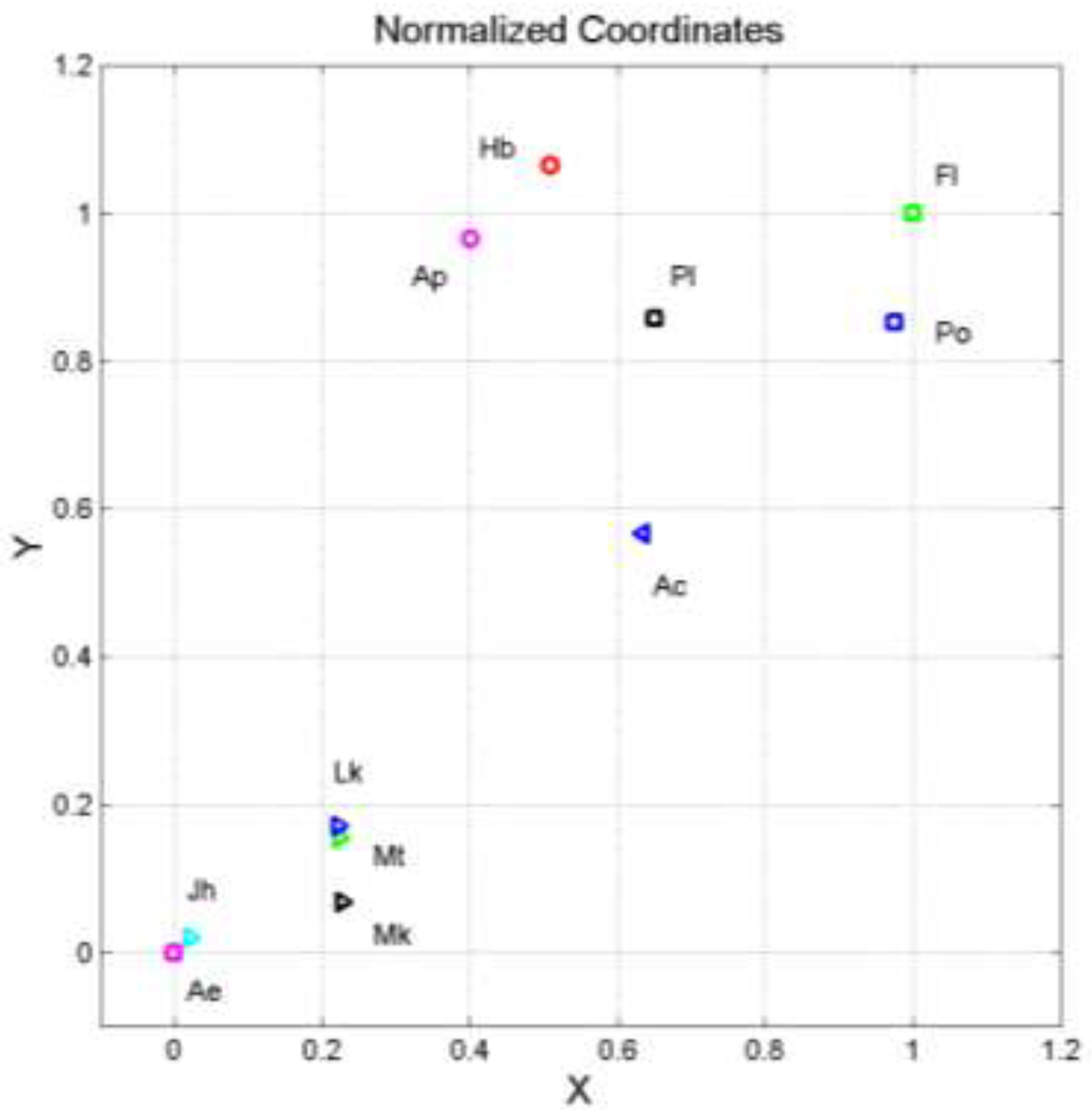
Figure 2.
Scatterplots and regression lines between (words, independent variable) and (sentences, dependent variable) in the following texts: Matthew (green triangles and green line); Mark (black triangles and black line); Luke (blue triangles and blue line); John (cyan triangles and cyan line).
Figure 2.
Scatterplots and regression lines between (words, independent variable) and (sentences, dependent variable) in the following texts: Matthew (green triangles and green line); Mark (black triangles and black line); Luke (blue triangles and blue line); John (cyan triangles and cyan line).
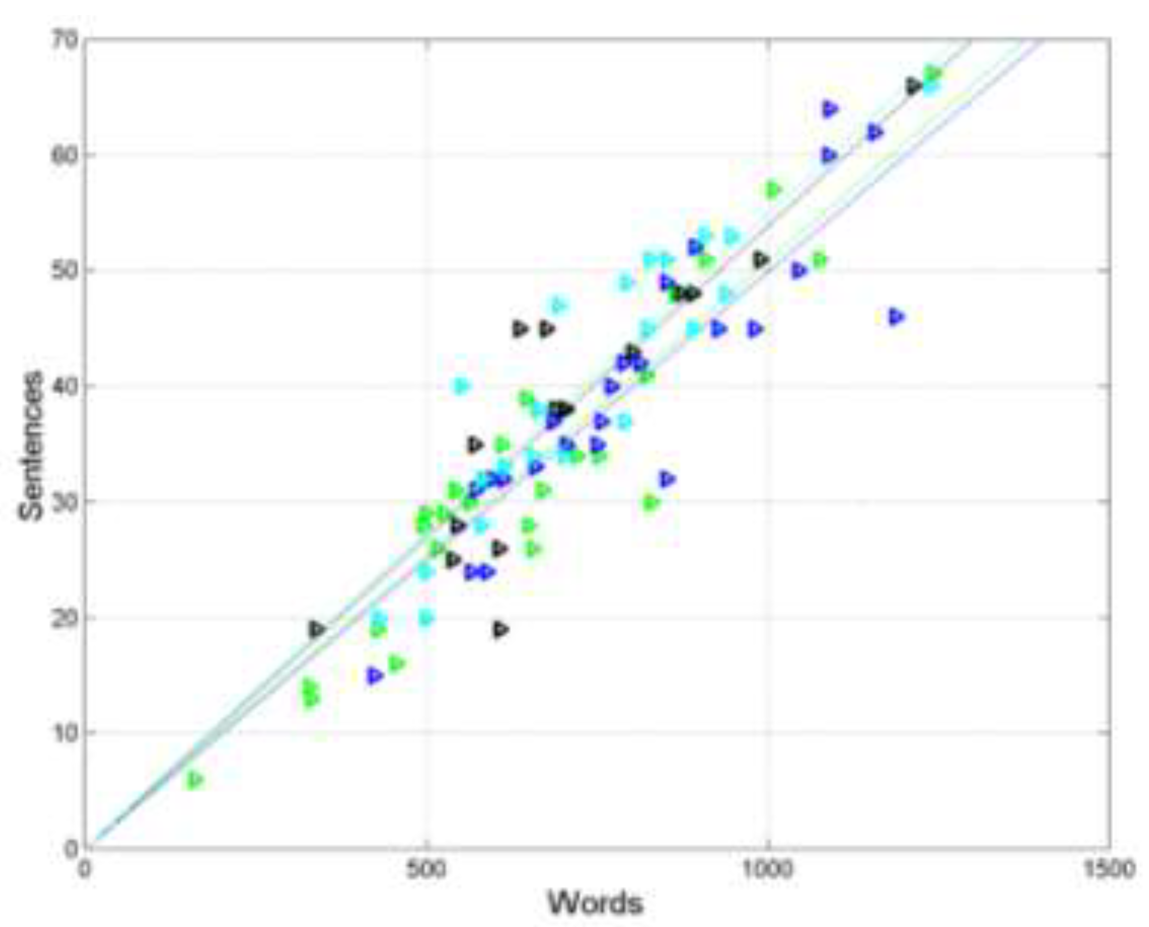
Figure 3.
Scatterplots and regression lines between (words, independent variable) and (sentences, dependent variable) in the following texts: Matthew (green triangles and green line); Acts (blue circles and blue line); Hebrews (red circles and red line); Apocalypse (magenta circles and magenta line). The magenta line (Apocalypse) and the red line (Hebrews) are superposed because they practically coincide (see Table 3).
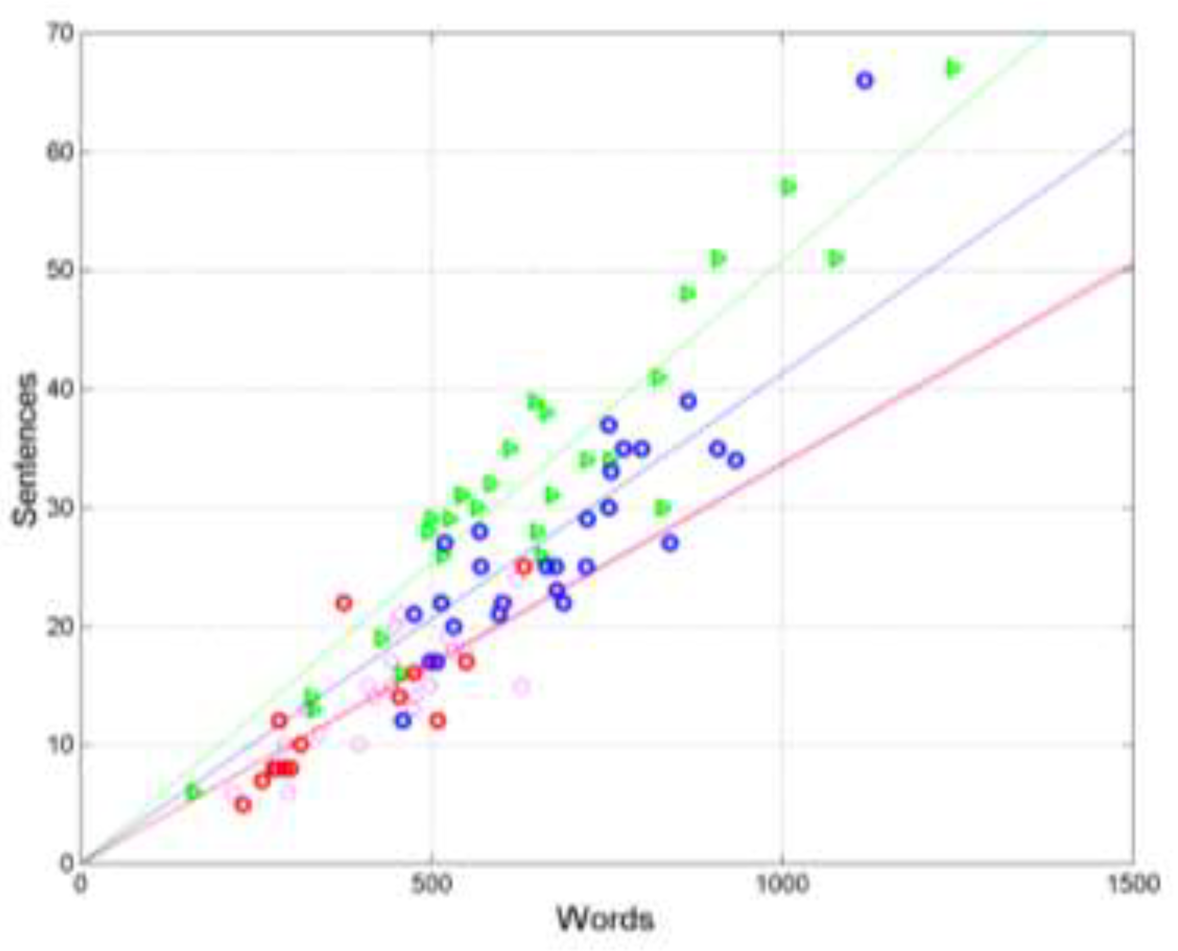
Figure 4.
Scatterplots and regression lines between (sentences, independent variable) and (interpunctions, dependent
variable) in the following texts: Matthew (green triangles and green line); Mark (black triangles and black line);
Luke (blue triangles and blue line); John (cyan triangles and cyan line).
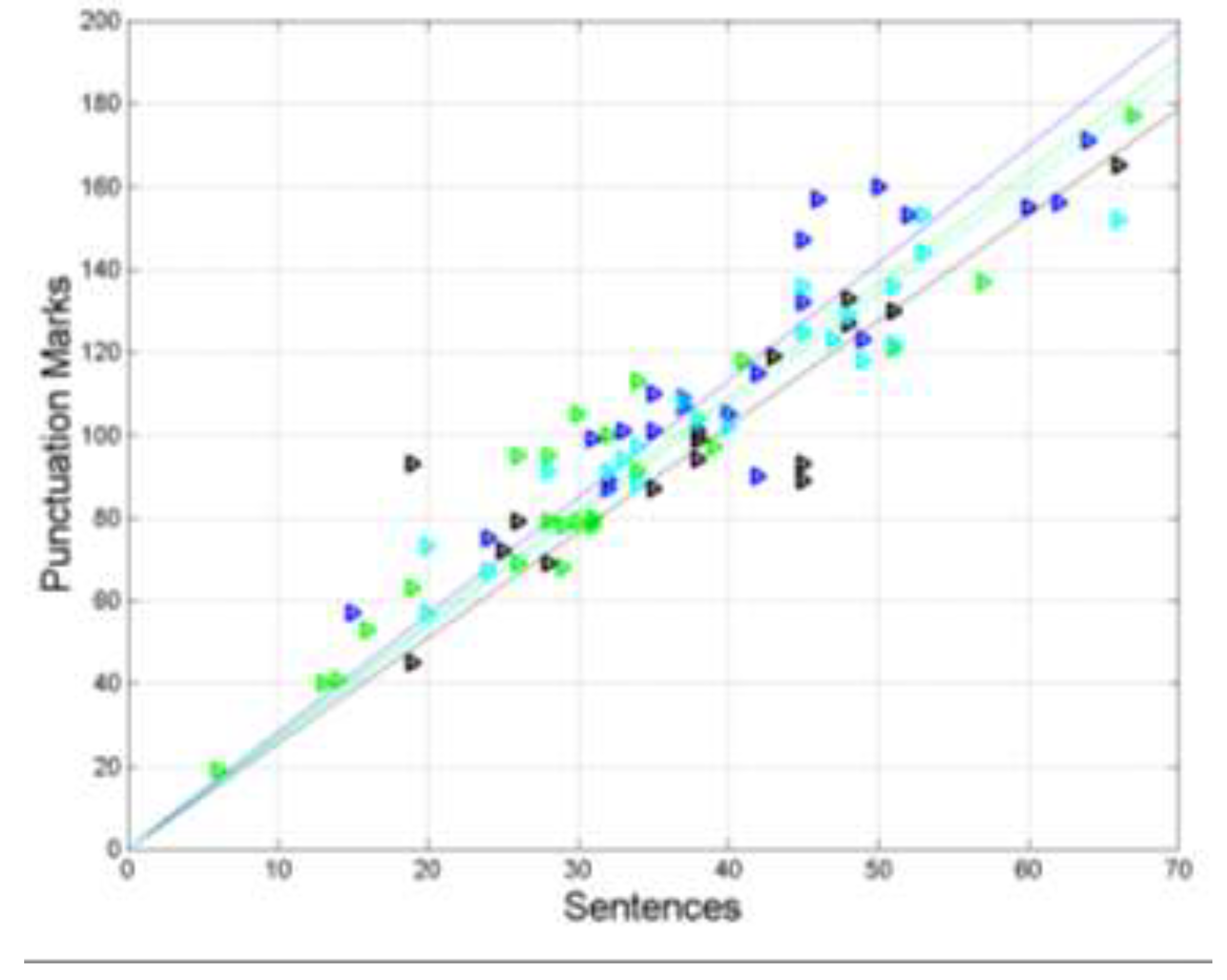
Figure 5.
Scatterplots and regression lines between (sentences, independent variable) and (interpunctions, dependent variable) in the following texts: Matthew (green triangles and green line); Acts (blue circles and blue line); Hebrews (red circles and red line); Apocalypse (magenta circles and magenta line). The green line (Matthew) and the blue line (Acts) are superposed because they practically coincide (see Table 3).
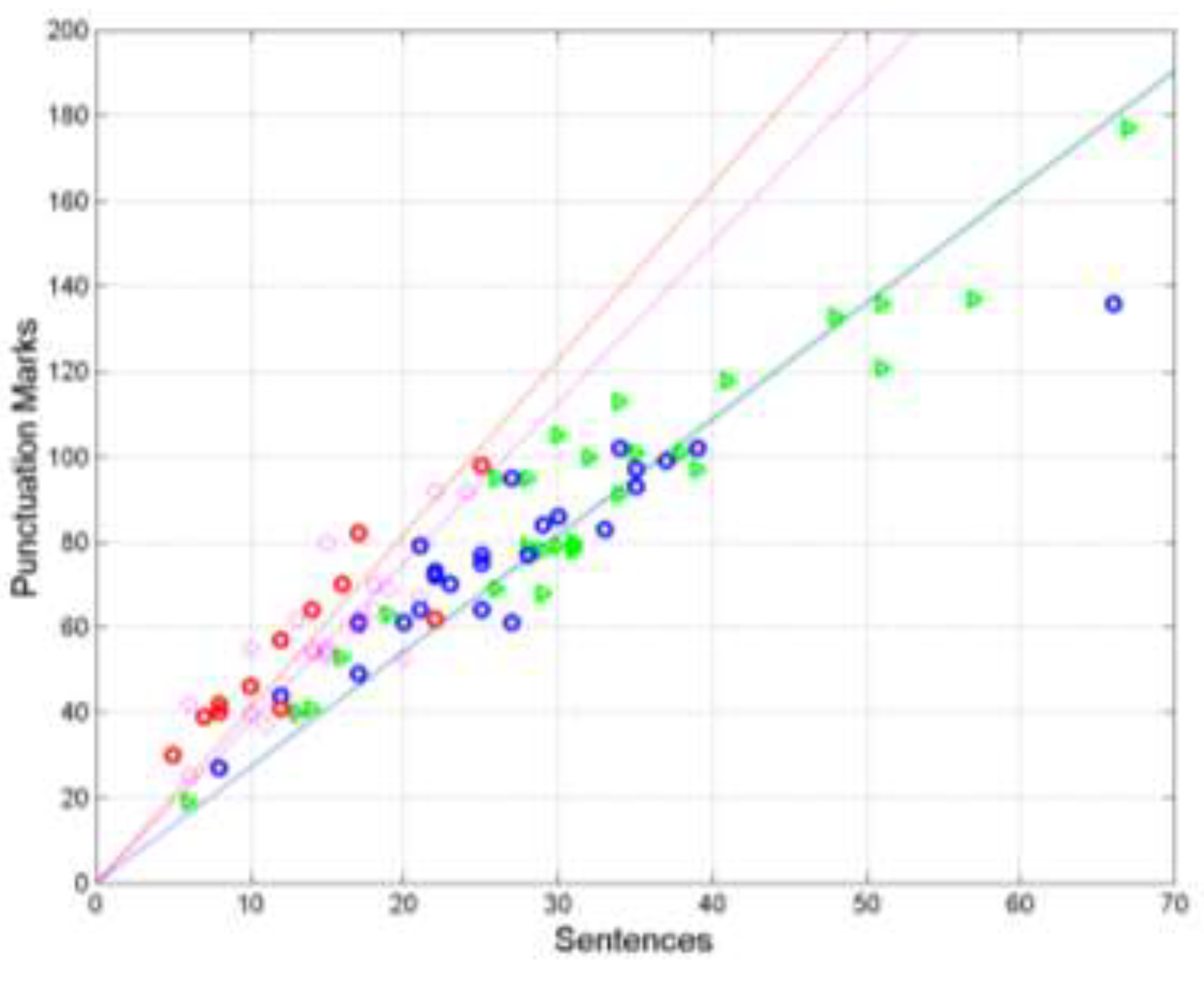
Figure 6.
Scatterplots and regression lines between (words, independent variable) and (sentences, dependent variable) in John (cyan triangles and cyan) and in Aesop (magenta circles and magenta line). Notice that the two regression lines are practically superposed and the scattering of the two sets are very alike.
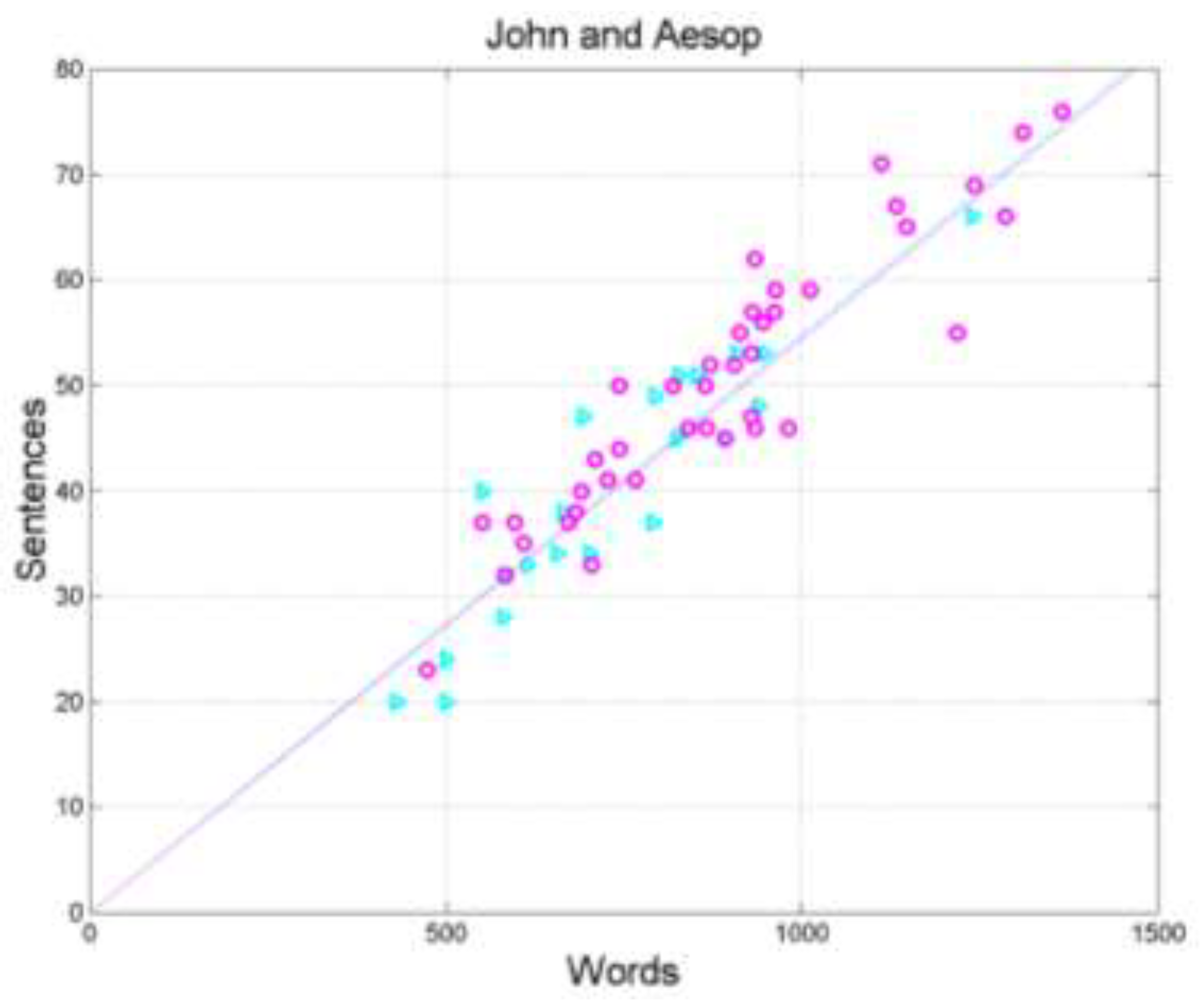
Figure 7.
Scatterplots and regression lines between (sentences, independent variable) and (interpunctions, dependent variable) in John (cyan triangles and cyan) and in Aesop (magenta circles and magenta line).
Figure 7.
Scatterplots and regression lines between (sentences, independent variable) and (interpunctions, dependent variable) in John (cyan triangles and cyan) and in Aesop (magenta circles and magenta line).
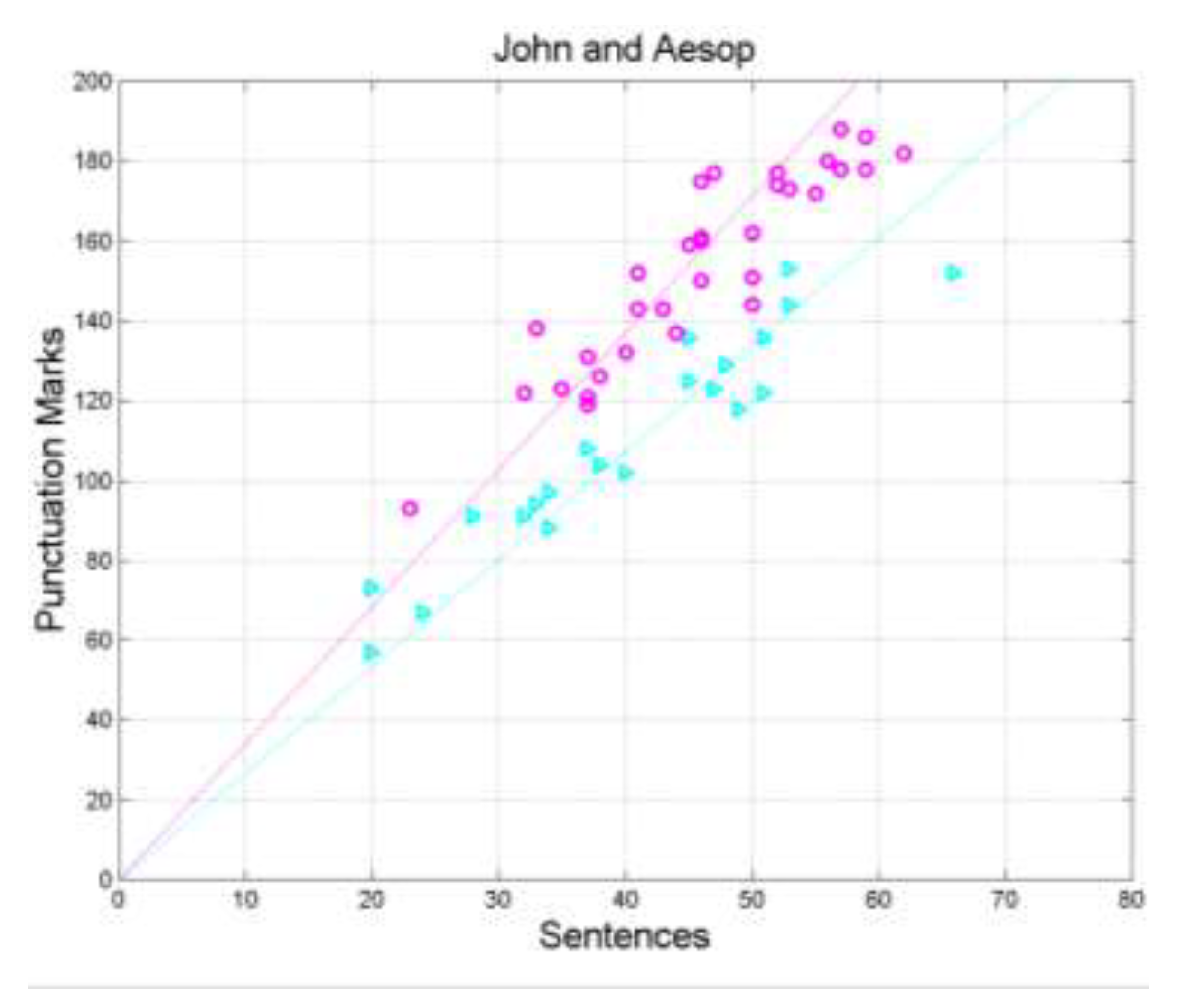
Figure 8.
and for each NT input texts indicated in abscissa. Upper panel: S‒channel; Lower panel: I‒channel. Output texts: Matthew: black; Mark: yellow; Luke: blue; John: green; Acts: cyan; Hebrews: red; Apocalypse: magenta. Mean and standard deviation numerical values are reported in Appendix A. Notice that .
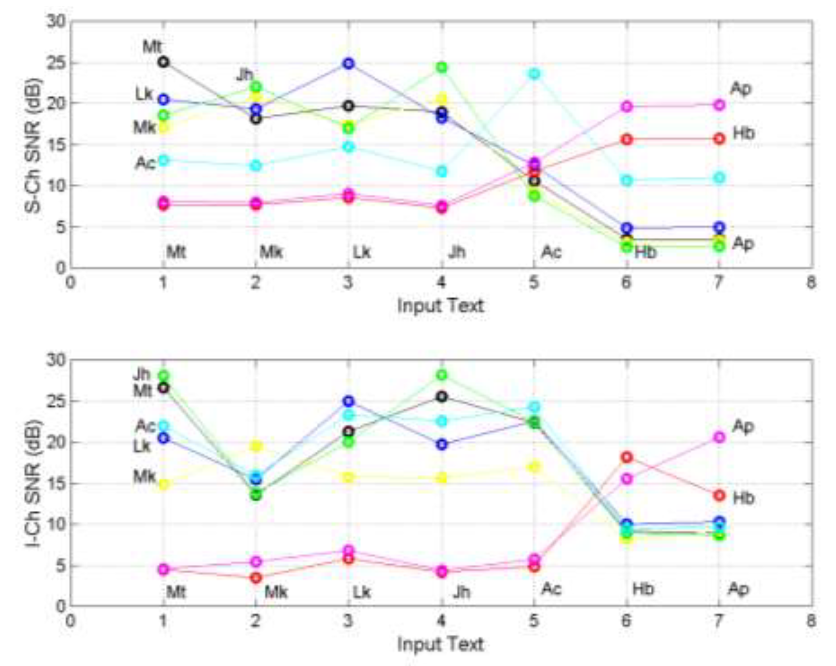
Figure 9.
S‒channel. (a) Scatterplot of versus in S‒channels; (b) Scatterplot of versus . Matthew (green triangles); Mark (black triangles); Luke (blue triangles); John (cyan triangles); Acts (blues circles); Hebrews (red circles); Apocalypse (magenta circles).
Figure 9.
S‒channel. (a) Scatterplot of versus in S‒channels; (b) Scatterplot of versus . Matthew (green triangles); Mark (black triangles); Luke (blue triangles); John (cyan triangles); Acts (blues circles); Hebrews (red circles); Apocalypse (magenta circles).
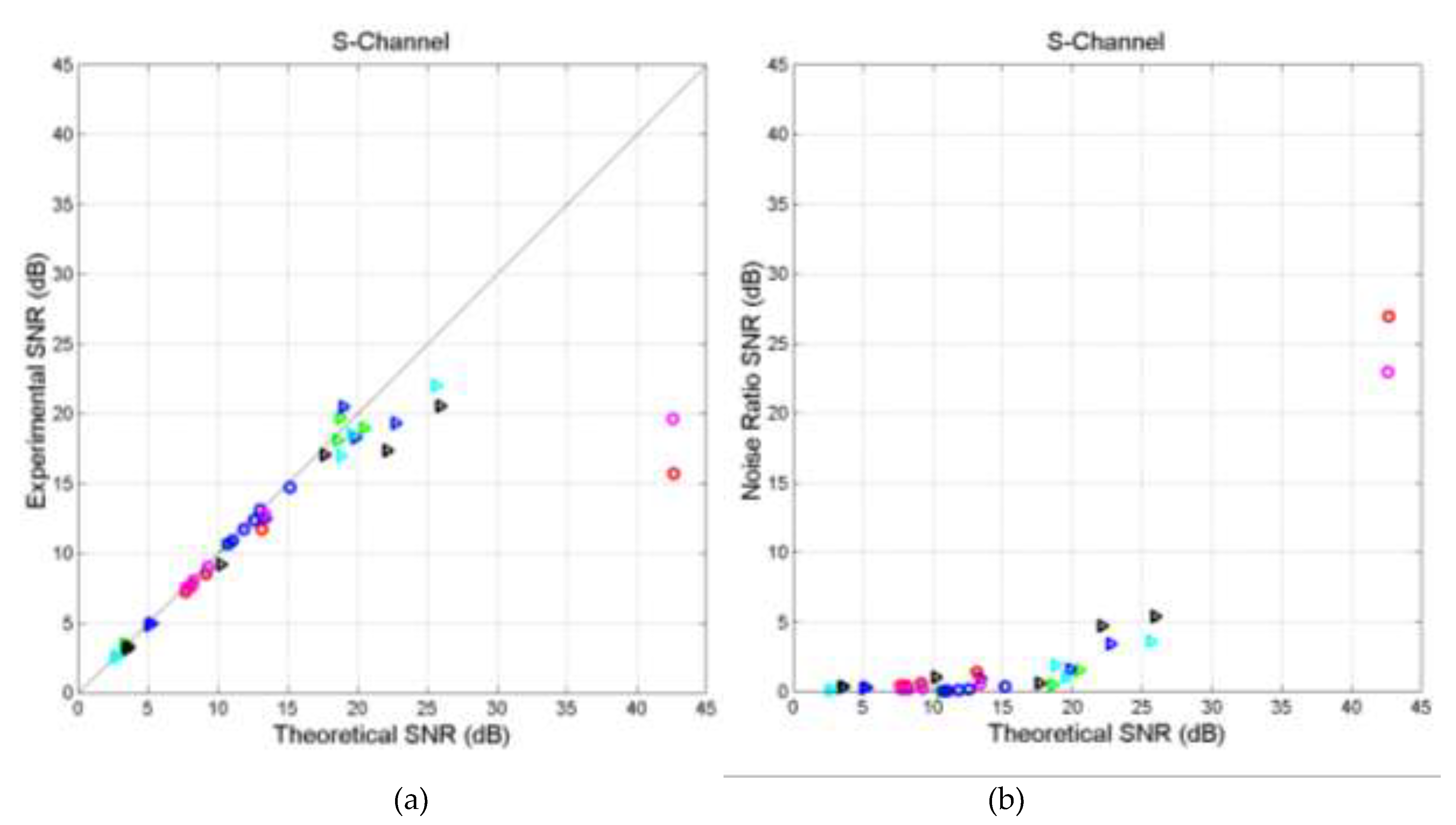
Figure 10.
I‒channel. (a) Scatterplot of versus in S‒channels; (b) Scatterplot of versus . Matthew (green triangles); Mark (black triangles); Luke (blue triangles); John (cyan triangles); Acts (blues circles); Hebrews (red circles); Apocalypse (magenta circles).
Figure 10.
I‒channel. (a) Scatterplot of versus in S‒channels; (b) Scatterplot of versus . Matthew (green triangles); Mark (black triangles); Luke (blue triangles); John (cyan triangles); Acts (blues circles); Hebrews (red circles); Apocalypse (magenta circles).
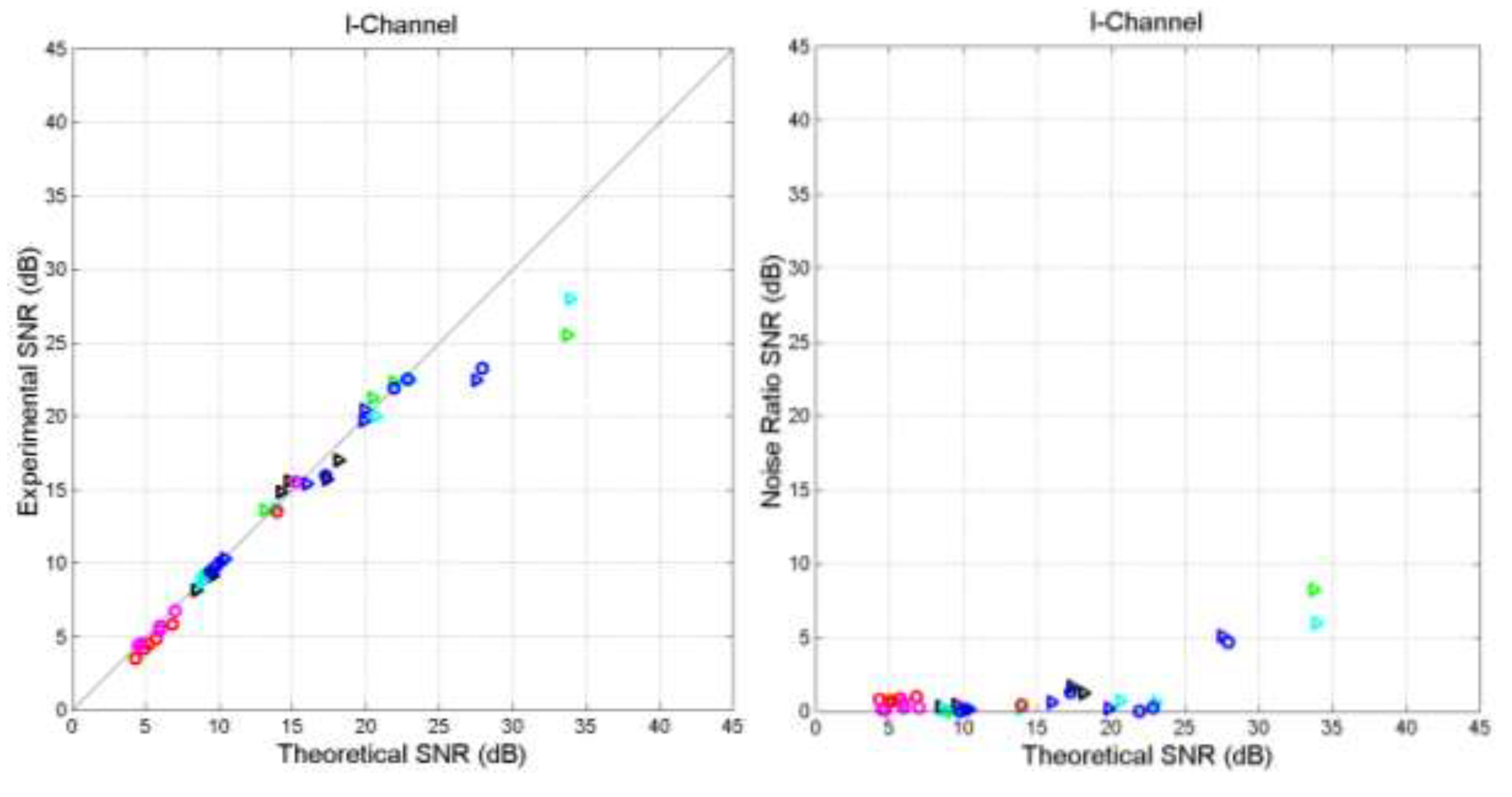
Figure 11.
Matching texts in S-channels and in I-channels.
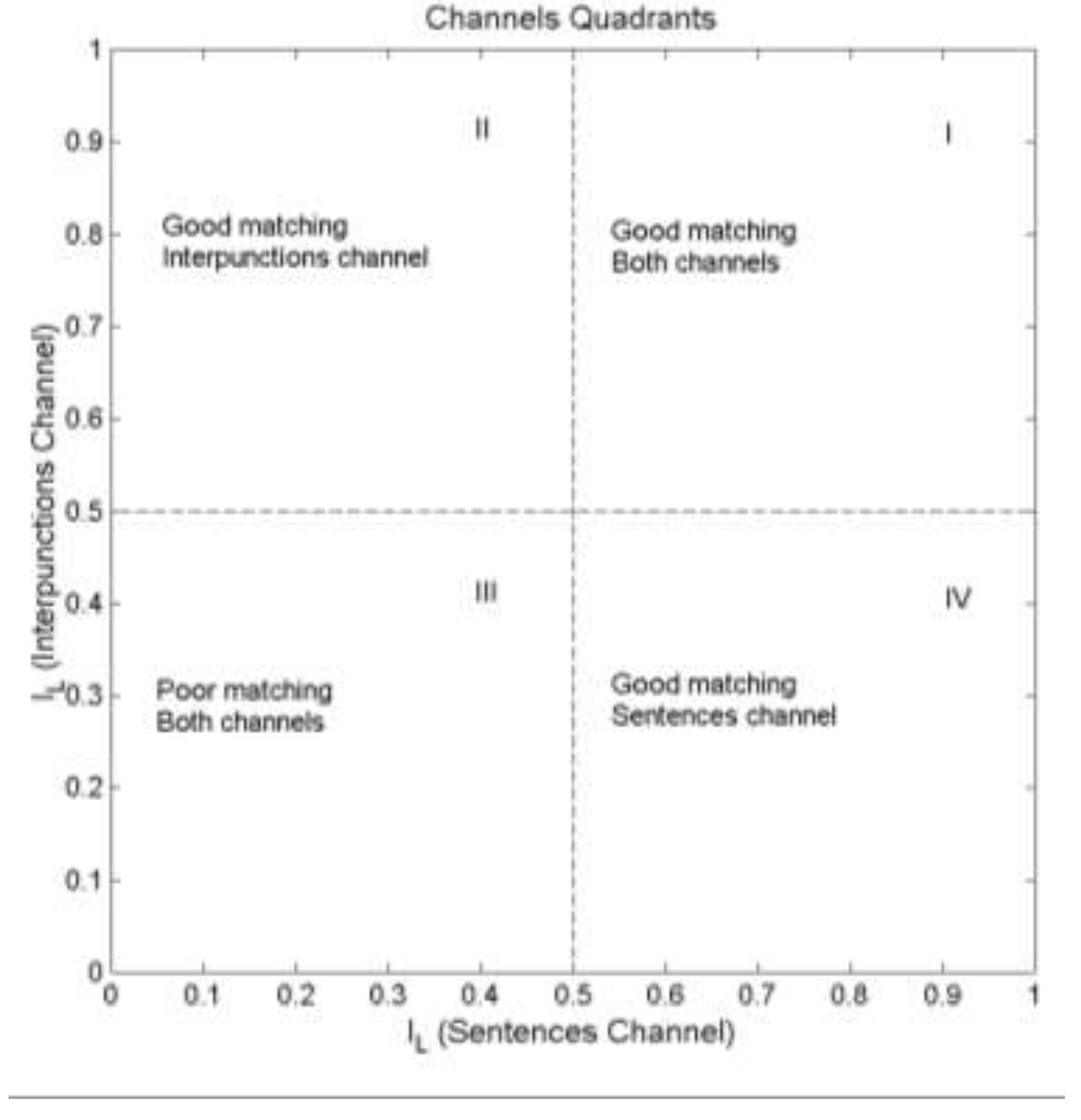
Figure 12.
Scatterplot of of the Interpunctions channel (ordinate scale) versus of the S‒channel (abscissa scale). Output channels (first line in Table 11 and Table 12): Matthew: black circles; Mark: yellow; Luke: blue; John: green; Acts: cyan; Hebrews: red; Apocalypse: magenta. Percentages indicate the relative number of cases falling in a quadrant.
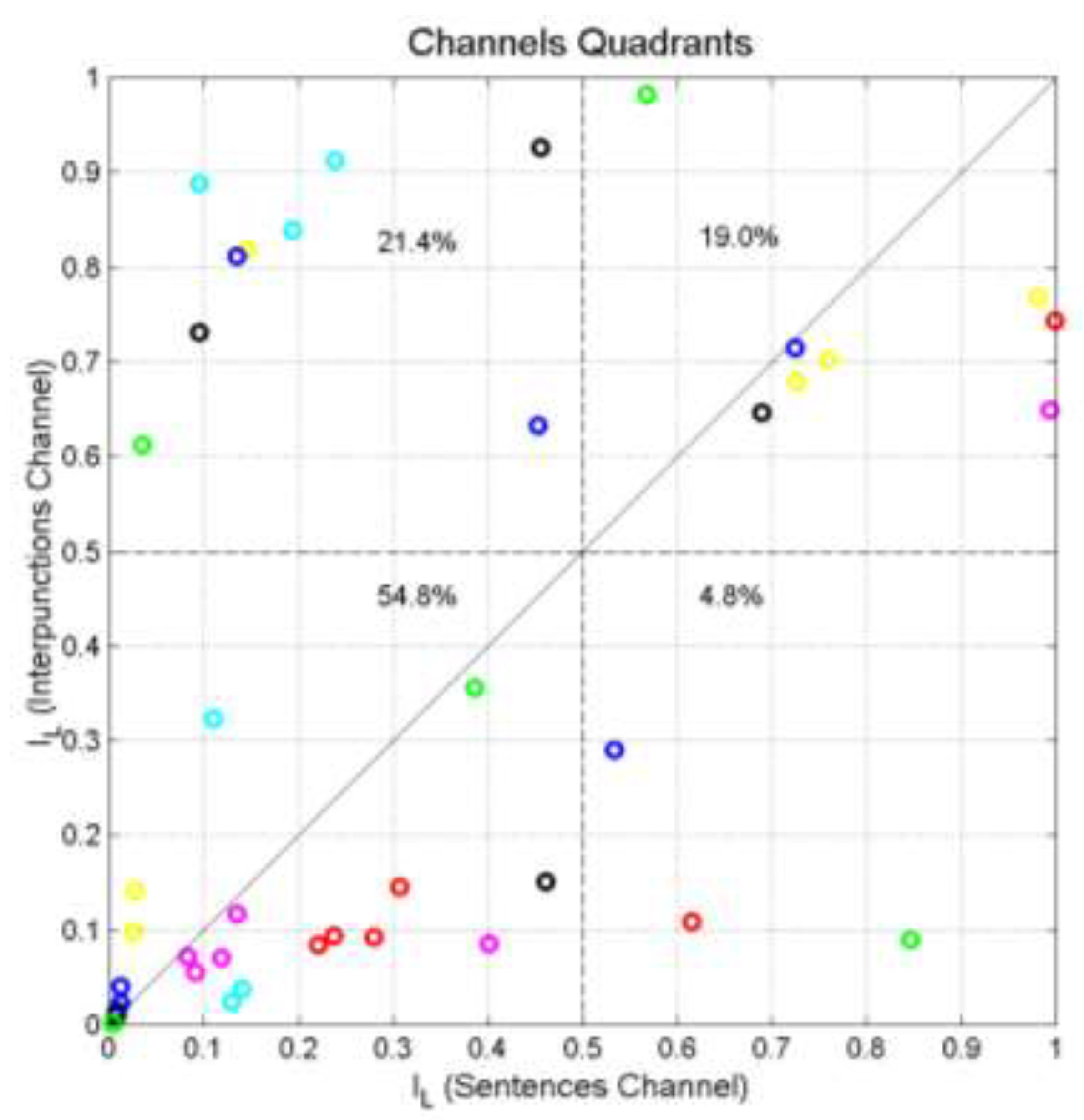
Figure 13.
Scatterplot of of S‒channel and I‒channel versus . Matthew (green triangles); Mark (black triangles); Luke (blue triangles); John (cyan triangles); Acts (blues circles); Hebrews (red circles); Apocalypse (magenta circles). The black line draws Equation (15).
Figure 13.
Scatterplot of of S‒channel and I‒channel versus . Matthew (green triangles); Mark (black triangles); Luke (blue triangles); John (cyan triangles); Acts (blues circles); Hebrews (red circles); Apocalypse (magenta circles). The black line draws Equation (15).
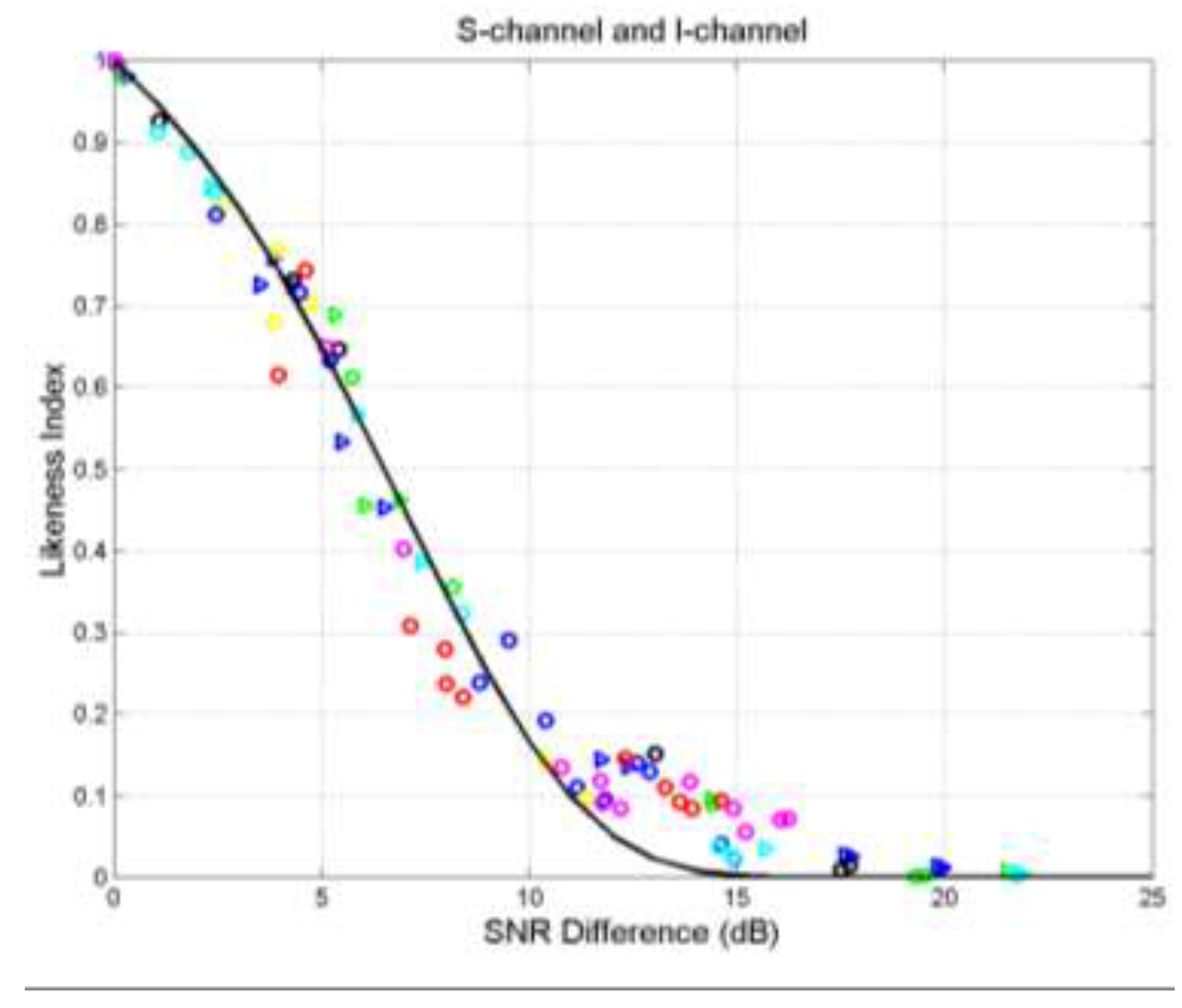
Table 1.
New Testament. Mean values (averaged over all chapters) of (characters per word), (words per sentence), (interpunctions per sentencewords per interpunctions) and (universal readability index). The genealogy in Matthew (verses 1.1‒1.17) and in Luke (verses 3.23‒3.38) have been deleted for not biasing the statistical analyses. All parameters have been computed by weighting a chapter with the fraction of total words of the literary text.
| Book | Total Words | |||||
|---|---|---|---|---|---|---|
| Matthew | 18,121 | 4.91 | 20.27 | 2.83 | 7.18 | 53.90 |
| Mark | 11,393 | 4.96 | 19.14 | 2.68 | 7.17 | 54.87 |
| Luke | 19,384 | 4.91 | 20.47 | 2.89 | 7.11 | 54.21 |
| John | 15,503 | 4.54 | 18.56 | 2.74 | 6.79 | 57.65 |
| Acts | 18,757 | 5.10 | 25.47 | 2.91 | 8.77 | 41.37 |
| Hebrews | 4,940 | 5.33 | 32.00 | 4.53 | 7.02 | 53.10 |
| Apocalypse | 9,870 | 4.66 | 30.70 | 3.97 | 7.79 | 49.46 |
Table 2.
Greek Literature. Mean values (averaged over all chapters) of (characters per word), (words per sentence), (interpunctions per sentencewords per interpunctions, or words interval) and the corresponding (universal readability index). All parameters have been computed by weighting a chapter with the fraction of total words of the literary text.
| Author | Total Words | |||||
|---|---|---|---|---|---|---|
| Aesop (620–564 BC, Fables) | 39,122 | 5.24 | 18.29 | 3.46 | 5.28 | 64.95 |
| Polybius (200‒118 BC, The Histories) | 256,495 | 5.97 | 29.19 | 3.30 | 8.88 | 37.22 |
| Flavius Josephus (37‒100 AD, The Jewish War) | 121,717 | 5.51 | 31.05 | 3.20 | 9.74 | 31.44 |
| Plutarch (46‒119 AD, Parallel Lives) | 499,683 | 5.51 | 29.35 | 3.73 | 7.82 | 43.53 |
Table 3.
Slope and the correlation coefficient of the regression lines of versus , and versus in the indicated texts. Four decimal digits are reported because some values differ only from the third digit. These parameters are calculated by uniformly weighing each block text, e.g. weight in Matthew.
Table 3.
Slope and the correlation coefficient of the regression lines of versus , and versus in the indicated texts. Four decimal digits are reported because some values differ only from the third digit. These parameters are calculated by uniformly weighing each block text, e.g. weight in Matthew.
| Text | ||||
|---|---|---|---|---|
| Matthew | 0.0508 | 0.9410 | 2.7271 | 0.9548 |
| Mark | 0.0538 | 0.8985 | 2.5527 | 0.8800 |
| Luke | 0.0499 | 0.8975 | 2.8296 | 0.9243 |
| John | 0.0549 | 0.9181 | 2.6797 | 0.9517 |
| Acts | 0.0413 | 0.8807 | 2.7192 | 0.9280 |
| Hebrews | 0.0336 | 0.8037 | 4.0970 | 0.9005 |
| Apocalypse | 0.0338 | 0.8063 | 3.7605 | 0.8173 |
Table 4.
Theoretical slope and correlation coefficient of the regression line according to Section 4, for the indicated input texts. Output Channel: Matthew.
Table 4.
Theoretical slope and correlation coefficient of the regression line according to Section 4, for the indicated input texts. Output Channel: Matthew.
| Text | Sentences versus Sentences | Interpunctions versus Interpunctions | ||
|---|---|---|---|---|
| Mark | 0.9442 | 0.9940 | 1.0683 | 0.9814 |
| Luke | 1.0180 | 0.9938 | 0.9638 | 0.9960 |
| John | 0.9253 | 0.9981 | 1.0177 | 0.9999 |
| Acts | 1.2300 | 0.9890 | 1.0029 | 0.9968 |
| Hebrews | 1.5119 | 0.9576 | 0.6656 | 0.9891 |
| Apocalypse | 1.5030 | 0.9589 | 0.7252 | 0.9516 |
Table 5.
S‒channel. Theoretical signal–to–noise ratio (dB) in the channel between the (input) text indicated in the first column and the (output) text indicated in the first line. For example, if the input is Matthew and the output is Mark, then ; vice versa if the input is Mark and the output is Matthew, then .
| Text | Matthew | Mark | Luke | John | Acts | Hebrews | Apocalypse |
|---|---|---|---|---|---|---|---|
| Matthew | 17.70 | 19.06 | 19.56 | 13.04 | 8.12 | 8.22 | |
| Mark | 18.59 | 22.79 | 25.66 | 12.61 | 8.12 | 8.21 | |
| Luke | 18.76 | 22.14 | 18.87 | 15.14 | 9.14 | 9.26 | |
| John | 20.50 | 25.99 | 19.87 | 11.83 | 7.67 | 7.76 | |
| Acts | 10.62 | 10.26 | 13.44 | 9.15 | 13.13 | 13.36 | |
| Hebrews | 3.29 | 3.48 | 5.10 | 2.61 | 10.75 | 42.61 | |
| Apocalypse | 3.46 | 3.64 | 5.29 | 2.77 | 11.04 | 42.68 |
Table 6.
I‒channel. Theoretical signal–to–noise ratio (dB) in the channel between the (input) text indicated in the first column and the (output) text indicated in the first line. For example, if the input is Matthew and the output is Mark, then , vice versa if the input is Mark and the output is Matthew, then .
| Text | Matthew | Mark | Luke | John | Acts | Hebrews | Apocalypse |
|---|---|---|---|---|---|---|---|
| Matthew | 14.25 | 19.94 | 33.94 | 21.94 | 5.19 | 4.66 | |
| Mark | 13.16 | 16.02 | 13.96 | 17.23 | 4.30 | 5.94 | |
| Luke | 20.53 | 17.37 | 20.70 | 27.93 | 6.82 | 7.02 | |
| John | 33.75 | 14.78 | 19.91 | 22.81 | 4.89 | 4.51 | |
| Acts | 21.89 | 18.20 | 27.56 | 23.06 | 5.73 | 5.96 | |
| Hebrews | 9.15 | 8.45 | 10.12 | 8.93 | 9.39 | 15.25 | |
| Apocalypse | 8.85 | 9.60 | 10.45 | 8.80 | 9.75 | 13.92 |
Table 7.
Theoretical slope and correlation coefficient of the regression line according to Section 4, for the indicated input texts. Output Channel: Hebrews. Notice that 5 decimal digits are reported for Apocalypse because its value is very close to 1.
Table 7.
Theoretical slope and correlation coefficient of the regression line according to Section 4, for the indicated input texts. Output Channel: Hebrews. Notice that 5 decimal digits are reported for Apocalypse because its value is very close to 1.
| Text | Sentences vs Sentences | % | Interpunctions vs Interpunctions | ||
|---|---|---|---|---|---|
| Matthew | 0.6614 | 0.9576 | 1.5023 | 0.9891 | |
| Mark | 0.6245 | 0.9833 | 1.6050 | 0.9990 | |
| Luke | 0.6733 | 0.9837 | 1.4479 | 0.9983 | |
| John | 0.6120 | 0.9737 | 1.5289 | 0.9905 | |
| Acts | 0.8136 | 0.9897 | 1.5067 | 0.9977 | |
| Apocalypse | 0.9941 | 0.99999 | 1.0895 | 0.9865 | |
Table 8.
Theoretical slope and correlation coefficient of the regression line according to Section 4, for the indicated input texts. Output Channel: Apocalypse. Notice that 5 decimal digits are reported for Hebrews because its value is very close to 1.
Table 8.
Theoretical slope and correlation coefficient of the regression line according to Section 4, for the indicated input texts. Output Channel: Apocalypse. Notice that 5 decimal digits are reported for Hebrews because its value is very close to 1.
| Text | Sentences vs Sentences | Interpunctions vs Interpunctions | ||
|---|---|---|---|---|
| Matthew | 0.6654 | 0.9589 | 1.3789 | 0.9516 |
| Mark | 0.6283 | 0.9841 | 1.4731 | 0.9929 |
| Luke | 0.6774 | 0.9845 | 1.3290 | 0.9754 |
| John | 0.6157 | 0.9747 | 1.4033 | 0.9547 |
| Acts | 0.8184 | 0.9903 | 1.3829 | 0.9731 |
| Hebrews | 1.0060 | 0.99999 | 0.9179 | 0.9865 |
Table 9.
Slope and the correlation coefficient of the regression lines between versus , and versus for the indicated texts of the Greek Literature. Slope and correlation coefficients have been calculated as those reported in Table xx.
Table 9.
Slope and the correlation coefficient of the regression lines between versus , and versus for the indicated texts of the Greek Literature. Slope and correlation coefficients have been calculated as those reported in Table xx.
| Author | ||||
|---|---|---|---|---|
| Polybius | 0.0343 | 0.9971 | 3.2432 | 0.9885 |
| Plutarch | 0.0371 | 0.9195 | 3.3539 | 0.9577 |
| Flavius Josephus | 0.0325 | 0.9734 | 3.1891 | 0.9846 |
| Aesop | 0.0545 | 0.9032 | 3.4236 | 0.9302 |
| John | 0.0549 | 0.9181 | 2.6797 | 0.9517 |
Table 10.
S‒channel, Greek Literature. Theoretical signal–to–noise ratio (dB) in the channel between the (input) text indicated in the first column and the (output) text indicated in the first line. For example, if the input is Polybius and the output is Plutarch, then ; vice versa if the input is Plutarch and the output is Polybius, then .
| Text | Polybius | Plutarch | Flavius | Aesop | John |
|---|---|---|---|---|---|
| Polybius | 8.48 | 16.08 | 1.42 | 1.78 | |
| Plutarch | 9.81 | 14.12 | 6.51 | 6.38 | |
| Flavius Josephus | 15.19 | 12.24 | 2.30 | 2.47 | |
| Aesop | 7.08 | 9.89 | 7.46 | 28.61 | |
| John | 7.28 | 9.78 | 7.51 | 28.74 |
Table 11.
I‒channel, Greek Literature. Theoretical signal–to–noise ratio (dB) in the channel between the (input) text indicated in the first column and the (output) text indicated in the first line. For example, if the input is Polybius and the output is Plutarch, then ; vice versa if the input is Plutarch and the output is Polybius, then .
| Text | Polybius | Plutarch | Flavius | Aesop | John |
|---|---|---|---|---|---|
| Polybius | 16.49 | 30.80 | 12.15 | 13.19 | |
| Plutarch | 17.06 | 18.32 | 21.07 | 13.91 | |
| Flavius Josephus | 30.56 | 17.51 | 12.77 | 14.11 | |
| Aesop | 13.07 | 21.42 | 13.94 | 13.04 | |
| John | 10.84 | 11.94 | 12.02 | 10.77 |
Table 12.
Average value of in S‒channels. For example, in the channels HebrewsApocalypse, from Appendix B we get the average value . In bold type the cases in which .
Table 12.
Average value of in S‒channels. For example, in the channels HebrewsApocalypse, from Appendix B we get the average value . In bold type the cases in which .
| Mt | Mk | Lk | Jh | Ac | Hb | Ap | |
|---|---|---|---|---|---|---|---|
| Mt | 1 | ||||||
| Mk | 0.160 | 1 | |||||
| Lk | 0.707 | 0.630 | 1 | ||||
| Jh | 0.511 | 0.914 | 0.419 | 1 | |||
| Ac | 0.145 | 0.128 | 0.188 | 0.066 | 1 | ||
| Hb | 0.144 | 0.132 | 0.160 | 0.133 | 0.372 | 1 | |
| Ap | 0.063 | 0.059 | 0.074 | 0.044 | 0.271 | 0.996 | 1 |
Table 13.
Average value of in I‒channels. In bold type the cases in which .
| Mt | Mk | Lk | Jh | Ac | Hb | Ap | |
|---|---|---|---|---|---|---|---|
| Mt | 1 | ||||||
| Mk | 0.427 | 1 | |||||
| Lk | 0.681 | 0.485 | 1 | ||||
| Jh | 0.954 | 0.429 | 0.494 | 1 | |||
| Ac | 0.785 | 0.571 | 0.863 | 0.750 | 1 | ||
| Hb | 0.051 | 0.096 | 0.084 | 0.037 | 0.067 | 1 | |
| Ap | 0.043 | 0.099 | 0.079 | 0.037 | 0.062 | 0.697 | 1 |
Table 14.
Overall total average value of . For example, in the channels HebrewsApocalypse, from Tables 12,13 we get the average value . In bold type the cases in which .
Table 14.
Overall total average value of . For example, in the channels HebrewsApocalypse, from Tables 12,13 we get the average value . In bold type the cases in which .
| Mt | Mk | Lk | Jh | Ac | Hb | Ap | |
|---|---|---|---|---|---|---|---|
| Mt | 1 | ||||||
| Mk | 0.294 | 1 | |||||
| Lk | 0.694 | 0.558 | 1 | ||||
| Jh | 0.733 | 0.674 | 0.457 | 1 | |||
| Ac | 0.465 | 0.350 | 0.526 | 0.408 | 1 | ||
| Hb | 0.098 | 0.114 | 0.122 | 0.085 | 0.220 | 1 | |
| Ap | 0.053 | 0.079 | 0.077 | 0.041 | 0.167 | 0.847 | 1 |
Disclaimer/Publisher’s Note: The statements, opinions and data contained in all publications are solely those of the individual author(s) and contributor(s) and not of MDPI and/or the editor(s). MDPI and/or the editor(s) disclaim responsibility for any injury to people or property resulting from any ideas, methods, instructions or products referred to in the content. |
© 2023 by the authors. Licensee MDPI, Basel, Switzerland. This article is an open access article distributed under the terms and conditions of the Creative Commons Attribution (CC BY) license (http://creativecommons.org/licenses/by/4.0/).
Copyright: This open access article is published under a Creative Commons CC BY 4.0 license, which permit the free download, distribution, and reuse, provided that the author and preprint are cited in any reuse.


