Theorem on the Structure of the Fractionally Linear Functional Extremal Function

1. Introduction. Statement of the problem

Currently, there are many practical models of reliability, mass maintenance, and security that are adequately described by a semi-Markov controlled process (MCP) with a finite set of states.

In these models, control consists in choosing the moments of intervention in the system operation (for example, preventive repair, replacement of failed or worn out units, frequency of determination of the current state of the system). If the studied models consider a class of randomized control strategies, then we come to the problem of functional analysis: the search for an extremum of some functional characterizing the quality of control on the set of probability measures (distributions) defining the randomized strategy. The result stated in the paper allows to simplify the problem (if probabilistic measures are defined on a straight line or a semi-straight line) by reducing it to the problem of mathematical analysis (the problem of finding an extremum of some function over a set of parameters), which, in principle, allows to use software tools and to bring the result to a number.

$$I\left(G\right)=\frac{{\int }_{u\in U}A\left(u\right)G\left(du\right)}{{\int }_{u\in U}B\left(u\right)G\left(du\right)}$$

(1)

on some admissible set of probability measures $\Omega$ (the set of Markov homogeneous randomized control strategies) and the definition of the probability measure on which this extremum is reached [1].

For controllable models of mass service, reliability and safety, when it comes to the optimal choice of service duration or periodicity of restoration work, the control space coincides with the set of positive numbers $U=R^{+}=\left[0,\mathrm{\infty }\right],$ and the probability measure is given by distribution functions $g=G\left(u\right)=P\left\{\zeta <u\right\}{,}^{ }G\left(0\right)=0,$ where $\zeta$ is the decision to be made.

Let us introduce two distribution functions

$$\begin{gathered} g=G_1\left(u\right),g=G_2\left(u\right), \\ 0\le G_1\left(u\right)\le G_2\left(u\right)\le 1{,}^{ }u\ge 0, \\ {G}_1\left(0\right)=G_2\left(0\right)=0{,}^{ }u\le 0, \end{gathered}$$

and define the set of admissible distributions

$$\Omega =\left\{G:G_1\left(u\right)\le G\left(u\right)\le G_2\left(u\right),u\ge 0\right\},$$

(2)

Now in the accepted notations we can formulate the main mathematical problem: to determine the maximum of fractionally linear functional (1) over the set of admissible distributions (2) and the strategy (distribution) $G^{\mathrm{*}}$ on which this maximum is reached,

$$\underset{G\in \Omega }{max}I\left(G\right)=I\left(G_{ }^{\mathrm{*}}\right).$$

(3)

Note that the constraints (2) can be represented as constraints of the type of inequalities on linear functionals

$$G_1\left(u\right)\le {\int }_0^{+\mathrm{\infty }}\phi \left(x,u\right)dG\left(x\right)\le G_2\left(u\right),\phi \left(x,u\right)=\left\{\begin{array}{c}1,x<u,\\ 0,x\ge u,\end{array}\right.u\in \left[0,+\mathrm{\infty }\right).$$

Consequently, the formulated problem is a fractionally linear programming problem with an uncountable number of linear constraints.

If we use the lemma [2] on the coincidence of the sets of probability measures on which the extremum of a fractionally linear functional and the extremum of a specially chosen linear functional are reached, the problem can be simplified by reducing it to the linear case.

Here is the formulation of this lemma.

Lemma 1.

If there exists a maximum of a fractionally linear functional$I\left(G\right)$on some set$\Omega$

$$\underset{G\in \Omega }{max}I\left(G\right)=C,$$

then the equality of the sets

$$\left\{G:I\left(G\right)=C\right\}=\left\{G:{\int }_{u\in U}С\left(u\right)G\left(du\right)=0\right\},$$

where$U$is the set of possible controls, and the integrand function$С\left(u\right)$is defined by equality$С\left(u\right)=А\left(u\right)-СB\left(u\right)$ , and for the linear functional${\int }_{u\in U}С\left(u\right)G\left(du\right)$the following relation is correct

$$\underset{G\in \Omega }{max}{\int }_{u\in U}С\left(u\right)G\left(du\right)=0.$$

Thus, if it is found that for some probability measure, a certain structure, the extremum of the linear functional is reached and all probability measures, of the given structure, belong to the set $\Omega$then the extremum of the fractionally linear functional can be sought over a narrower set. Moreover, if each probabilistic measure of a selected structure is uniquely defined by parameters (for example, measures defined on a discrete set), then the problem of functional analysis is reduced to the problem of finding an extremum of a function in the parameter space.

Here it should be noted that the integrand function of a linear functional depends on an unknown parameter, and this creates certain difficulties when studying the structure of extreme probability measures.

2. Theorem on the structure of the extremal function

Let us formulate the requirements to the integrand function $C\left(u\right)$ and call these requirements conditions (*):

• the function is defined on the half line $[0,+\mathrm{\infty }]$;
• function is piecewise continuous;
• has a finite number of discontinuity points;
• has only discontinuities of the first kind;
• at the discontinuity points the function takes a larger value;
• function has a finite number of local maxima.

Let us denote the values of maxima

$$\begin{gathered} {\alpha }_i,i=\mathrm{1,2},...,n, \\ {\alpha }_1>{\alpha }_2>...>{\alpha }_n.. \end{gathered}$$

Let us define a maximum ordering rule for any segment of the set $[0,+\mathrm{\infty }]$. Each maxima is characterized by the pair $\left(\alpha ,u\right)$ - value of the maxima and its argument.

Definition. When comparing the two maxima $\left(\alpha ,u_1\right)$ and $\left(\beta ,u_2\right)$ :

• maximum $\left(\alpha ,u_1\right)$is assigned a lower number under the condition that $\alpha >\beta ;$
• maximum $\left(\alpha ,u_1\right)$is assigned a lower number under the condition that $\alpha =\beta$ and $u_2>u_1$.

Let us introduce the notations that we will use hereafter and for any subset of the set of definitions of the integrand function:

3.

${\alpha }_i,\mathrm{}\mathrm{}i=\mathrm{1,2},...,n,$ values of maxima and $n$ - is the number of different values of maxima, $+\mathrm{\infty }>{\alpha }_1>{\alpha }_2>...>{\alpha }_n>-\mathrm{\infty }$;

4.

$u_{ij},\mathrm{}\mathrm{}i=\mathrm{1,2},...,n,j=\mathrm{1,2},...,k_i$ is the argument of the maximum, for which the conditions are satisfied

$$C\left(u_{ij}\right)={\alpha }_i,$$

the second index is determined by the equations

$$u_{i1}=\mathit{min}\left\{u:C\left(u\right)={\alpha }_i\right\},u_{i{k}_i}=\mathit{max}\left\{u:C\left(u\right)={\alpha }_i\right\},$$

(4)

and for the other arguments the order determines the inequality $u_{ij}<u_{ij+1},j=\mathrm{1,2},3,...,k_i-1$ that is, it sets the order of maxima of the fixed level (4).

Note that this process of maximum ordering also involves the outermost points of the segment, if the maxima are reached in them.

Let us introduce the notation $u=G_i^{\left(-1\right)}\left(g\right),i=\mathrm{1,2}$ for the function inverse of the function $g=G_i\left(u\right)$. Given the properties of distribution functions (the presence of discontinuities), in the areas of uncertainty we will consider the inverse function constant, defining it so that it is nonincreasing. If the distribution function has areas in which it does not increase, then the inverse function is multivalued. In this case, we choose one of the possible values and consider the inverse function to be discontinuous.

Let us introduce notations for some areas of the independent variable.

Denote

$$U\left(\alpha ,\beta \right)=\left\{u:\alpha <\mathrm{С}\left(u\right)\le \beta \right\},\mathrm{}-\mathrm{\infty }<\alpha \le \beta <+\mathrm{\infty }$$

$$U\left(\alpha \right)=U\left(-\mathrm{\infty },\alpha \right)=\left\{u:-\mathrm{\infty }<\mathrm{С}\left(u\right)\le \alpha \right\}.$$

The sets $U\left({\alpha }_i,{\alpha }_{i-1}\right),i=\mathrm{1,2},...,n,{\alpha }_0=-\mathrm{\infty }$ do not intersect and for these sets the relations are valid

$$U\left({\alpha }_n\right)\subseteq \dots \subseteq U\left({\alpha }_2\right)\subseteq U\left({\alpha }_1\right)=\left[0,+\mathrm{\infty }\right],$$

$$U\left({\alpha }_{i-1}\right)\backslash U\left({\alpha }_i\right)=U\left({\alpha }_i,{\alpha }_{i-1}\right).$$

Now let us formulate a basic theorem.

$$L\left(G\right)={\int }_0^{\infty }С\left(u\right)dG\left(u\right)$$

Theorem 1.

If there exists a maximum of a linear functional

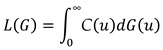
over the set of distribution functions $\Omega =\left\{G:G_1\left(u\right)\le G\left(u\right)\le G_2\left(u\right),u\ge 0\right\}$ and the integrand function satisfies conditions (*), then there exists a distribution function of the following structure among the distribution functions on which the maximum is achieved:

- or the function coincides with one of the boundaries;

- or the function moves from boundary to boundary;

- or a piecewise constant (stepped) function.

Proof of Theorem 1.

The proof of the theorem is carried out step by step: ordering of maxima, construction of reference functions, investigation of the properties of the reference functions and the proof of the theorem statement.

The ordering of the maxima is described above, so we will use the previously introduced notations.

Next, we describe the algorithm for constructing reference functions, determine their areas of values and definitions, and examine their structure and properties.

Note that the formulation of the theorem defines distribution functions that have structures of three kinds, which we will hereafter refer to as reference functions.

For each isolated global maximum of the integrand function $\left({\alpha }_1,u_{1j}\right),1\le j<k_1$ we define a reference function in the area $u\in \left[0,+\mathrm{\infty }\right]$

$$G_{1j}^{\mathrm{*}}\left(u\right)=\left\{\begin{array}{c}{G}_1\left(u_{1j}\right),u\in 0,u_{1j}\\ \mathit{min}\left(G_2\left(u_{1j}\right),G_1\left(u_{1j+1}\right)\right),u\in u_{1j},+\mathrm{\infty }.\end{array}\right..$$

(5)

Then we define the area of influence of each maximum by the ratio

$U^{\left(1,j\right)}=\left\{\begin{array}{c}{u}_{1j-1},u_{1j},еслиG_2^{\left(-1\right)}\left(G_1\left(u_{1j}\right)\right)\le u_{1j-1},\\ \left[u_{1j},u_{1j}\right],еслиG_2^{\left(-1\right)}\left(G_1\left(u_{1j}\right)\right)>u_{1j-1},u_{10}=0,\end{array}\right.$

and in the area of

$$U^{\left(1\right)}={\bigcup }_{1\le j\le k_1}{U}^{\left(1,j\right)}$$

(6)

let us construct a non-decreasing, stepped, continuous function on the left

$$G^{\mathrm{*}}\left(u\right)={\sum }_{j=1}^{k_1}\left(G_j^{\mathrm{*}}\left(u\right)-G_j^{\mathrm{*}}\left(0\right)\right),$$

(7)

satisfying the conditions

$$\begin{gathered} G_{1j}^{\mathrm{*}}\left(u_{1j}\right)=G_1\left(u_{1j}\right), \\ \underset{u\to u_{1j}+0}{lim}{G}_{1j}^{\mathrm{*}}\left(u\right)=\mathit{min}\left(G_2\left(u_{1j}\right),G_1\left(u_{1j+1`}\right)\right), \\ j=\mathrm{1,2},...,k_1. \end{gathered}$$

It is easy to see that function (7) coincides with the reference functions in the area (6).

Recall that if the global maximum of the ${\alpha }_1$ of the integrand function $\mathrm{С}\left(u\right)$ is reached on some segment $\left[u^{\left(1\right)},u^{\left(2\right)}\right]$then the maxima at the boundary points take part in the process of the maxima ordering. If for these maxima the inequality is satisfied

$$u^{\left(1\right)}<G_2^{\left(-1\right)}\left(G_1\left(u^{\left(2\right)}\right)\right),$$

then add to the set $U^{\left(1\right)}$ segment $\left[u^{\left(1\right)},G_2^{\left(-1\right)}\left(G_1\left(u^{\left(2\right)}\right)\right)\right]$ and define the reference function on this set as a stepped function having a finite number of jumps and belonging to the set of admissible functions.

Let us prove one important inequality, which is true for the reference function. To this end, we introduce the function

$$\tilde{A}\left(u\right)=\left\{\begin{array}{c}{\alpha }_1,u\in U^{\left(1\right)},\\ A\left(u\right),u\in U\left({\alpha }_1\right)\backslash U^{\left(1\right)}\end{array}\right.$$

For any admissible distribution $G\left(u\right)\in \Omega$ by virtue of the properties of the reference function $G^{\mathrm{*}}\left(u\right)$ and the major function $\tilde{A}\left(u\right)$ the following inequalities are true

$$\begin{gathered} {\int }_{U^{\left(1\right)}}A\left(u\right)dG\left(u\right)\le {\int }_{U^{\left(1\right)}}\tilde{A}\left(u\right)dG\left(u\right)\le \\ \le {\int }_{U^{\left(1\right)}}\tilde{A}\left(u\right)d{G}^{\mathrm{*}}\left(u\right)={\int }_{U^{\left(1\right)}}A\left(u\right)d{G}^{\mathrm{*}}\left(u\right) \end{gathered}$$

(8)

In addition to this property of the reference functions, we note another interesting inequality for the reference function and for any function $G\in \Omega$. Let us denote by ${\gamma }_{1j}=G_{1j}^{\mathrm{*}}\left(0\right),{\gamma }_{2j}=G_{1j}^{\mathrm{*}}\left(+\mathrm{\infty }\right)$ and define the function

$$G_{1j}\left(u\right)=\left\{\begin{array}{c}{\gamma }_{1j},u\in 0,G_{ }^{\left(-1\right)}\left({\gamma }_{1j}\right),\\ G\left(u\right),u\in G_{ }^{\left(-1\right)}\left({\gamma }_{1j}\right),G_{ }^{\left(-1\right)}\left({\gamma }_{2j}\right),\\ {\gamma }_{2j},u\in G_{ }^{\left(-1\right)}\left({\gamma }_{2j}\right),+\mathrm{\infty }.\end{array}\right.$$

(9)

From the definition of the reference functions and functions $G_{1j}\left(u\right)$ it follows the fulfillment of the inequalities

$$L\left(G_{1j}^{\mathrm{*}}\right)\ge L\left(G_{1j}\right).$$

(10)

If $U^{\left(1\right)}=U\left({\alpha }_1\right)$, the theorem is proved, since

$$L\left(G\right)=\sum _{j=1}^{k_1}L\left(G_{1j}\right)\le \sum _{j=1}^{k_1}L\left(G_{1j}^{\mathrm{*}}\right)=L\left(G_1^{\mathrm{*}}\right).$$

(11)

and among the optimal distributions there is a stepped function

$$G_1^{\mathrm{*}}\left(u\right)=\sum _{j=1}^{k_1}\left(G_{1j}^{\mathrm{*}}\left(u\right)-G_{1j}^{\mathrm{*}}\left(0\right)\right)$$

with jumps at the points of maxima.

If $U^{\left(1\right)}\subset U\left({\alpha }_1\right)$then $U_1=\left(U\left({\alpha }_1\right)\backslash U^{\left(1\right)}\right)\ne \mathrm{\varnothing }$ and set the problem to determine the reference function in this area. Note that this area is a finite number of intervals, in each of which, at least at one boundary point, the integrand function equals ${\alpha }_1$. Let us describe the process of determining the reference functions of one of them by denoting this interval $\left[u^{\left(1\right)},u^{\left(2\right)}\right]$. Then two variants are possible:

There are no maxima within the interval;

Within the interval there are maxima and a global maximum of the level $s,2\le s\le n$i.e. there are interior points $u_{sj},1\le l_1\le j\le l_2\le k_s$for which the equality is true $C\left(u_{sj}\right)={\alpha }_s$.

In the first case, the reference function in the area $\left[u^{\left(1\right)},u^{\left(2\right)}\right]$ we define by equality

$$G_{10}^{\mathrm{*}}\left(u\right)=\left\{\begin{array}{c}{G}_2\left(u^{\left(1\right)}\right),u\in 0,u^{\left(1\right)},\\ G_2\left(u\right),u\in u^{\left(1\right)},G_2^{\left(-1\right)}\left({\gamma }_{ }^{\mathrm{*}}\right),\\ {\gamma }_{ }^{\mathrm{*}},u\in G_2^{\left(-1\right)}\left({\gamma }_{ }^{\mathrm{*}}\right),G_1^{\left(-1\right)}\left({\gamma }_{ }^{\mathrm{*}}\right),\\ G_1\left(u\right),u\in G_1^{\left(-1\right)}\left({\gamma }_{ }^{\mathrm{*}}\right),u^{\left(2\right)},\\ G_1\left(u^{\left(2\right)}\right),u\in u^{\left(2\right)},+\mathrm{\infty }\end{array}\right..$$

(12)

where ${\gamma }_{ }^{\mathrm{*}}\in \left[G_2\left(u^{\left(1\right)}\right),G_1\left(u^{\left(2\right)}\right)\right]$ and for it the equality is done

$$\begin{gathered} \underset{\gamma \in \left[G_2\left(u^{\left(1\right)}\right)G_1\left(u^{\left(2\right)}\right)\right]}{max}\left({\int }_{u\in u^{\left(1\right)},G_2^{\left(-1\right)}\left(\gamma \right)}C\left(u\right)d{G}_2\left(u\right)+{\int }_{u\in G_1^{\left(-1\right)}\left(\gamma \right),u^{\left(2\right)}}C\left(u\right)d{G}_1\left(u\right)\right)= \\ =\left({\int }_{u\in u^{\left(1\right)},G_2^{\left(-1\right)}\left({\gamma }_{ }^{\mathrm{*}}\right)}C\left(u\right)d{G}_2\left(u\right)+{\int }_{u\in G_1^{\left(-1\right)}\left({\gamma }_{ }^{\mathrm{*}}\right),u^{\left(2\right)}}C\left(u\right)d{G}_1\left(u\right)\right)={\int }_{u\in u^{\left(1\right)},u^{\left(2\right)}}C\left(u\right)d{G}_{10}^{\mathrm{*}}\left(u\right) \end{gathered}$$

If there are no maxima inside the area $\left[u^{\left(1\right)},u^{\left(2\right)}\right]$, then there exists a point $u^{\left(0\right)}\in \left[u^{\left(1\right)},u^{\left(2\right)}\right]$for which $G_1\left(u^{\left(0\right)}\right)\le G_2\left(u^{\left(0\right)}\right)$ and in the area $\left[u^{\left(1\right)},u^{\left(0\right)}\right]$the integrand function does not increase, and in the area $\left[u^{\left(0\right)},u^{\left(2\right)}\right]$ the integrand function does not decrease. Let us introduce two functions

$$G_{10}\left(u\right)=\left\{\begin{array}{c}{\gamma }_1,u\in 0,G_{ }^{\left(-1\right)}\left({\gamma }_1\right),\\ G\left(u\right),u\in G_{ }^{\left(-1\right)}\left({\gamma }_1\right),G_{ }^{\left(-1\right)}\left({\gamma }_2\right),\\ {\gamma }_2,u\in G_{ }^{\left(-1\right)}\left({\gamma }_2\right),+\mathrm{\infty },\end{array}\right.$$

(13)

$${\Psi }_{10}^{\mathrm{*}}\left(u\right)=\left\{\begin{array}{c}{\gamma }_1,u\in 0,u^{\left(1\right)},\\ G_2\left(u\right),u\in u^{\left(1\right)},G_2^{\left(-1\right)}\left(G\left(u_{ }^{\left(0\right)}\right)\right),\\ G\left(u_{ }^{\left(0\right)}\right),u\in G_2^{\left(-1\right)}\left(G\left(u_{ }^{\left(0\right)}\right)\right),G_1^{\left(-1\right)}\left(G\left(u_{ }^{\left(0\right)}\right)\right),\\ G_1\left(u\right),u\in G_1^{\left(-1\right)}\left(G\left(u_{ }^{\left(0\right)}\right)\right),u^{\left(2\right)},\\ {\gamma }_{2}u\in u^{\left(2\right)},+\mathrm{\infty }.\end{array}\right.$$

From the definition of these functions at $G\in \Omega$ these inequalities follow

${\Psi }_{10}^{\mathrm{*}}\left(u\right)\ge G_{j0}\left(u\right),\mathrm{}\mathrm{}u\in 0,u^{\left(0\right)},$

${\Psi }_{10}^{\mathrm{*}}\left(u\right)\le G_{j0}\left(u\right),\mathrm{}\mathrm{}u\in u^{\left(0\right)},+\mathrm{\infty }.$If we consider the properties of the integrand function, it is easy to obtain an estimate by integrating over the parts

$${\int }_0^{+\mathrm{\infty }}C\left(u\right)d\left({\Psi }_{10}\left(u\right)-G_{10}\left(u\right)\right)\ge 0$$

From this evaluation and the choice of the parameter ${\gamma }_{ }^{\mathrm{*}}$ follows

$${\int }_{G_{ }^{\left(-1\right)}\left({\gamma }_1\right)}^{G_{ }^{\left(-1\right)}\left({\gamma }_2\right)}C\left(u\right)dG\left(u\right)={\int }_0^{+\mathrm{\infty }}C\left(u\right)d{G}_{10}\left(u\right)\le {\int }_0^{+\mathrm{\infty }}C\left(u\right)d{\Psi }_{10}\left(u\right)\le {\int }_0^{+\mathrm{\infty }}C\left(u\right)d{G}_{10}^{\mathrm{*}}\left(u\right)$$

(14)

This completes the construction of the reference functions for the interval in question.

Next, let us consider the case where there are maxima within the interval and the global maximum of the level $s,2\le s\le n$i.e. there are interior points $u_{sj},1\le l_1\le j\le l_2\le k_s$for which the equality $C\left(u_{sj}\right)={\alpha }_s$is true. Formally, it is necessary to reorder the maxima for the new area. We will leave the previous notations in order to avoid unnecessary cumbersomeness.

Let's define the areas $\left[u^{\left(1\right)},u_{s1}\right],\mathrm{}\left[u_{s{k}_s},u^{\left(2\right)}\right]$.

In the first area, the integrand function does not increase and the inequalities are satisfied

$${\alpha }_1\ge C\left(u\right)\ge {\alpha }_s,$$

(15)

and in the second area the integrand function does not decrease and the same inequalities (15) are satisfied for it.

Note that if one of the areas does not fulfill the inequalities, it is not further involved in the consideration.

If ${\gamma }^{\left(1\right)}=G_2\left(u_{s1}\right)\ge G_1\left(u_{s{k}_s}\right)={\gamma }^{\left(2\right)}$, then we define the reference function in $\left[{\gamma }^{\left(2\right)},{\gamma }^{\left(1\right)}\right]$ by the equality (12), where the parameter ${\gamma }_{ }^{\mathrm{*}}$ is defined by the relation

$$\begin{gathered} \underset{\gamma \in \left[{\gamma }^{\left(2\right)},{\gamma }^{\left(1\right)}\right]}{max}\left({\int }_{u\in u^{\left(1\right)},G_2^{\left(-1\right)}\left(\gamma \right)}C\left(u\right)d{G}_2\left(u\right)+{\int }_{u\in G_1^{\left(-1\right)}\left(\gamma \right),u^{\left(2\right)}}C\left(u\right)d{G}_1\left(u\right)\right)= \\ =\left({\int }_{u\in u^{\left(1\right)},G_2^{\left(-1\right)}\left({\gamma }_{ }^{\mathrm{*}}\right)}C\left(u\right)d{G}_2\left(u\right)+{\int }_{u\in G_1^{\left(-1\right)}\left({\gamma }_{ }^{\mathrm{*}}\right),u^{\left(2\right)}}C\left(u\right)d{G}_1\left(u\right)\right) \\ ={\int }_{u\in u^{\left(1\right)},u^{\left(2\right)}}C\left(u\right)d{G}_{10}^{\mathrm{*}}\left(u\right) \end{gathered}$$

Next, prove the inequality

$${\int }_{G_{ }^{\left(-1\right)}\left({\gamma }_1\right)}^{G_{ }^{\left(-1\right)}\left({\gamma }_2\right)}C\left(u\right)dG\left(u\right)\le {\int }_0^{+\mathrm{\infty }}C\left(u\right)d{G}_{10}^{\mathrm{*}}\left(u\right).$$

(16)

for any admissible distribution. The proof of this inequality is reduced to the introduction of a major function

$$\tilde{C}\left(u\right)=\left\{\begin{array}{c}{\alpha }_s,u\in \left[u_{s1},u_{s{k}_s}\right],\\ C\left(u\right),u\notin \left[u_{s1},u_{s{k}_s}\right]\end{array}\right.$$

and the definition of functions $G_{10}\left(u\right),{\Psi }_{10}^{\mathrm{*}}\left(u\right)$, only as a parameter $u^{\left(0\right)}$ can be any point of the area $\left[u_{s1},u_{s{k}_s}\right]$.

Finally, if ${\gamma }^{\left(1\right)}=G_2\left(u_{s1}\right)<G_1\left(u_{s{k}_s}\right)={\gamma }^{\left(2\right)}$, then we define two reference functions

$$G_{10}^{\left(1\mathrm{*}\right)}\left(u\right)=\left\{\begin{array}{c}{\gamma }_1,u\in 0,u_{ }^{\left(1\right)},\\ G_2\left(u\right),u\in u_{ }^{\left(1\right)},u_{s1},\\ {\gamma }_{ }^{\left(1\right)},u\in u_{s1},+\mathrm{\infty },\end{array}\right.$$

(17)

$$G_{10}^{\left(2\mathrm{*}\right)}\left(u\right)=\left\{\begin{array}{c}{\gamma }_{ }^{\left(2\right)},u\in 0,u_{s{k}_s},\\ G_1\left(u\right),u\in u_{s{k}_s},u_{ }^{\left(2\right)},\\ {\gamma }_2,u\in u_{ }^{\left(2\right)},+\mathrm{\infty },\end{array}\right.$$

(18)

and two functions associated with one admissible distribution function $G\in \Omega$,

$$\begin{gathered} G_{10}^{\left(1\right)}\left(u\right)=\left\{\begin{array}{c}{\gamma }_1,u\in 0,G_{ }^{\left(-1\right)}\left({\gamma }_1\right),\\ G\left(u\right),u\in G_{ }^{\left(-1\right)}\left({\gamma }_1\right),G_{ }^{\left(-1\right)}\left({\gamma }_{ }^{\left(1\right)}\right),\\ {\gamma }_{ }^{\left(1\right)},u\in G_{ }^{\left(-1\right)}\left({\gamma }_{ }^{\left(1\right)}\right),+\mathrm{\infty },\end{array}\right. \\ {G}_{10}^{\left(2\right)}\left(u\right)=\left\{\begin{array}{c}{\gamma }_{ }^{\left(2\right)},u\in 0,G_{ }^{\left(-1\right)}\left({\gamma }_{ }^{\left(2\right)}\right),\\ G\left(u\right),u\in G_{ }^{\left(-1\right)}\left({\gamma }_{ }^{\left(2\right)}\right),G_{ }^{\left(-1\right)}\left({\gamma }_2\right),\\ {\gamma }_2,u\in G_{ }^{\left(-1\right)}\left({\gamma }_2\right),+\mathrm{\infty }.\end{array}\right. \end{gathered}$$

Then two inequalities can be easily proved by integration over parts

$${\int }_{G_{ }^{\left(-1\right)}\left({\gamma }_1\right)}^{G_{ }^{\left(-1\right)}\left({\gamma }_{ }^{\left(1\right)}\right)}C\left(u\right)dG\left(u\right)={\int }_0^{+\mathrm{\infty }}C\left(u\right)d{G}_{10}^{\left(1\right)}\left(u\right)\le {\int }_0^{+\mathrm{\infty }}C\left(u\right)d{G}_{10}^{\left(1\mathrm{*}\right)}\left(u\right)$$

(19)

$${\int }_{G_{ }^{\left(-1\right)}\left({\gamma }_{ }^{\left(2\right)}\right)}^{G_{ }^{\left(-1\right)}\left({\gamma }_2\right)}C\left(u\right)dG\left(u\right)={\int }_0^{+\mathrm{\infty }}C\left(u\right)d{G}_{10}^{\left(2\right)}\left(u\right)\le {\int }_0^{+\mathrm{\infty }}C\left(u\right)d{G}_{10}^{\left(2\mathrm{*}\right)}\left(u\right).$$

(20)

It is easy to see that the reference functions in the area$u\in \left[u_{s1},u_{s{k}_s}\right]$are not defined. This procedure repeats the above, only for a new narrower area and a smaller maximum.

The procedure for constructing the reference functions will end due to the finiteness of the number of maxima of the integrand function.

So, a finite set of reference functions is constructed, which fields of values do not overlap and which sum coincides with $\left[\mathrm{0,1}\right]$. Denote by M the set of reference functions and define the function

$$G^{\left(0\right)}\left(u\right)=\sum _{G_{ }^{\mathrm{*}}\in \mathrm{М}}\left(G_{ }^{\mathrm{*}}\left(u\right)-G_{ }^{\mathrm{*}}\left(0\right)\right).$$

(21)

Since inequalities (11), (14), (16), (19), (20) for the reference functions are satisfied for any function $G\in \Omega$ we have the inequality

$$L\left(G\right)\le L\left(G^{\left(0\right)}\right)$$

which proves the statement of the theorem. □

3. Discussion

Let us formulate useful corollaries of the proved theorem.

Given the statement of the above lemma, we give a formulation for the fractionally linear functional (1), assuming the existence of a maximum of this functional $\underset{G\in \Omega }{max}I\left(G\right)=I\left(G_{ }^{\mathrm{*}}\right)=\mathrm{С}$ and fulfillment of the conditions of the theorem on the integrand functions.

Source 1

[4,5]. If $\Omega =\left\{G:G\left(u_i\right)={\pi }_i,0\le i\le n,0=u_0<u_1<...<u_n<u_{n+1}=+\mathrm{\infty },0={\pi }_9\le {\pi }_1\le ...\le {\pi }_n\le {\pi }_{n+1i}\right\}$, then

$$\underset{G\in \Omega }{max}I\left(G\right)=\underset{\begin{array}{c}{x}_k\in \left.u_k,u_{k+1}\right),\\ 1\le k\le n\end{array}}{max}\frac{{\sum }_{k=0}^{n}A\left(x_k\right)\left({\pi }_{k+1}-{\pi }_k\right)}{{\sum }_{k=0}^{n}B\left(x_k\right)\left({\pi }_{k+1}-{\pi }_k\right)}$$

Source 2

[6]. If the function $\mathrm{С}\left(u\right)=\mathrm{А}\left(u\right)-\mathrm{С}B\left(u\right)$ has one maximum at $\left[0,+\mathrm{\infty }\right]$, then

$$\underset{G\in \Omega }{max}I\left(G\right)=\underset{x\ge 0}{max}\frac{{\int }_0^{x}A\left(u\right)d{G}_1\left(u\right)+A{\left(x\right)}_1\left(G_2\left(x\right)-G_1\left(x\right)\right)+{\int }_x^{+\mathrm{\infty }}A\left(u\right)d{G}_2\left(u\right)}{{\int }_0^{x}B\left(u\right)d{G}_1\left(u\right)+B{\left(x\right)}_1\left(G_2\left(x\right)-G_1\left(x\right)\right)+{\int }_x^{+\mathrm{\infty }}B\left(u\right)d{G}_2\left(u\right)}$$

(22)

Source 3.

If the function $\mathrm{С}\left(u\right)=\mathrm{А}\left(u\right)-\mathrm{С}B\left(u\right)$ has no maxima in $\left(0,+\mathrm{\infty }\right)$, then

$$\underset{G\in \Omega }{max}I\left(G\right)=\underset{\gamma \in \left[\mathrm{0,1}\right]}{max}\frac{{\int }_{u\in 0,G_2^{\left(-1\right)}\left(\gamma \right)}\mathrm{А}\left(u\right)d{G}_2\left(u\right)+{\int }_{u\in G_1^{\left(-1\right)}\left(\gamma \right),+\mathrm{\infty }}\mathrm{А}\left(u\right)d{G}_1\left(u\right)}{{\int }_{u\in 0,G_2^{\left(-1\right)}\left(\gamma \right)}\mathrm{В}\left(u\right)d{G}_2\left(u\right)+{\int }_{u\in G_1^{\left(-1\right)}\left(\gamma \right),+\mathrm{\infty }}\mathrm{В}\left(u\right)d{G}_1\left(u\right)}$$

(23)

The following example of a controlled mass service model in the "classical" statement, when the constraints are formulated in the form of standard inequalities on probability measures $\Omega =\left\{G:0\le G\left(B\right)\le 1\right\}$ are well known [3], so we will omit the detailed conclusions of the basic relations.

Example 1. A mass service system.

We will study a mass service system, the input of which is a Poisson flow of demands with the parameter $\lambda$ comes. The number of service channels is one, the number of waiting places is $K,1\le K<\mathrm{\infty }$. In Kendall's terminology the system $\left(M\left|G\right|1|K\right)$.

In contrast to the classical formulation, we will change the distribution of the service time depending on the number of demands in the system at the moments of the end of service of the next demand and at the moments of arrival of demands to the free system. If at the given moments the number of demands in the system is equal to i, then we choose the service time distribution of the next demand equal to $G(i,t)=P\left\{{\xi }_i<t\right\}$where ${\xi }_i$ - is random service time. Assigning a random service duration means introducing randomization into the decision making process (a Markov moment), i.e. at the moment when a decision has to be made and state i is observed, the realization of $\tau$ of a random variable ${\xi }_i=\tau$ distributed according to the law $G\left(i,t\right)=P\left\{{\xi }_i<t\right\}$and the service duration is assigned equal to the value $\tau$.

Let's introduce the cost characteristics, which determine the functional that characterizes the quality of functioning and control.

Let:

$c_0$ - fee (income) per one serviced claim;

$c_1$ - payment for one hour of channel operation;

$c_2$ - payment for one hour of free channel idle time,

$c_3$ - payment for the loss of one claim,

$c_4$ - payment for one hour of one requirement in the queue.

In [3] there is an expression of fractionally linear functional (1) - the specific mathematical expectation of accumulated income for an arbitrary number of places for expectation $K,1\le K<\mathrm{\infty }$. We consider the solution of the above optimization problem under $K=\mathrm{1,2}$ and the constraints

$$0\le G_1(i,i,t)\le G(i,t)\le G_2(i,t)\le 1,$$

(24)

where $G_1(i,i,t),G_2(i,i,t),G_{11}\left(t\right)\le G_{21}\left(t\right)$ are the distribution functions belonging to the set $\Omega$.

With one waiting place $\left(K=1\right)$ at Markov moments (moments of end of service and moments of arrival of demands to the free system) there are either zero demands or one demand in the system.

Hence, a semi-Markov process has two states, but decisions are made only in one of them when there is one requirement in the system and the functional (1) depends on one distribution function $G(1,t)=G\left(t\right)$.

In [3] the dependence of this functional on the initial characteristics is given

$$I\left(G\right)=\frac{{\int }_0^{+\mathrm{\infty }}\left[\lambda \left(c_0+c_{1}t\right)+c_2{e}^{-\lambda t}+\left(\lambda t+e^{-\lambda t}-1\right)\left(c_3\lambda +c_4\right)\right]dG\left(t\right)}{{\int }_0^{+\mathrm{\infty }}\left(\lambda t+e^{-\lambda t}\right)dG\left(t\right)}.$$

(25)

Next, we will use the notation

$$A\left(t\right)=\lambda \left(c_0+c_{1}t\right)+c_2{e}^{-\lambda t}+\left(\lambda t+e^{-\lambda t}-1\right)\left(c_3\lambda +c_4\right),B\left(t\right)=\lambda t+e^{-\lambda t}.$$

Next, let us set the optimization problem: let there be two distribution functions

$$G_1(1,t),G_2(1,t),G_1(1,t)\le G_2(1,t),G_i\left(\mathrm{1,0}\right)=0,i=\mathrm{1,2}$$

(26)

and we need to find the maximum of the functional (25) over the set of distributions

$$\Omega =\left\{0\le G_1(1,t)\le G\left(t\right)\le G_2(1,t)\le 1\right\}.$$

By the conditions of the theorem and lemma proved above, it is necessary to investigate the function

$$C\left(t\right)=A\left(t\right)-CB\left(t\right)=\lambda \left(c_0+c_{1}t\right)+c_2{e}^{-\lambda t}+\left(\lambda t+e^{-\lambda t}-1\right)\left(c_3\lambda +c_4\right)-C\left(\lambda t+e^{-\lambda t}\right),$$

(27)

where $\underset{G\in \Omega }{max}I\left(G\right)=C$.

Let us investigate the function $C\left(t\right)$ and prove that it satisfies the conditions of the above theorem and has one maximum.

Suppose that the inequality $C>0$ is true for optimal demand service since the initial data should be such that, under optimal control, the operation of the mass service system should produce a positive effect.

It is important to pay attention to the sign of the initial constants. The coefficients $c_i,i=\mathrm{1,2},\mathrm{3,4}$ are negative, since they are losses from the functioning of the system; the parameter $c_0$ is greater than zero, because it is a profit.

The function under study (27) and all its derivatives are continuous.

The elementary ratios below

$$\begin{gathered} C\left(0\right)=\lambda c_0-C\ge 0,C\left(t\right)\to -\mathrm{\infty },t\to +\mathrm{\infty }, \\ \frac{dC\left(t\right)}{dt}=\lambda \left(\left(c_1+c_3\lambda +c_4-C\right)-\left(c_3\lambda +c_4+c_2-C\right)e^{-\lambda t}\right), \\ \frac{dC\left(0\right)}{dt}=\lambda \left(c_1-c_2\right),\frac{d^{2}C\left(t\right)}{d{t}^2}=\left(c_2+c_3\lambda +c_4-C\right){\lambda }^2{e}^{-\lambda t}\le 0, \end{gathered}$$

prove that this function has a maximum at some point $0\le t_0<+\mathrm{\infty }$and in the area $\left(0,t_0\right)$ it increases, and in the area $\left(t_0,+\mathrm{\infty }\right)$ it decreases. Thus, it is proved that the function $C\left(t\right)$ has a maximum at some finite point. Therefore the maximum of the functional (25) is reached on the function

$$G_{ }^{\mathrm{*}}\left(t\right)=\left\{\begin{array}{c}{G}_1(1,t){,}^{ }0\le t\le {\tau }_0,\\ G_2(1,t){,}^{ }{\tau }_0<t\le +\infty ,\end{array}\right.$$

the parameter ${\tau }_0$ is defined as the maximum point of the function

$$\begin{gathered} \underset{G_1\left(x\right)\le G\left(x\right)\le G_2\left(x\right)}{max}I\left(G\right)=\underset{0\le \tau \le +\mathrm{\infty }}{max}\frac{{\int }_0^{\tau }A\left(t\right)d{G}_1(1,t)+A\left(\tau \right)\left(G_2(1,\tau )-G_1(1,\tau )\right)+{\int }_{\tau }^{+\mathrm{\infty }}A\left(t\right)d{G}_2(1,t)}{{\int }_0^{\tau }B\left(t\right)d{G}_1(1,t)+B\left(\tau \right)\left(G_2(1,\tau )-G_1(1,\tau )\right)+{\int }_{\tau }^{+\mathrm{\infty }}B\left(t\right)d{G}_2(1,t)}= \\ =\frac{{\int }_0^{{\tau }_0}A\left(t\right)d{G}_1(1,t)+A\left({\tau }_0\right)\left(G_2(1,{\tau }_0)-G_1(1,{\tau }_0)\right)+{\int }_{{\tau }_0}^{+\mathrm{\infty }}A\left(t\right)d{G}_2(1,t)}{{\int }_0^{{\tau }_0}B\left(t\right)d{G}_1(1,t)+B\left({\tau }_0\right)\left(G_2(1,{\tau }_0)-G_1(1,{\tau }_0)\right)+{\int }_{{\tau }_0}^{+\mathrm{\infty }}B\left(t\right)d{G}_2(1,t)}, \end{gathered}$$

and the functions $A\left(t\right)$ and $B\left(t\right)$ are defined by the equations

$$\begin{gathered} A\left(t\right)=\lambda \left(c_0+c_{1}t\right)+c_2{e}^{-\lambda t}+\left(\lambda t+e^{-\lambda t}-1\right)\left(c_3\lambda +c_4\right), \\ B\left(t\right)=\lambda t+e^{-\lambda t}. \end{gathered}$$

Let us note the obvious conclusion: at $c_2\ge c_1$ we have $G_{ }^{\mathrm{*}}\left(t\right)=G_2(1,t)$.

Example 2. Reliability model.

Let a system be defined in which the time of no-failure operation $\xi$ is distributed according to the law $F\left(x\right)=P\{\xi <x\},\bar{F}\left(x\right)=P\left\{\xi x\right\}$. Suppose that a failure that occurs during the functioning of the system is independently detected (manifested) instantly.

At the initial moment t0=0 the system operation begins and the scheduled preventive update (preventive maintenance) of the system is assigned in time η≥ 0, distributed according to the law $G\left(x\right)=P\{\eta <x\},G\left(0\right)=0.$ The appointment of scheduled preventive updates of the system at random time means introduction of randomization in the decision making process, i.e. at the moment when decision should be made, the realization of τ random variable η ( =ητ ), distributed according to the law $G\left(x\right)$, and a scheduled preventive update of the system is performed after the time τ .

If the system has not failed by the appointed time η (the event {η <ξ } has occurred), then at the time η a planned preventive update of the system is started, which by assumption completely updates the system. Let us denote the duration of this scheduled preventive (prophylactic) update by ${\gamma }_1$, and $F_1\left(x\right)=P\{{\gamma }_1<x\}$ is a function of the distribution of this duration, ${\bar{F}}_1\left(x\right)=P\{{\gamma }_1\ge x\}$.

If the system has failed by the appointed time η , an unscheduled emergency update of the system begins at the time of the failure ξ . We denote the duration of this recovery operation by ${\gamma }_2$, and denote the distribution law by $F_2\left(x\right)=P\{{\gamma }_2<x\},{\bar{F}}_2\left(x\right)=P\{{\gamma }_2\ge x\}.$After possible remedial work, when the system is assumed to be completely renewed, the next precautionary remedial work is rescheduled and the entire maintenance process is repeated all over again.

Let us introduce a random process ξ (t), characterizing the state of the system at an arbitrary point in time t, by putting

ξ(t)=e0 if at time t the system is working properly;

ξ(t)=e1, if at time t the system undergoes a scheduled preventive update of the system;

ξ(t)=e3 if at time t an unscheduled emergency update of the system is performed.

The steady-state availability factor $K_{\mathrm{г}}$ is defined as the probability of catching the system in an operable state at an infinitely distant moment of time. In [7], this characteristic in the notations adopted above is defined by equality

$$K_{\mathrm{г}}\left(G\right)=\frac{{\int }_0^{+\mathrm{\infty }}{\int }_0^u\bar{F}\left(y\right)dydG\left(u\right)}{{\int }_0^{+\mathrm{\infty }}\left[{\int }_0^u\bar{F}\left(y\right)dy+M{\gamma }_1\bar{F}\left(u\right)+M{\gamma }_{2}F\left(u\right)\right]dG\left(u\right)}$$

The mathematical problem is to determine the distribution $G^{\mathrm{*}}\in \mathsf{\Omega }$for which

$$\underset{G\in \mathsf{\Omega }}{max}{K}_{\mathrm{г}}\left(G\right)=K_{\mathrm{г}}\left(G^{\mathrm{*}}\right)=C$$

Let us investigate the function

$$\mathrm{С}\left(u\right)=\left(1-C\right){\int }_0^u\bar{F}\left(y\right)dy-C\left[M{\gamma }_1\bar{F}\left(u\right)+M{\gamma }_{2}F\left(u\right)\right]$$

and obtain for the derivative the equality

$$\begin{gathered} \frac{d\mathrm{С}\left(u\right)}{du}=\left(1-C\right)\bar{F}\left(u\right)-C\left[M{\gamma }_2-M{\gamma }_1\right]f\left(u\right)= \\ =\bar{F}\left(u\right)\left[\left(1-C\right))-C\left(M{\gamma }_2-M{\gamma }_1\right)\lambda \left(u\right)\right], \end{gathered}$$

where it is marked $\lambda \left(u\right)=\frac{f\left(u\right)}{\bar{F}\left(u\right)},f\left(u\right)=\frac{dF\left(u\right)}{du}$Under the natural conditions $0\le C\le 1,M{\gamma }_2\ge M{\gamma }_1$ and the assumption that the system is aging, that is, the function $\lambda \left(u\right)$ is increasing, we obtain: the derivative changes sign from plus to minus no more than once.

Then

$$\begin{gathered} \underset{G\in \mathsf{\Omega }}{max}{K}_{\mathrm{г}}\left(G\right)=\underset{\tau \ge 0}{max}\frac{{\int }_0^{\tau }{\int }_0^u\bar{F}\left(y\right)dyd{G}_1\left(u\right)+{\int }_0^{\tau }\bar{F}\left(y\right)dy\left(G_2\left(\tau \right)-G_1\left(\tau \right)\right)+{\int }_{\tau }^{+\mathrm{\infty }}{\int }_0^u\bar{F}\left(y\right)dyd{G}_1\left(u\right)}{{\int }_0^{\tau }B\left(u\right)d{G}_1\left(u\right)+B\left(\tau \right)\left(G_2\left(\tau \right)-G_1\left(\tau \right)\right)+{\int }_{\tau }^{+\mathrm{\infty }}B\left(u\right)d{G}_1\left(u\right)}= \\ =\frac{{\int }_0^{{\tau }_0}{\int }_0^u\bar{F}\left(y\right)dyd{G}_1\left(u\right)+{\int }_0^{{\tau }_0}\bar{F}\left(y\right)dy\left(G_2\left({\tau }_0\right)-G_1\left({\tau }_0\right)\right)+{\int }_{{\tau }_0}^{+\mathrm{\infty }}{\int }_0^u\bar{F}\left(y\right)dyd{G}_1\left(u\right)}{{\int }_0^{{\tau }_0}B\left(u\right)d{G}_1\left(u\right)+B\left({\tau }_0\right)\left(G_2\left({\tau }_0\right)-G_1\left({\tau }_0\right)\right)+{\int }_{{\tau }_0}^{+\mathrm{\infty }}B\left(u\right)d{G}_1\left(u\right)} \end{gathered}$$

where $B\left(u\right)={\int }_0^u\bar{F}\left(y\right)dy+\left[M{\gamma }_1\bar{F}\left(u\right)+M{\gamma }_{2}F\left(u\right)\right]$.

Thus, the distribution is set

$$G^{\mathrm{*}}\left(u\right)=\left\{\begin{array}{c}{G}_1\left(u\right),0\le u\le {\tau }_0,\\ G_2\left(u\right),{\tau }_0<u\le +\infty ,\end{array}\right.$$

at which the maximum of the investigated functional is reached.

References

- Kashtanov, V. A. The Structure of the Functional of Accumulation Defined on a Trajectory of Semi-Markov Process with a Finite Set of States Theory of Probability & Its Applications 2016 60:2, 281-294. [CrossRef]
- Kashtanov, V. A. "Discrete Distributions In Control Problems". Probabilistic Methods in Discrete Mathematics: Proceedings of the Fourth International Petrozavodsk Conference, Petrozavodsk, Russia, June 3-7, 1996, edited by, Berlin, Boston: De Gruyter, 1997, pp. 267-274. 3 June. [CrossRef]
- Kashtanov V. A., Zaitseva O. B. Research of operations (linear programming and stochastic models). Textbook. Course, INFRA-M, Moscow, 2016. – 256 p.
- Barzilovich E. Yu. Yu., Kashtanov V. A., Kovalenko I. N. On minimax criteria in reliability problems. - "Proceedings of the Academy of Sciences of the USSR. Ser. of Technical Cybernetics", 1971, No.3, pp. 87-98.
- Barzilovich E. Yu., Kashtanov V. A. Organization of Service with Limited Information about System Reliability. - M. "Sovetskoe Radio", 1975. – 135 p.
- Kashtanov, V.A., Zaitseva, O.B. & Efremov, A.A. Controlled Semi-Markov Processes with Constraints on Control Strategies and Construction of Optimal Strategies in Reliability and Safety Models. Math Notes 109, 585-592 (2021). [CrossRef]
- Kashtanov V.A., Medvedev A.I. Reliability Theory of Complex Systems. Moscow: Fizmatlit, 2010. – 608 p.
Disclaimer/Publisher’s Note: The statements, opinions and data contained in all publications are solely those of the individual author(s) and contributor(s) and not of MDPI and/or the editor(s). MDPI and/or the editor(s) disclaim responsibility for any injury to people or property resulting from any ideas, methods, instructions or products referred to in the content. |
© 2023 by the authors. Licensee MDPI, Basel, Switzerland. This article is an open access article distributed under the terms and conditions of the Creative Commons Attribution (CC BY) license (http://creativecommons.org/licenses/by/4.0/).
Copyright: This open access article is published under a Creative Commons CC BY 4.0 license, which permit the free download, distribution, and reuse, provided that the author and preprint are cited in any reuse.