Submitted:
08 June 2023
Posted:
09 June 2023
Read the latest preprint version here
Abstract
The security of several full homomorphic encryption (FHE) schemes depends on the hardness of the approximate common divisor (ACD) problem. The analysis of attack and defense against the system is one of the frontiers of cryptography research. In this paper, the performance of existing algorithms, including orthogonal lattice, simultaneous diophantine approximation, multivariate polynomial and sample pre-processing are reviewed and analyzed for solving the ACD problem. Orthogonal lattice (OL) algorithms are divided into two categories (OL-$\land$ and OL-$\vee$) for the first time. And an improved algorithm of OL-$\vee$ is presented to solve the GACD problem. This new algorithm works well in polynomial time if the parameter satisfies certain conditions. Compared with Ding and Tao's OL algorithm, the lattice reduction algorithm is used only once, and when the error vector $\mathbf{r}$ is recovered in Ding et al.'s OL algorithm, the possible difference between the restored and the true value of $p$ is given. It is helpful to expand the scope of OL attacks.
Keywords:
Approximate common divisors
; Fully homomorphic encryption
; lattice attack
; orthogonal lattice
1. Introduction
It is well known that the Greatest Common Divisor (GCD) problem has been widely and deeply studied. Euclid algorithm is a classical algorithm for solving the GCD problem, which is called by Knuth [4] as the ancestor of all GCD algorithms. In the last two decades, many improvements to the GCD algorithms have been proposed. And these algorithms have a wide range of applications in computational algebra and cryptography. However, the approximate common divisor (ACD) problem remains a number theory problem. The ACD problem was first studied by Howgrave-Graham [5]. Further interest in this problem was proposed by the homomorphic encryption (FHE) scheme of Van Dijk et al. [16] and its variants [19,24,34]. The security of these cryptosystems depends on the hardness assumption of the ACD problem and its variants.
Fix , let p be an -bit odd integer, define the efficiently sampleable distribution as
The ACD problem is usually formulated in two ways: general approximate common divisor (GACD) problem and partial approximate common divisor (PACD) problem. Given polynomially many samples from for all i), to calculate p, which is the GACD problem. Given polynomially many samples from , as well as a sample for uniformly chosen , to compute p, which is the PACD problem.
By definition, PACD cannot be harder than GACD, and intuitively it seems that it should be easier than GACD. However, Van Dijk et al. ] mentioned that there was no PACD algorithm that did not work for GACD. And the usefulness of PACD was demonstrated by the construction [19], where a much more efficient variant of the scheme [16] was built, whose security relied on PACD rather than GACD. Thus, it is very important to get whether or not PACD is actually easier than GACD. Moreover, ACD problems were divided into computational and decision versions. Coron et al. [32] pointed out that the two versions are equivalent. By definition, PACD cannot be harder than GACD, and intuitively it seems that it should be easier than GACD. However, Van Dijk et al. [16] mentioned that there was no PACD algorithm that did not work for GACD. And the usefulness of PACD was demonstrated by the construction [19], where a much more efficient variant of the scheme [16] was built, whose security relied on PACD rather than GACD. Thus, it is very important to get whether or not PACD is actually easier than GACD. Moreover, ACD problems were divided into computational and decision versions. Coron et al. [32] pointed out that the two versions are equivalent.
The variant problems based on ACD mainly include CRT-ACD and CS-ACD. Cheon et al. [26] and Lepoint [33] call the problem of computing from the public key the CRT-ACD problem. Cheon and Stehle [34] proposed a FHE scheme whose parameters are set to , Where d is the depth of the circuit for homomorphism computation. The problem corresponding to this set of parameters is called CS-ACD. Despite the utility of the two variants, the algorithms that secures its security foundation have not been probed well enough.
The original papers [5,16] presented a few possible lattice attacks on this problem, including orthogonal lattices (OL), simultaneous diophantine approximation (SDA) and multivariate polynomial equations (MP). Further cryptanalytic work was done by [23,24,25,30,31,36,37,41,42,43,44]. This paper surveys and compares the known lattice algorithms for the ACD problem.
Our main contribution is to propose an improved algorithm of OL-∨ to reduce both space and time costs for solving the GACD problem. Another contribution is to give the possible difference between the restored and the true value of p when is recovered, which is helpful to expand the scope of OL attacks. Our third contribution is to analyze the application range and performance of SDA, OL, MP algorithms and pre-processing. These work is very helpful for cryptographic algorithm attacks to achieve better results.
2. Preliminaries
Throughout this paper, capital boldface letters denote matrices, e.g. , lowercase bold letters denote vectors e.g. . Let , be the inner product and the Euclidean length respectively. denote the transpose of matrix . The notation log refers to the base-2 logarithm. And denotes the largest integer not more than real number r.
2.1. Lattice
Definition 1
(Lattice). A rank-t lattice in the is spanned by t linearly independent vectors
where is a basis for and
is the corresponding basis matrix. The rank or dimension and determinant of are respectively denoted as and
If is a square matrix, then
In addition, when a set of column vectors is given, the orthogonal lattice is defined as }.
When , the lattice is called a full rank lattice. In fact, it is only necessary to consider the full rank lattice in Euclidean space. Therefore, the lattices mentioned below are full rank lattice.
The length of the shortest non-zero vector, denoted by , is a very important parameter of a lattice. It is expressed as the radius of the smallest zero-centered ball containing a non-zero linearly independent lattice vector. Generally, successive minima was defined as follows:
Definition 2
(Successive minima). Let be a lattice of rank t. For , the i-th successive minima is defined as
where is a ball centered at the origin.
For the shortest vector of a random lattice, the Gaussian hypothesis is expressed as follows:
Gaussian Heuristic (First Minima). Let be a full rank lattice in , then the length of the shortest non-zero vector in is estimated by
2.2. Lattice basis reduction
Lattice reduction algorithm is employed to transform a lattice basis to another basis, and the latter one is nearly orthongral with each other and relatively shorter. As far, the LLL algorithm [1] and the BKZ algorithm [17] are well-known lattice reduction algorithms.
Definition 3
(Gram Schmidt Orthogonalization). Given a sequence of t linearly independent vectors , the Gram Schmidt orthogonalization is the sequence of vectors defined by
where
Definition 4
(LLL reduction basis). Given a lattice basis , the corresponding Gram-Schmidt basis , is a reduced basis if and only if the following two conditions are satisfied:
- ①
- (Size condition) , for all ;
- ②
- (Lovász condition) , for all , where .
Definition 5
(Geometric Series Assumption[8],GSA). Given Gram-Schmidt basis ,
for , where is called GSA constant.
The Geometric Series Assumption (GSA) means the length of Gram-Schmidt basis with LLL reduction decays geometrically with quotient and indicates for .
In the subsections 3.1 and 3.2, the analysis based on the following assumptions:
Assumption 1 ([37]). Let be a “random” lattice of rank t and be an LLL-reduced basis for , then
and
Nguyen and Stehlé [9] have studied the performance of LLL on “random” lattices and have hypothesised that an LLL-reduced basis satisfies the improved bound (2). By analogy with the relationship between the worst-case bounds and , it is natural to suppose that (3) is hold.
Assumption 2([37]). Let be a “random” lattice of rank t and let be an LLL-reduced basis for , then
Nguyen and Stehlé [9] show that almost always in Figure 4, and certainly with overwhelming probability. Galbraith et al. make the heuristic assumption that for all , so it is easy to show that, for all , . So it leads to Assumption 2 for “random” lattices.
In the subsection 3.2.2, the conclusion of the following theorem will be used.
Theorem 1.
[29] Given a LLL reduction lattice basis , is the corresponding Gram-schmidt basis. The following results were hold:
- (1)
- ;
- (2)
- , for ;
- (3)
- , for ;
where , δ is the parameter in the Definition 4.
After the LLL algorithm, a number of lattice reduction algorithms emerged. In practice, the Block-Korkine-Zolotarev (BKZ) algorithm proposed by Schnorr and Euchner [3] has a good performance. For the BKZ algorithm, according to [17], the block size determines how short the output vector is. With the increase of , the output basis becomes much reduced but the cost significantly increases. Gama and Nguyen [12] identified the Hermite factor of the reduced basis as the dominant parameter in the runtime of the lattice reduction and the quality of the reduced basis. For an t-dimensional lattice , the Hermite factor
where is the first reduced basis vector of and is called as the root-Hermite factor. Chen [27] gave an expression between the root-Hermite factor and the block size :
Under the GSA and based on the Hermit factor (5), Xu et al. [42] gave an upper bound on the i-th reduced basis vector
3. Algorithms to solve ACD problem
In this section, the first three subsections describe and analysis the lattice-based algorithms (SDA, OL, MP) to solve the ACD problem, and the last subsection analyzes the prospects of the pre-processing technology for ACD samples, when sufficiently many samples are available.
3.1. Simultaneous Diophantine approximation (SDA)
Van Dijk et al. [16] showed that the ACD problem can be solved using the SDA method. The basic idea of this attack is to note that if for , where is small, then
for , where . That’s what it means the fractions are an instance of simultaneous diophantine approximation to . Once is determined, can be computed from
Hence,
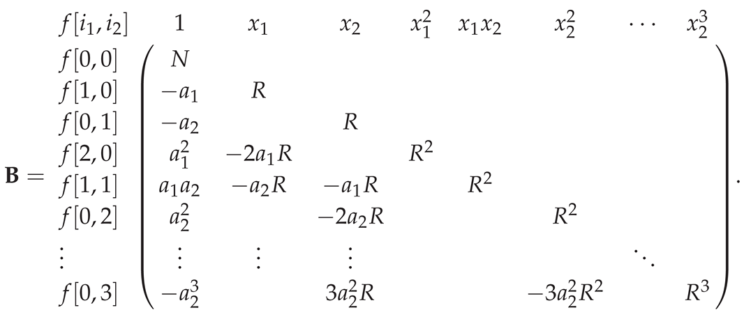
In fact, this attack does not benefit significantly from having an exact sample , so such a sample can be unknown. As in [16], construct the lattice of rank , which is generated by the basis matrix , where
Let , then
Since , the length of the first entry of is approximately . The length of the rest of entries of , which are of the form for , is estimated to be Therefore, is approximately
The vector satisfying the above conditions is called the target vector.
Hence, if
then the target vector is expected to be the shortest non-zero vector in the lattice. The attack is to run a lattice basis reduction algorithm to get a candidate for the shortest non-zero vector. The first entry of divided by will give a candidate for , then computes and . Finally test this value for p by checking if are small for all . This is the SDA algorithm.
A better approximation of tager vector is given by Van Dijk et al. [16], and an exact approximation
is given by Galbraith et al. [37]. That is to say about twice the above approximation (taking ).
Galbraith et al. [37] applies the Gaussian heuristic and to estimate
Hence, the target vector is the shortest vector in the lattice and is found by LLL if the expression (1) of Gaussian Heuristic is less than when multiplied by the factor according to Equation (3). Namely,
Ignoring constants and the term (the term does not have any significant effect on the performance of the algorithm[37]) in the above equation (8), a necessary (not sufficient) condition for the algorithm to succeed is
So t should be greater than to ensure that the target vector will likely be the shorest vector in the lattice . This lower bound on t is more advantageous for the analysis of CS-ACD [34]. For CS-ACD, if is close to , which means that for smaller , the dimension of the Lattice grows rapidly. Concretely speaking, the parameters in CS-ACD are set to
where d is the circuit depth and is the security paremeter. Let’s say , set , and then . For these values, . Therefore, in order to prevent lattice attacks, this ratio needs to be large enough. These arguments reconfirm that the method in [34] can provide more efficient parameters for homomorphic encryption.
3.2. Orthogonal Lattice (OL) based approach
Nguyen and Stern ([6]) have demonstrated the usefulness of the orthogonal lattice in cryptanalysis, and this has been used in several ways to attack the ACD problem. The idea is to find that is orthogonal to both and . Since , is orthogonal to . The task is to find linearly independent vectors shorter than any vector in to recover , and therefore p.
Based on the idea of Nguyen and Stern, the current idea is to find linearly independent vectors only orthogonal to . The core steps of the current OL algorithm include the following two steps:
First, find linearly independent vectors orthogonal to , that is,
then establish and solve indefinite equations
where
Let the general solution of (11) be
Where is a particular solution of (11), is the basis vector of the solution space of the corresponding homogeneous system of linear equations, and is the integer parameter.
Second, find small positive integer solutions to (11). At present, the common way to find the small solutions is to construct the lattice with basis matrix
Next, LLL algorithm is employed to reduce the basis matrix , and the first output is expected to be the vector . However, at present, what can meet this expectation are experimental conditions, and there is still a lack of theory. Now, the existing OL methods orthogonal to are classified. According to the constructed lattice, they are divided into two categories. The first OL algorithm constructs lattice with basis matrix :
and its shape likes ∧, so it is called OL-∧ algorithm. This kind of algorithm can be referred to [GGM16,XSH18].
The second OL algorithm constructs lattice with basis matrix :
where N is a big integer with bits . Or construct a lattice with basis matrix is :
Both (15) and (16) are all shaped ∨, so they are called OL-∨ algorithm. This kind of algorithm can be referred to [30,31,41,42].
3.2.1. OL-∧ algorithm
This algorithm uses the lattice mentioned above, and the basis matrix is , then
where is the identity matrix of order t, and
Therefore,
(I) When =2
Let in order to find the condition that is orthogonal to (t dimension), it needs to be satisfied
so it forces the equation
to be true. In order to make the equation (18) be established, Galbraith et al. ([37]) gives the bounds of the short vectors in the lattice :
Next, to show that under condition (19), formulas (17) and (10) hold, the following proof is given. Let , then and for . Thus
Because (19) is true and , . Hence
To prove that (10) holds, suppose , so
this is a contradiction.
To analyse the method, Galbraith et al. [37] use Assumption 2. This shows that LLL algorithm can be used to find linearly independent vectors as long as
and as well
Hence, the condition for success is
Ignoring constants and the exponential approximation factor from the lattice reduction algorithm, Galbraith et al. [37] gives a lower bound on sample t:
Find vectors that satisfies the bound of the short vector by LLL algorithm, then the system of equations can be set up to solve, and then find .
(II) in the general case
Using the bound of (6), the condition that is orthogonal to is constructed. Specific measures are as follows([42]):
- ①
- Let , then
- ②
- Using BKZ- alogrithm, reduce the lattice matrix . Let be the i-th reduce basis of , Then
Thus
Let
then minimize . Xu et al. [42] offer the following conclusion: When
Using the minimum of , the tighter bound of was found:
where
As analyzed by Xu et al. [42],
therefore
In order to make , the right side of the upper bound has to be less than 1:
thus the condition
holds. The dominant calculation of OL attacks is the lattice reduction for finding linearly independent homogeneous equations on or . Based on the condition (21), it is expected that
Since , the attack can work when
According to (22), it is obtained that
which is equivalent
When , the above expression is optimized as
Also notice that when , , then the logarithm term on t of condition (22) can reduce to get the following condition:
Similarly, taking , the above condition is optimimized as
(III) Using the rounding technique, construct a deformed lattice
3.2.2. OL-∨ algorithm
This algorithm uses the lattice mentioned above with basis matrix or the lattice with basis matrix .
(I) When
Let
to find the condition that is orthogonal to ( dimension), it needs to be satisfied:
then it is to force the equation
To make the equation true, Ding et al. [30] and Yang et al. [41] gave the bounds of the short vectors of the lattice , they are shown in (28) and (29) respectively,
In order to show that under the condition (28) or (29), formulas (26) and (27) hold, the following proof is given. Here, only condition (29) is used to prove.
Let , and .
Thus
Since
Therefore, there is no modular N operation and .
Next, it is easy to obtain that and hold.
(II) When
Let
in order to find the condition that is orthogonal to (t dimension), it needs to be satisfied:
In order to make (30) true, Yu et al. [41] and Gebregiyorgis et al. [36] gave the bounds of the short vectors in the lattice and they were given by the following formulas respectively,
After analysis, (32) is tighter than (31). Similarly, it can be proved that (30) holds under the condition (31) or(32). So the equations and can also be obtained.
(III) , lower bound estimating for the number of samples t
Under the GSA, Yu et al. use LLL algorithm to get the upper bound of -th short vector , by Theorem 1:
Due to
the bound of t in [30] is optimized, and the optimization result is given as follows [41]:
Yu et al. also indicates the hypothesis in [36]
is too strong and unreasonable, and is too small, it should be increased by 10 or 20.
For OL algorithm in [31], where or N works equally, the idea of this algorithm can be classified as OL-∨, and it is equivalent to the case
just N is the same as length as x , so the algorithm is a little bit more conservative.
In [31], the lattices and were defined, their basis matrices were and :
Let , then
For the sake of , it is to force the equation is true. Find a vector , such that the corresponding vector is orthogonal to . The experiment in [31] gives the following conditions that LLL algorithm can generate vectors (theoretically not proved):
- condition 1: N is a large random integer with bits;
- condition 2: ;
- condition 3: ;
- condition 4: ;
- condition 5: .
Under the above conditions, the equation is true. So can be solved and p is recovered.
(IV) in general
Similar to the idea of OL-∧ when is in general, the condition for is found by [XSH18-3.2]. The conclusions are as follows: the optimal value of is
and the condition
holds. The specific steps are below ([42]):
- ①
- Let , Then
- ②
- Using BKZ- alogrithm, reduce the basic matrix . Let be the i-th reduce basis of , Then
Thus
A little bit of clarification here. When , then the formula
is true. In order to make , the formula
holds, then
For finding linearly independent vectors orthogonal to , the following condition
is established. Next, let
then minimize . When
Using the minimum of , the tighter bound of was found:
where
As analyzed by Xu et al. [42],
therefore
In order to make , the right side of the upper bound has to be less than 1:
thus the condition
holds. The dominant calculation of OL attacks is the lattice reduction for finding linearly independent homogeneous equations on or . Based on the condition (34), it is expected that
Since , the attack can work when
According to (35), It is obtained that
which is equivalent
When , the above expression is optimized as
Also notice that when , , then the logarithm term on t of condition (36) can reduce to get the following condition:
Similarly, taking , this condition is optimimized as
3.2.3. Recover or
(1) Recover by LLL algorithm
Let the general solution formula of (11) be
where is a particular solution of (11), are the basis vectors for the solution space of the corresponding homogeneous system of linear equations, and are the integer parameters.
Next, find small positive integer solutions to (11) to get . Constract the lattice with basis matrix
Let , then
where are integers. Obviously, when , (40) = (38). Reduce the lattice to :
To facilitate finding , consider the explicit vectors . It’s easy to deduce that only one of them is the solution to (11).
Let is the solution to (11), and if , then is probably equal to . With this in mind, Ding and Tao [31] found the conditions that the algorithm can work well (see 3.2.2). In addition, if , we find an interesting thing that the recovery value is only 1 or 2 different from the true value p in many cases of our experiment. And our experiments lead to the following general conclusions between p and :
Let then
where is the recovered value of p. So, if , using vector , can be restored. And since is bounded, p can be restored by .
In summary, one of the outputs generated by the LLL algorithm can be used to recover under the appropriate conditions.
(2) Recover
Let , which satisfies LLL, where , LLL are the lattice basis matrix and LLL reduced lattice basis matrix respectively, then is a unimodular matrix with . Constract the system
Because with probability , where is the function of Euler-Rieamann zeta, the probability that is very high. Therefore is the absolute value of the last column of and [42]. It can be known from OL algorithm, the first row vector of matrix can be generated by LLL algorithm, but the t-th row vector has to satisfy the following equation:
If (43) is considered in isolation, it is very possible for (43) to be established. But from the above analysis, it can be seen that the matrix is a transition matrix from a basis of a lattice to its reduced basis, and is a unimodular matrix. Furthermore, through our experiments, it is difficult to guarantee that the last row vector of satisfies the equation (43). So finding such a matrix is still an open question.
3.2.3. An improved algorithm of OL-∨
In this part, an improved algorithm of OL-∨ is proposed. Constract a lattice with the basis matrix
where N is an integer with bits. Using the lower bound of t in [41] and the upper bound of the short vector in [36], the following improved Algorithm 1 is given.
When
this algorithm can successfully recover p. It is an improvement of Ding and tao’s OL algorithm [31]. Firstly, the lower bound of t and the upper bound of the short vector are modified. Secondly, the later step using the LLL algorithm has been cancelled in the recovery of . This is because when the algorithm is implemented with isolve command of Maple, the special solution of the equations (11) is exactly the small positive integer solution under the condition (44). Thirdly, unlike Ding and tao’s OL algorithm [31] which is not proved theoretically, our algorithm is correct theoretically. And it can be seen that the attack range is extended greatly and the efficiency increases quickly.
| Algorithm 1 An improved OL algorithm for GACD |
|
Input: An appropriate positive integer and ACD samples . Output: Integer p. 1. Randomly choose . 2. Reduce lattice by LLL algorithm with . Let the reduced basis be , where 3. If , where , then solve the integer linear system with t unknowns as follows 4. . 5. Compute . Return p. |
3.3. Multivariate polynomial (MP) equations method
Howgrave-Graham ([5]) is the first to consider reducing the PACD problem by giving two ACD sample inputs, and . The idea is based on finding small roots of modular univariate linear equations of the form for unknown p. It is generalized to a multivariate version in [16] which is called MP method. In fact, MP method is an extension of Coppersmith’s method ([Cop96b]). A rigorous analysis of this algorithm was provided by Cohn and Heninger [25] and a variant for the case when the “errors” are not all the same size was given by Takayasu and Kunihiro [28]. It is well-known that MP approach has some advantages if the number of ACD samples is very small, but the application with a large number of samples in actual cryptanalysis needs a great deal of attention. In addition, the MP approach can be applied to both PACD and GACD problems, but it is simpler to explain and analyse the PACD problem. Hence, in the following discussion, only this case will be told.
Notice that some notations change here. let and let for be our ACD samples, where for some given bound R. The idea is to construct a polynomial in m variables such that for some k. The parameters m and k are to be optimized. In [25], such a multivariate polynomial is constructed as integer linear combinations of the products where l is chosen such that .
Let
Here, the bound of the polynomial degree t has to be chosen. It doesn’t do any good to talk about , because it leads to the entire matrix being multiplied by the scalar for the case . Accordingly, Cohn and Heninge [25] consider the lattice generated by the coefficient row vectors of (45) such that and . If the occurrence of monomial in is sorted in inverse lexicographical order, then the basis matrix for the lattice is lower triangular. For example, when , the corresponding basis matrix is :
It is shown that the dimension of the lattice is , and its determinant is
where , . The following is a brief proof of and .
Clearly, is the number of possible polynomials of the form
in the variables . So, count the possible number of combinations of the exponents , where , so that . Assigning values to m exponents can be denoted by . Equivalently, count the number of non-negative integer solutions to the equation in the variables . It has possible number of solutions. Note that since
and
Adding all possible number of solutions for gives the result
Next, , where is the sum of exponents of N and is the sum of exponents of R. Because there are in total monomials with of them having exponent i. This implies that R has exponent . Summing up for gives the total exponent of R. So
The exponent of N in each monomial expression is l, where A similar analysis gives the exponent of N to be
Substituting N and R by their size estimates and respectively gives the result
Let be a vecor in and
then
If , clearly the equation holds over the integers. So the norm of needs to be bounded. Notice that
where the norm represents the sum of the absolute values of the components for the vector . Hence, if for some k, then is the target vector found in the MP algorithm. In order to save time and memory, more than m algebraically independent target vectors are usually selected for elimination. By using Gröbner basis method or the existing corresponding results to reduce the system to a univariate polynomial equation and hence solve for . Then can be determined.
When , the MP algorithm is the same as the orthogonal lattice attack [DGHV10, CH13, GGM16]. Such parameters are called “unoptimised”. The question is whether the algorithm is better at .
3.3.1 The heuristic analysis results of the MP algorithm in [25]
Cohn and Heninger [25] give a heuristic theoretical analysis of the MP algorithm and suggest optimal parameter choices . Later, Galbraith et al. sketched CH approach in [37]. The main results of the analysis are presented here.
Result 1. Let , so that , then the parameters satisfy the relational expression
Proof. Because the MP algorithm is executed successfully, m vectors satisfying need to be generated. Using and the bounds from Assumption 2, the LLL-reduced basis satisfying the condition can be found, where d is the dimension of the lattice. If this bound is less than , then enough vectors are needed to be obtained. Hence,
and so
Let , so that . With the first two terms of (46) deleted and approximating , , the formula (46) can be reduced to
Result 2 (Heuristic). For fixed m, if and , then the ACD problem can be solved in polynomial time.
Remark 1.
Result 2 does not imply that the MP approch is better than the SDA or OL approches. When is small, all algorithms based on lattices of dimension approximately , and the lattice input size is proportional to, so they are all polynomial time if they return a correct solution to the problem.
3.3.2 The heuristic analysis results of the MP algorithm in [36]
Gebregiyorgis [36] solved the corresponding polynomial equations in m variables. The following conclusion was obtained.
Result 3. Under the hypothesis
where , is short if .
Proof. If , then which implies
So
which is implied by
This is equivalent to
For , the first m output vectors of the LLL algorithm satisfy giving us polynomial relations between . Let and consider the d monomials in degree reverse ordering. Then the corresponding polynomial to lattice vector is
Next, collect m such independent polynomial equations. The system of equations can be solved using the Gröbner basis algorithms to find . Note that the first m output of the LLL algorithm do not necessarily give an algebraic independent vectors. In this case, subsequent vectors generated by the LLL algorithm with norm less than (if there are any) need to be added. Alternatively, to get algebraic independent polynomial equations, the polynomial equations needs to be factored. Finally, p is recovered with a high probability by computing .
The drawback of the CH-approach is that enough independent polynomial equations cannot be discovered. Gebregiyorgis’s experiment shows that this is the case. Moreover, the running of the Gröbner basis part is stuck even for small parameters.
3.3.3. The heuristic analysis results of the MP algorithm in [37]
Galbraith et al. [37] analyzed the conclusions of [25] and considered the parameters more generally, where it was assumed that the optimal solution would be to take . Here are the main results.
Result 4. The condition in Result 2 means the MP attack can be avoided in practice relatively easily.
Remark 2.
The OL method does not have any such hard limit on its theoretical feasibility. However, in practice the restriction is not so different from the usual condition that the dimension must be at least . If , then the required dimension would be at least , which is infeasible for lattice reduction algorithms for the parameters used in practice.
Result 5. For CS-ACD parameters, Galbraith et al. [37] suppose (e.g., ) and for some , their experimental condition implies that in which case . So this bound suggested that MP approach has no advantage over other methods for parameters of CS-ACD. Their experimental results also confirm this.
Result 6. When m is large, the best choices for the MP algorithm are , and so MP method was not better than the SDA or OL methods by practical experiments.
3.4. Pre-processing of the ACD samples
The most important factor in the hardness of the ACD problem is the ratio , which is the size of the integers relative to the size of p. The main idea of pre-processing method is: for the same p, without changing the size of the errors , reduce and find an easier set of ACD instances.
The method of preserving the sample size was analysed briefly in [36] and further discussion about preserving and aggressive shortening the sample size was given in [37]. Here is a brief overview and the statistic analysis of Galbraith’s results [37] on the pre-processing method.
The main idea of the pre-processing is the step by taking differences for and . The essence is that if then but and are not affected at not. Hence, is an ACD sample for the same p but with a smaller q and a similar sized error r. It is natural to want to be able to iterate this process until the sample size is suitable for the OL attack.
3.4.1 Preserving the sample size
Let the original samples , and the samples at iteration k are of the form
so the error terms is a “random” sum of -bit integers:
Since the are uniformly distributed, for large k,
So the condition of is expected. The analysis results in [37] are as follows:
Result 7. An absolute upper limit on the number of iterations is , and after the final iteration, the samples are reduced to bitlength no fewer than bits.
Remark 3.
Let be the intial -bit ACD samples. Suppose , b is typically 8 or 16. After I iterations, approximately samples are generated, each of bits. If , then the errors have grown so large that all information about p is lost essentially. Hence, an absolute upper limit on the number of iterations is ). This means that after the final iteration the samples are reduced to bitlength no fewer than bits.
Result 8. The pre-processing approach can make very little effect on the ACD problem.
Remark 4.
An attack on the original ACD problem requires a lattice of dimension roughly (assuming ). After k iterations of pre-processing, a lattice of dimension was needed. Even in the best case when taking and keep the denominator constant at , the lattice dimension is lowered from to . Since or 16, the lattice dimension decreased very little.
3.4.2 Aggressive shortening
The idea of the aggressive shortening method in [37] is to generate new samples (that are still about the same bitlength) by taking sums/differences of the initial list of samples. The steps consist of the following four steps:
Step 1. Let be a set of ACD samples, with having mean and standard deviation given respectively by
Let
that is to say, the m random sums of l elements of were generated. So
Step 2. Sort the new samples to obtain the list . These are called order statistics and are represented by .
Step 3. Consider the neighbouring differences or spacings for , and derive the statistical distribution of the spacings.
Step 4. Store the spacings as input to the next iteration of the algorithm. After I iterations, OL attacks can be applied.
The following analysis results were presented in [37]:
Result 9. The total number of iterations performed satisfies .
The complexity is proportional to , since each iteration computes a sorted list of size m. The mean and the standard deviation of the spacings is inversely proportional to m, so m is expected to be very large. Suppose, at the j-th iteration, a list of values are (so ) with standard deviation . The statistical distribution of such generic spacings have Exponential distributions. Suppose are independent and identically distributed random variables on with common distribution function F, inverse distribution function and density function . If denote the order statistics of , then the k-th spacing is well-approximated for large m as an Exponential random variable with (rate) parameter [37]. In particular, Suppose are normally distributed with mean and variance , then , where and g are respectively the inverse distribution function and density function of a standard Normal random variable. Let denote the function , Galbraith et al. [37] have been graphed and analyzed that H is a moderately small value away from the extreme order statistics, for example for . Thus the spacings have an Exponential distribution (with parameter depending on k) given by with mean .
Remark 5.
As noted in [37] that a random sum is well-approximated as a Normal random variable with variance for . The k-th spacing in this Normal approximation case essentially has a distribution given by with mean . when , so by considering the “middle” spacings of , random variables can be obtained with approximately the same distribution that are in general independent. Thus at the end of the j-th iteration, random variables is obtained, with mean and standrad deviation . After j iterations, the random variables are sums of of the original ACD samples, so the standard deviation of an error term in the output of the j-th has increased by a multiple of . Hence, the total number of iterations performed satisfies .
Result 10. To have samples of size close to -bits thus required Optimistically taking , the number of new samples m should satisfy: In other words, m is close to .
Remark 6.
After i iterations, the average size of samples is .
Result 11. In practice, m was prohibitively large. For the parameter sizes required for a cryptographic system, the resulting errors grew too rapidly to be useful for the neighbouring difference.
4. Comparisons of OL with SDA and MP algorithms
The ACD problem is currently a hard problem for appropriate parameter settings. Some cryptographic applications exploited the hardness problem of ACD. The homomorphic encryption schemes over the integers are particular examples, such as [16,19,34,35,38]. The security analysis of these schemes was based on the complexity of different algorithms to analyze and solve the ACD calculation problem. These algorithms were in turn based on the worst-case performance of the lattice reduction algorithm. It is important to analyze the current most effective algorithm to solve the ACD problem from practical point of view.
4.1 Comparision with the SDA algorithm
The SDA-approach (see Section 3.1) solves the ACD problem using simultaneous diophantine approximation method. The dimension of the lattice required is greater than . As if the proportion of these parameters is too large, the LLL algorithm cannot produce the desired output.
Van Dijk et al. [16] and Galbraith etal. [36] point out that the SDA algorithm is comparable to the performance when in the OL-∧ approach. Hence, the OL-∧ attack using the rounding technique is the fastest since it employs the input basis matrix with smaller entries, especially when is small. This fact is confirmed by experiments of Xu et al. [42].
4.2. Comparison of the two types of OL attacks
At first, the following asymptotic complexity estimatioans are given. Then according to operating conditions that depend on , the corrsponding comparion is presented.
Theorem 2.
Theorem 3.
([42]) For given -ACD instances and some sufficiently large security parameter , if the condition
holds, then the time complexity for solving-ACD instances isby running BKZ-if one SVP oracle costs.
Comparision of the OL-∧ attacks According to the analysis in Section 4.1 of [42], OL-∧ attacks in Section 3.2.1, cases (II) and (III) have the same asymptotic time complexity. Notice that in OL-∧ attack, the entries of input basis matrix in case (III) are approximately reduced by bits compared to that in case (II). Hence, the OL-∧ attack in case (III) will be faster in practical cryptanalysis. In typical scenarios, the OL-∧ attack in case (III) only achieves a constant improvement of the overall attack complexity. Based on the time complexity in the paper [20], the acceleration caused by reducing the number of bits is . This improvement may be quite significant in practice.
Comparision with the two types of OL attacks When , all these OL attacks for solving the -ACD problem have the same asymptotic time complexities; the OL-∧ attack is more advantageous than the OL-∨ attack when is relatively small; the case (II) is almost close to the case (III) of OL-∧ attack.
In order to hinder the attack of OL-∧, for the security parameter of [16], the following are the asymptotics conditions given by various literature.
condition 1: ([16]);
condition 2: ([34]);
condition 3: ([42]).
Obviously, condition 2 is better than condition 1. Compared to the condition 2 in [34], condition 3 in [42] is better in the case that is relatively small.
Galbraith et al. [36] showed the success condition of the case (I) of OL-∧ attack based on the LLL algorithm. In [42], when is in general case, the two OL attacks based on the BKZ- algorithm, the expression on ACD parameters , the number t of ACD samples and the root-Hermite factor were given by (24). This expression can be used to evaluate the specific security of ACD-based schemes.
4.3. Comparision with the MP Algorithm
The common drawback of MP Algorithm is that the dimensions and entries of the involved lattices are quite large, which affects the speed of the algorithm. Galbraith et al.([36]) pointed out that the MP approach is not better than the OL-∧ attack for practical cryptanalysis. Hence, the OL-∧ attacks in case (II) and (III) have more advantageous than the MP approach.
4.4. Brief summary
Theorem 4.
([42])The time complexities to solve -ACD instances by running BKZ- if one SVP oracle costs is given:
- ①
- The OL-∧ with : ;
- ②
- The OL-∨ with : .
5. Cryptanalysis of OL attacks in ACD-based FHE Schemes
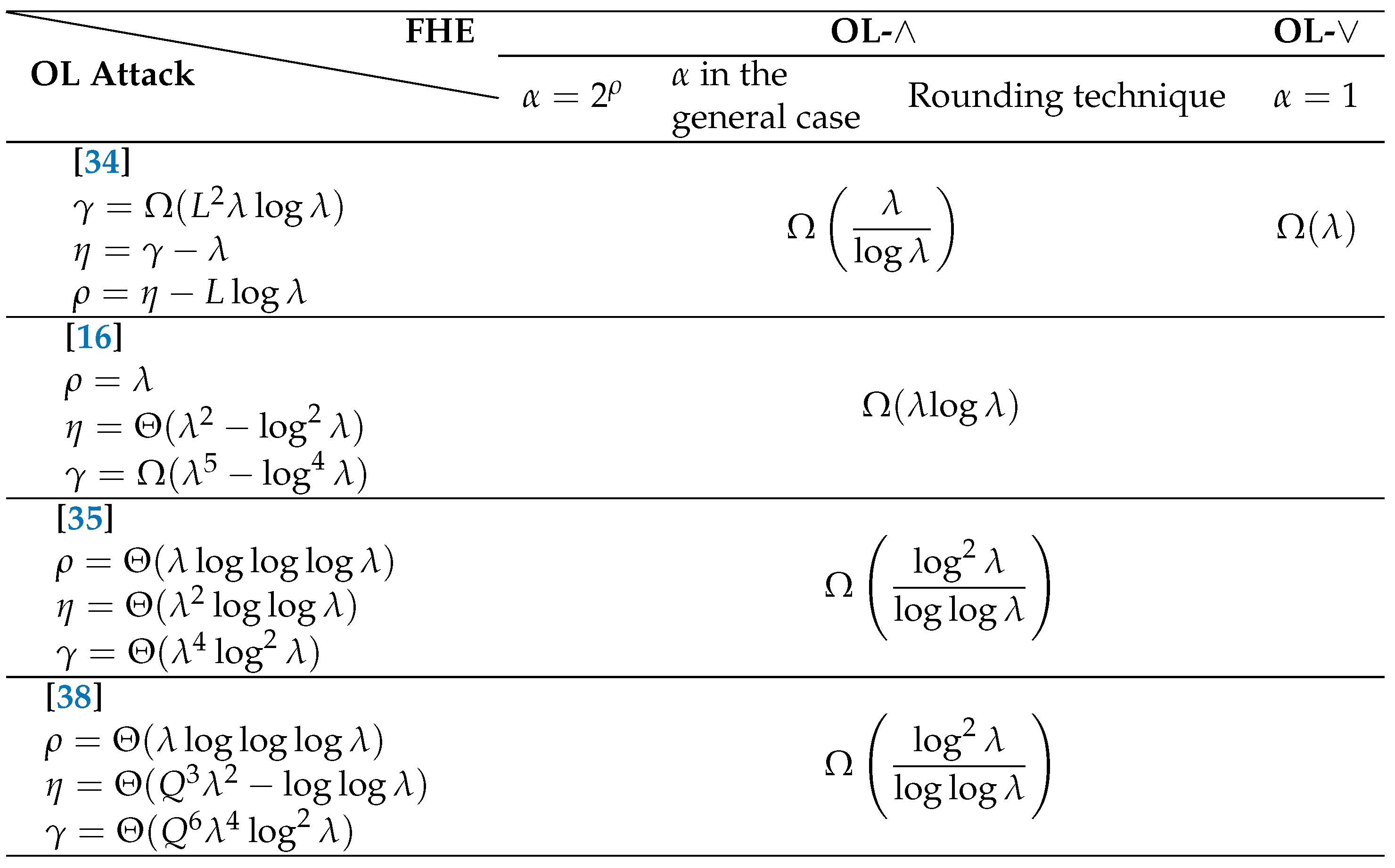
In this section, by using OL attack, the time complexity of the ACD problem in FHE scheme [DGHV10, KN15, CS15, KT16] is analysed and summarized. In particular, Cheon and Stehle [34] proposed a homomorphic encryption scheme whose parameters are
where d is the depth of the circuit for homomorphic calculation, here is no longer satisfied. They also indicated that if the (decision) ACD problem can be solved, then it can be solved LWE. And this set of parameters is obviously difficult.
According to Theorem 2 and Theorem 4, the log of the asymptotic time complexities for solving -ACD instances are summarized as Table 3.
Through the analysis of the Table 3, the following conclusions can be drawn:
①For the scheme of [16], those parameters are conservative to get -bit security for OL attacks. Further, according to Theorem 3, using instead of in order to achieve -bit security;
②For the scheme of [35], those parameters are optimistic to achieve -bit security for the OL attacks. Furthermore, based on 3, taking instead of for obtaining -bit security;
③For the scheme of [38], Q does not effect the asymptotic time complexities of OL attacks compared to the case of the [35] Scheme. The corresponding parameters are also optimistic to achieve -bit security for the OL attacks;
④For the scheme of [34], the asymptotic time complexities of obtainning the most significant bits of p for OL attacks is presented.
6. Prospects
Based on the above survey of ACD problem attacks , the ACD problem can be solved under certain conditions using the SDA, OL, MP algorithms. These results show that the applicable range of the three algorithms can be expanded even further. To date, several FHE schemes have been designed based on ACD and variant problems. Existing schemes conservatively set the parameters to be secure against these algorithms. Therefore, it is still worth further exploration to improve the existing algorithms for solving the ACD problem.
Although the present survey offers an initial contribution to the literature concerning the algorithms for ACD problem, the following open problems for further research are left. The application of the improved algorithm in section 3.2.3 needs to be considered for achieving cryptanalysis. Whether the algorithm can be improved to reduce parameter constraints.
For future work, our work points to some directions for addressing the ACD problem, which has great potential in term of further improvement in both theory and practice. This improvement is very much related to the Hermit factor of the reduction algorithm.
7. Conclusions
In this paper, known attacks on the ACD problem are investigated. The performance and application range of each algorithm are analyzed. OL algorithms are divided into two categories (OL-∧ and OL-∨) for the first time. This work is very helpful for OL attacks to achieve better results. An improved algorithm of OL-∨ is presented to solve the GACD problem. This algorithm works well in polynomial time if the parameter satisfies certain conditions. Compared with [31], the lattice reduction algorithm is used only once, and when the error term is recovered in [31], the possible difference between the restored and the true value of p is given. It is helpful to expand the scope of OL attacks.
Author Contributions
Conceptualization, Ran Y. and Wang L.; Methodology, Ran Y. and Wang L.; Validation, Pan Y. and Wang L.; Writing—original draft preparation, Ran Y.; Writing—review and editing, all; Code implementation, Ran Y. and Wang L.; Supervision and project administration, Pan Y.
Funding
This research is partially supported by the National Natural Science Foundation of China (NSFC) (62272040).
Conflicts of Interest
The authors declare no conflict of interest.
References
- A. K. Lenstra; H. W. Lenstra; and L. Lovász. Factoring polynomials with rational coeffcients. Math. Ann. 1982, 261(4): 515–534.
- J. C. Lagarias. The computational complexity of simultaneous Diophantine approximation problems. SIAM J. Comput. 1985, 14(1): 196–209. [CrossRef]
- Claus-Peter Schnorr and M. Euchner. Lattice basis reduction: Improved practical algorithms and solving subset sum problems. Math. Program. 1994, 66: 181–199. [CrossRef]
- D. E. Knuth. The art of computer programming, seminumerical algorithm[J]. Software: Practice and Experience, 1982, 12(9): 883–884.
- N. Howgrave-Graham. Approximate integer common divisors. Cryptography and Lattices. Springer Berlin Heidelberg, 2001: 51–66.
- P. Q. Nguyen and Jacques Stern. The Two Faces of Lattices in Cryptology. In J. Silverman (ed.), Cryptography and Lattices, Springer LNCS 2146, 2001: 146–180.
- Avrim Blum, Adam Kalai and Hal Wasserman. Noise-tolerant learning, the parity problem, and the statistical query model. Journal of ACM, 2003, 50(4): 506–519. [CrossRef]
- Claus-Peter Schnorr. Lattice reduction by random sampling and birthday methods. In STACS 2003, 20th Annual Symposium on Theoretical Aspects of Computer Science, Berlin, Germany, February 27–March 1, Proceedings, 2003: 145-156.
- Phong, Q. Nguyen and Damien Stehlé. LLL on the Average. In Florian Hess, Sebastian Pauli and Michael E. Pohst (eds.), ANTS-VII, Springer LNCS 4076, 2006: 238-256.
- V. Lyubashevsky. The Parity Problem in the Presence of Noise, Decoding Random Linear Codes, and the Subset Sum Problem. APPROX-RANDOM 2005, Springer LNCS 3624, 2005: 378–389.
- C. Gentry, C. Peikert, V. Vaikuntanathan. Trapdoors for hard lattices and new cryptographic constructions[C], Proceedings of the fortieth annual ACM symposium on Theory of computing. ACM, 2008: 197–206. [CrossRef]
- N. Gama and P. Q. Nguyen. Predicting lattice reduction. In Advances in Cryptology-EUROCRYPT 2008, 27th Annual International Conference on the Theory and Applications of Cryptographic Techniques, Istanbul, Turkey, April 13–17, 2008. Proceedings, 2008: 31-51.
- C. Gentry. A Fully Homomorphic Encryption Scheme. PhD thesis, The department of computer science, Stanford University, Stanford, CA, USA, 2009.
- P. Q. Nguyen, Valle B. The LLL algorithm: survey and applications. Springer Publishing Company, Incorporated, 2009.
- C. Gentry, Toward basing fully homomorphic encryption on worst-case hardness, in: T. Rabin(ed.), Advances in Cryptology-CRYPTO 2010, Lecture Notes in Comput. Sci. Springer, Berlin, Heidelberg, 2010, 6223: 116–137.
- M. Van Dijk, C.Gentry, S. Halevi, V. Vaikuntanathan, Fully homomorphic encryption over the integers, in: H. Gilbert (ed.), Advances in Cryptology—EUROCRYPT 2010, Lecture Notes in Comput. Sci. Springer, Berlin, Heidelberg, 2010, 6110: 24–43.
- G. Hanrot, X. Pujol, and D. Stehlé. Terminating bkz. IACR Cryptology ePrint Archive, 2011: 198.
- H. Cohn, N. Heninger. Approximate common divisors via lattices. CoRR, abs/1108. 2714, 2011.
- J. S. Coron, A. Mandal, D. Naccache, M. Tibouchi, Fully homomorphic encryption over the integers with shorter public keys, in: P. Rogaway (ed.), Advances in Cryptology-CRYPTO 2011, Lecture Notes in Comput. Sci, Springer, Berlin, Heidelberg, 2011, 6841: 487–504.
- A. Novocin, D. Stehlé, and G. Villard. An LLL-reduction algorithm with quasi-linear time complexity: extended abstract. In Proceedings of the 43rd ACM Symposium on Theory of Computing, 2011: 403–412.
- S. D. Galbraith, Mathematics of Public Key Cryptography. Cambridge University Press, 2012.
- Y. Ramaiah, G. Kumari, Efficient public key generation for homomorphic encryption over the integers[C]. Third International conference on advances in communication, network and computing. 2012.
- Y. Chen, P. Q. Nguyen. Faster algorithms for approximate common divisors: Breaking fully homomorphic encryption challenges over the integers. Advances in Cryptology-EUROCRYPT 2012. Springer Berlin Heidelberg, 2012: 502–519.
- J. S. Coron, D. Naccache, M. Tibouchi. Public Key Compression and Modulus Switching for Fully Homomorphic Encryption over the Integers. In D. Pointcheval and T. Johansson (ed.), EUROCRYPT’12, Springer LNCS, 2012, 7237: 446–464.
- H. Cohn, N. Heninger. Approximate common divisors via lattices. In proceedings of ANTS X, vol. 1 of The Open Book Series, 2013: 271–293.
- J. H. Cheon, J. S. Coron, J. Kim, M. S. Lee, T. Lepoint, M. Tibouchi, and A. Yun. Batch fully homomorphic encryption over the integers. In Proc. of EUROCRYPT, Springer LNCS, 2013, 7881: 315-335.
- Y. Chen. Réduction de réseau et sécurité concrète du chiffrement complètement homomorphe. Ph.d theses, Paris 7, June 2013.
- Atsushi Takayasu and Noboru Kunihiro, Better Lattice Constructions for Solving Multivariate Linear Equations Modulo Unknown Divisors, IEICE Transactions 97-A, 2014, 6: 1259-1272.
- J. Hoffstein, J. Pipher, and J. H. Silverman. An Introduction to Mathematical Cryptography. Springer Publishing Company, 2nd edition, 2014.
- J. Ding, C. Tao. A New Algorithm for Solving the General Approximate Common Divisors Problem and Cryptanalysis of the FHE Based on the GACD problem. Cryptology ePrint Archive, Report 2014/042, 2014.
- J. Ding, C. Tao. A New Algorithm for Solving the Approximate Common Divisor Problem and Cryptanalysis of the FHE based on GACD. IACR Cryptol. ePrint Arch, 2014: 42.
- J. S. Coron, T. Lepoint, M. Tibouchi, Scale-Invariant Fully Homomorphic Encryption Over the Integers, in: H. Krawczyk (ed.), Public-Key Cryptography—PKC 2014, Lecture Notes in Comput. Sci. Springer, Berlin, Heidelberg, 2014, 8383: 311-328.
- T. Lepoint. Design and Implementation of Lattice-Based Cryptography. Cryptography and Security [cs.CR]. Ecole Normale Supérieure de Paris-ENS Paris, 2014.
- J. H. Cheon, D. Stehlé. Fully Homomorphic Encryption over the Integers Revisited. In E. Oswald and M. Fischlin (eds.), EUROCRYPT’15, Springer LNCS, 2015, 9056: 513-536.
- K. Nuida, K. Kurosawa. (Batch) Fully Homomorphic Encryption over Integers for Non-Binary Message Spaces. Springer, Berlin, Heidelberg, 2015.
- S. Gebregiyorgis. Algorithms for the Elliptic Curve Discrete Logarithm Problem and the Approximate Common Divisor Problem. PhD thesis, The University of Auckland, Auckland, New Zealand, 2016.
- S. Galbraith, S. Gebregiyorgis, S. Murphy. Algorithms for the approximate common divisor problem. LMS Journal of Computation and Mathematics. 19(A), 2016.: 58-72. [CrossRef]
- Eunkyung Kim and Mehdi Tibouchi. FHE over the integers and modular arithmetic circuits. In Cryptology and Network Security-15th International Conference, CANS 2016, Milan, Italy, November 14-16, 2016, Proceedings, 2016: 435–450.
- D. Benarroch, Z. Brakerski, T. Lepoint. FHE over the Integers: Decomposed and Batched in the Post-Quantum Regime. Springer, Berlin, Heidelberg, 2017.
- J. Dyer, M. Dyer, J. Xu. Order-preserving encryption using approximate integer common divisors,Data Privacy Management, Cryptocurrencies and Blockchain Technology: ESORICS 2017 International Workshops, DPM 2017 and CBT 2017, Oslo, Norway, September 14-15, 2017, Proceedings. Springer International Publishing, 2017: 257–274.
- Xiaoling Yu, Yuntao Wang, Chungen Xu, Tsuyoshi Takagi. Studying the Bounds on Required Samples Numbers for Solving the General Approximate Common Divisors Problem. 2018 5th International Conference on Information Science and Control Engineering. [CrossRef]
- J. Xu, S. Sarkar, L. Hu, Revisiting orthogonal lattice attacks on approximate common divisor problems and their applications. Cryptology ePrint Archive, 2018.
- J. H. Cheon, W. Cho, M. Hhan, Algorithms for CRT-variant of approximate greatest common divisor problem. Journal of Mathematical Cryptology, 2020, 14(1): 397–413. [CrossRef]
- W. Cho, J. Kim, C. Lee. Extension of simultaneous Diophantine approximation algorithm for partial approximate common divisor variants. IET Information Security, 2021, 15(6): 417–427. [CrossRef]

Table 1.
Compare the effects of SDA, MP, CN and OL algorithms on ACD problem
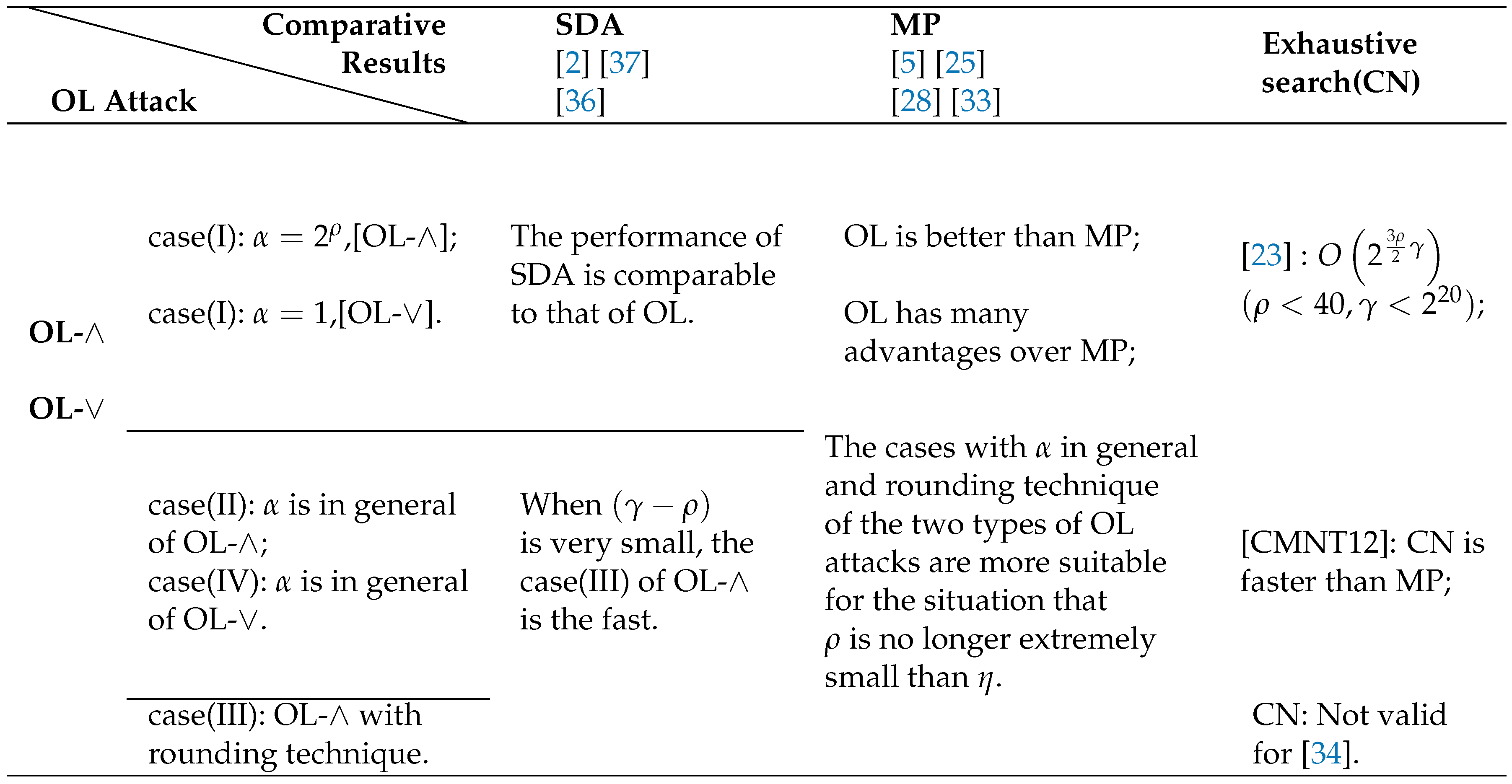
Table 2.
Comparison of Algorithms OL-∧ and OL-∨

Table 3.
Comparison of Algorithms OL-∧ and OL-∨
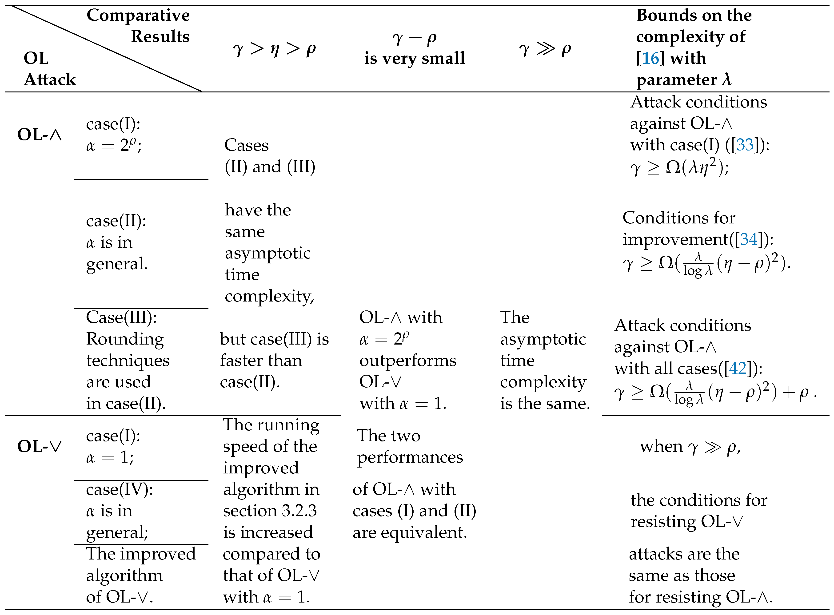
Table 4.
Cryptanalysis of FHE schemes based on ACD.
Disclaimer/Publisher’s Note: The statements, opinions and data contained in all publications are solely those of the individual author(s) and contributor(s) and not of MDPI and/or the editor(s). MDPI and/or the editor(s) disclaim responsibility for any injury to people or property resulting from any ideas, methods, instructions or products referred to in the content. |
© 2023 by the authors. Licensee MDPI, Basel, Switzerland. This article is an open access article distributed under the terms and conditions of the Creative Commons Attribution (CC BY) license (http://creativecommons.org/licenses/by/4.0/).
Copyright: This open access article is published under a Creative Commons CC BY 4.0 license, which permit the free download, distribution, and reuse, provided that the author and preprint are cited in any reuse.


