
Submitted:
08 June 2023
Posted:
08 June 2023
You are already at the latest version
Abstract
Crack inspection is important to monitor the structural health of pavement structures
and to facilitate an easier rehabilitation process. Currently, pavement crack inspection is conducted
manually, which is inefficient and costly at the same time. For solving the problem, this work has
developed a robotic system for automated data collection and analysis in real-time. The robotic
system navigates on the pavement and collects visual images from the surface. A deep learning-based
semantic segmentation framework named RCDNet was proposed and implemented on the onboard
computer of the robot to identify cracks from the visual images. Simulation results show that the deep
learning model obtained 96.29% accuracy for predicting the images. The proposed robotic system was
tested on both indoor and outdoor environments and was observed that it can complete inspecting a
3m × 2m grid within 10 minutes and a 2.5m × 1m grid within 6 minutes. This outcome shows that
the proposed robotic method can drastically reduce the time of manual inspection. Furthermore, a
severity map based on the results from visual images was also generated to provide an idea of which
locations should be paid more attention to repair in a test grid.
Keywords:
crack detection
; deep learning
; mobile robotic system
; NDE analysis
; pavement inspection
1. Introduction
Roads in South Korea are constituted by a length of 105673 KM of which 89,701 are paved roads (91.6%) [1]. These pavement roads can be damaged due to various reasons including surface cracking, delamination, honeycomb, etc. Cracks in pavement roads are one of the most potent indicators of pavement damage. Cracking in the pavement is quite unavoidable and there are many underlying factors (e.g., exposure to the sun, rain erosion, natural weathering, and long-term driving of the vehicle) that accelerate the pavement surface cracking. If these cracks cannot be localized and repaired in time, they will have a negative impact on the safe driving of vehicles. Consequently, it can cost deadly accidents as well as expenditure of a huge amount of money for the maintenance and repairment of pavements. So, crack detection at an early stage is very essential to inspect as well as evaluate the structural health and serviceability of the paved roads. Over the decades, manual crack detection was a very common practice for localizing cracks on paved roads. However, the manual method lacks efficiency and accuracy, it is expensive because of the involvement of the domain experts. Moreover, it is considerably tedious, arduous, and time-consuming because the experts monitor the cracks with the naked eye by roaming along the roads. Therefore, for lessening the workload of the experts and making the system fast as well as cost-effective, researchers are bringing automation the crack detection. With the advancement of Computer Vision (CV) technology, various vision-based methodologies have already been developed for performing automatic crack detection. Early implementation of the CV techniques for crack detection was to some extent limited to the threshold-based approaches (i.e. pixel intensity was used as the feature) [2,3], and other hand-crafted feature-based approaches. Some of the prominent hand-crafted feature extraction techniques are: wavelet features [4], Local Binary Pattern (LBP) [5], Digital Image Co-relation [6], Gabor filters [7], and so on. But these methods can only extract the local patterns instead of the global patterns which pulls the detection results backward. A few research works [8,9,10] used model-based traditional CV algorithms which use geometric characteristics of the images to perform crack detection in a global view. The advantages of the model-based techniques over the feature-based techniques are that the model-based techniques can detect cracks in adverse conditions such as noisy environments, poor illumination conditions, shadow problems, etc. Though these model-based methods can partially solve the noise problems and can detect cracks more continuously, their performance is not satisfactory enough during detecting cracks with complex patterns or intensity inhomogeneity.
In recent years, Deep Learning is being extensively applied in CV tasks for its noteworthy representation ability. DL models do not need hand-crafted features rather they can extract valuable features (both local and global) automatically from the input data. A few research works have already devoted their efforts to utilizing the properties mentioned above of deep learning for learning robust feature representation and detecting cracks with more precision. Zhang et al introduced Convolutional Neural Network (CNN) classifier for the first time in 2016 for detecting cracks in concrete structures [11]. The primary objective of this study was to develop a patch-based classifier for detecting cracks in concrete structures. Later on, Cha et al. [12], and Eisenbach et al. [13] also performed patch-based classification which can only identify the presence or absence of cracks in a corresponding image patch. Researchers also utilized another scheme of deep learning called object detection for localizing the cracks along with identification in an image [14,15]. However, these models can only classify and localize the cracks in a concrete structure instead of detecting cracks at a pixel level. So, for solving this issue, Yang et al. incorporated an image segmentation technique for detecting concrete cracks at a pixel level [16]. Crack segmentation involves classifying each of the pixels in an image as ’crack’ or ’non-crack’. Instead of predicting the class only in an image; crack segmentation predicts an output image highlighting the pixels containing the cracks which localize the cracks as well as extracts the original shape of the cracks. Moreover, the segmented images can later be used for finding out a few important pieces of information (i.e. crack length, width, area) which give ideas about crack severity in concrete structures. Considering the advantages of crack segmentation over crack detection and classification researchers from all over the world are devoting their efforts to developing crack segmentation methods and quantifying the cracks to present an automated crack detection system [17,18].
However, along with the automated detection of cracks, automatic data collection is also necessary for developing a fully automated pavement inspection system. While automated crack detection increases accuracy, automated data collection can save time and also handle safety issues. As a whole, many research works have already utilized robotic vehicles as well as unmanned aerial vehicles for collecting the images automatically [19,26]. However, most research works collect the data by their vehicle and transfer them to another computer for analysis, which can not be considered as e real-time detection for saving time. So, considering the above-mentioned issues, this work is going to develop a robotic-assisted pavement inspection system by which this work collects image data automatically as well as detects cracks from images in real time by using our proposed deep learning models. Furthermore, after predicting the images this work will quantify the cracks for presenting the severity maps of the cracks. In this work, this work will solve the problems of manual crack detection techniques through our proposed system. The automatic data collection will save time and also handle the safety issues, the detection using our proposed deep learning model will increase the accuracy, and finally, as this work is proposing a totally automated pavement inspection system, it will not need expertise involvement which will reduce the expenses also. This work is going to develop a robotic-assisted pavement inspection system. The main contributions of this study are:
- Developing a robotics platform that will collect visual data automatically.
- Presenting a novel deep learning model for implementing it on the robot onboard computer to detect cracks from the RGB images in real-time.
- Presenting a crack quantification algorithm for finding out crack length, width, and area.
- Finally, presenting a visualization of the crack severity map.
The rest of this research is organized as follows: Section 2 provides an overview of the existing research works which focus on developing robotic vehicles for pavement inspection. Section 3 presents the architecture of the robotic platform used in this work. Section 4 presents the crack segmentation technique from RGB images. Section 5 presents the working principle of the robotic platform. Section 6 discusses the experimental procedure and shows the obtained result of our proposed system. This work is concluded in Section 7.
2. Literature Review
In this Section, this work will briefly summarize the existing state-of-the-art related works which focus on developing robotic-assisted systems for inspecting cracks in concrete structures in real-time.
2.1. Robotic System for Crack Inspection
Over the past decades, various research works have been performed for developing robotic vehicles to inspect cracks automatically. The first work this study discusses in this section dated back to 2007 [19], designed an automated inspection system of cracks in concrete tunnels using a mobile robot. They collected the images by using a CCD camera which was interfaced with the robot and stored the images in the robot’s brain. Later the extracted cracks on a different computer using the Sobel edge detection algorithm. Like [19] Oyekola et al. also designed a robotic system for detecting cracks on concrete tank surfaces [20]. The authors also first collected the images and later detected cracks using a thresholding algorithm developed by the MATLAB programming language. Li et al. utilized the robotic platform developed by Guimu Robot Co Ltd. for detecting cracks on the pavement structures [21]. The authors developed an unsupervised algorithm named Multiscale Fusion Crack Detection (MFCD) for inspecting the cracks. However, in this work also the cracks are not detected in the onboard computer. La et al. developed a wall climbing robot for detecting cracks on steel bridges [22]. The robot was equipped with several sensors and a camera as well. During navigating through the steel bridges it collected data and passed them in real-time to the ground station for further processing and detecting cracks using a Hessian-matrix-based filter. In another work, La et al. used the Seekur mobile robot platform and modified it by installing several NDE sensors (e.g., GPR, USW, ER, IE), and a camera for concrete bridge deck monitoring [23]. The authors collected the images and passed them to the remote computer for extracting the cracks using a Gradient-based algorithm. They also presented the delamination maps of the cracking using the NDE data. The robot could localize itself and maneuver automatically on the bridge deck. However, this robotic system needs multiple onboard computers for navigating and processing everything. Hendrik et al. developed a legged robot named ANYmal for inspecting the crack conditions in the underground tunnels [24]. The authors considered the tactile sensory system instead of the vision data because of the presence of noise, water, etc. on the surface. They collected the signals from the footstep of the robot and classified the crack conditions using the Support Vector Machine (SVM) algorithm. The authors classified 5 types of crack conditions including good, satisfactory, fair, critical, and failure for providing an idea about the severity. Le et al. developed a mobile robotic system for in-line inspection of the pipes [25]. The authors integrated multiple sensors (e.g. Lidar, optic sensors) on the robot and classified these combined sensory data by the SVM algorithm for detecting cracks on the pipes. Lei et al. developed a low-cost unmanned aerial vehicle for inspecting cracks in concrete structures [26]. They collected the images using their UAV and classified cracks by the SVM classifier running on the onboard computer. Pan et al. utilized low-altitude images collected from UAV for detecting cracks on asphalt pavements [27]. The authors collected centimeter-level spatial resolution images and utilized a hybrid model (ANN+SVM) for inspecting the cracks. Montero et al. developed a mobile robotic system for detecting cracks in concrete tunnels [28]. They designed the mobile robot with a movable crane and a robotic arm. The movable crane carries the vision sensor and the robotic arm while the robotic arm carries an ultrasonic sensor. They designed the crane as movable so that it can reach different heights and directions for collecting data accurately. They collected images and passed them to the host computer which analyze the images using CNN and they contacted the ultrasonic sensor also with the tunnel wall for analyzing the cracks. Li et al. developed a quadrotor flying robot for detecting cracks in concrete bridges and tunnels [29]. The authors focused on reconstructing 3D metrics for knowing the location of the defects and severity information by a visual-inertial fusion approach. They proposed a novel Deep Learning model named AdaNet to detect cracks using their own crafted dataset named Concrete Structure spalling and Cracking (CSSC). Gui et al. developed a robotic system using the ARIR robotic platform for detecting cracks on airport pavement [30]. They utilized one vision camera and GPR sensor for collecting surface and subsurface data. The data were passed to an analysis center to process the collected data. They employed an intensity-based algorithm for detecting cracks from images and a voting-based CNN to predict the GPR data. Finally, the authors stitched the collected data to present a continuous grid for visualization. Ramalingam et al. developed a mobile robotic platform named Panthera for segmenting cracks and detecting garbage on the road [31]. The authors adopted SegNet for the segmenting task and a DCNN-based object detector for detecting garbage. Furthermore, they utilized Mobile Mapping System (MMS) for localizing the defects also. He et al. developed an unmanned surface vessel (USV) for inspecting cracks on the bottom part of bridges or urban culverts [32]. The authors installed both RGB cameras and LIDAR for collecting information from the environment. The authors proposed a novel Deep Learning model name CenWholeNet for detecting cracks. The USV was controlled from a ground station module where the LIDAR and video information was also transmitted from the robot’s brain (Intel NUc mini pc). Yang et al. developed a wall climbing robot for detecting cracks and spalling on concrete structures [33]. The authors collected data using an RGB-D camera and predicted the cracks on the images by utilizing a novel deep learning model named InspectionNet deployed in Intel Nuc Mini PC. They also developed a map-fusion module for their work to highlight the detected cracks. Yuan et al. developed a mobile robotic platform for detecting cracks in reinforced concrete structures [34]. The authors proposed a Mask-RCNN-based model for segmenting the cracks on the images collected from a stereo camera. They utilized an Nvidia Jetson Xavier device to implement the edge computing technique and pass the predicted frames to the host computer through the WebSocket protocol. They designed a UI for successfully controlling the robot and collecting the frames. Another important feature of this work is that after quantifying the damages the researchers presented actual size information on a 3D cloud point reconstruction of the inspected structures. Table 1 presents the summary of the robotic platforms for crack inspection. Though there is already much remarkable research works for detecting pavement cracks automatically, there is still a huge research scope for improving the methods. To the best of our knowledge, no previous works except [33,34] quantified the cracks after detecting them by their robotic system. Besides this, to the best of our knowledge, no previous works considered both indoor and outdoor environments for inspecting cracks by a robotic-assisted system. After considering the research scope, this work is going to develop a robotic-assisted maintenance system for pavement structures that will combine automated data acquisition, DL-based crack detection, crack quantification, and severity mapping in both indoor and outdoor environments.
3. Architecture of the AMSEL Robot
The design and configuration of the AMSEL robot developed for pavement crack inspection are described in this Section. Figure 1 displays the configuration in the lab environment and Table 2 presents the specifications of the robot.
3.1. Mechanical Unit
The mechanical system of the AMSEL robot is comprised of two different components; (a) a Chassis module unit, and (b) a Reconfigurable sensory frame. Figure 2 displays the mechanical components of the AMSEL platform.
3.1.1. Chassis module
The chassis module is the physical frame of the AMSEL robotic platform which give the vehicle a distinct shape. Figure 2a (i) and (ii) display the chassis of the AMSEL robot with and without the metal cover. The shape of the AMSEL chassis is a rectangle like a mobile robot. The chassis is made of lightweight steel. The dimension of the chassis is 21×48.5×71 centimeters. The motors, motor drivers, power source, and other electrical, as well as controller components, are accommodated on the left, and right rails and center of the chassis box. The box is covered with a metal plate, which carries the wifi router and keeps the components secure from rain and dust inside the chassis box.
3.1.2. Reconfigurable sensory frame
The sensor frame carries the vibration sensors, solenoids, and vision sensors. The sensor frame has a reconfiguration mechanism to go down for making contact between the vibration sensors and the ground as well as go up during the navigation time. Figure 2 b (iii) and (iv) shows the sensor frame in two different modes. The height, width, and length of the frames are 35, 36, and 17 centimeters respectively when the sensors are not touching the ground. The stepper motor is also attached to the frame for moving it up and down.
3.2. Electrical & Functional Unit
The electrical and programming unit of the AMSEL robot consists of three different types of components; (a) sensory units, (b) electrical units, and (c) control units. Figure 3 illustrates the electrical and sensory components.
3.2.1. Electrical Units
The AMSEL robot’s electrical block consists of various devices including a camera, battery, power supply board, DC motors, etc. The list and short description of the utilized electronic devices are provided below:
- Vision System: A Logitech c922 Pro HD Stream Webcam has been utilized as the vision system of the AMSEL robotic platform (Figure 3a (i)).
- Power source: In the AMSEL robot, a Polytronics Lithium-Polymer (Li-Po) battery has been used as the power source. The model number of the utilized battery is PT-B16-Fx30 (Figure 3a (ii)).
- Power supply board: A custom-designed power supply board has been utilized to split the power from the Li-Po battery among the other electronic devices used in the robotic platform (Figure 3a (iii)).
- DC motors: For navigating the robot, four DC motors have been used in the AMSEL robot (Figure 3a (iv)). The DC motors used in this robot are 200W Brushless DC (BLDC) motors. The model number of these motors is TM90-D0231.
- BLDC motor controller: For driving and controlling the motors in the AMSEL robot four BLDC motor controller have been used (Figure 3a (v)). The model number of the utilized controller is TMC-MD02.
- Serial communication adapter: The AMSEL robotic platform uses multiple serial communication adapters for converting the RS485 communication to USB communication as the system’s main controller uses USB communication protocol (Figure 3a (Vi)).
- Router A Tplink Archer Ax73 outer has been used in the AMSEL robot for communicating with the host pc in the ground station (Figure 3a (vii)).
3.2.2. Control Unit
The control system of the AMSEL robotic platform is divided into two parts mainly. One is the software control unit and the other one is the hardware control unit. For the software control, a graphical user interface (GUI) (Figure 4) has been designed using python programming language and implemented on a host computer at the ground station.
The GUI communicates with the primary hardware controller of the AMSEL robot using socket communication technology, where the robotic platform works as the server and the host pc works as the client. The GUI has various buttons which are used to send commands to the robotic platform. The vehicle executes the corresponding commands as well as sends the image data to the host pc through the socket communication channel. The primary controller in the hardware is an Intel Nuc mini PC, with 6 cores and 8GB RAM, and running on windows 10. The control unit in the hardware architecture is comprised of two control blocks and all of them are controlled by the primary controller. Figure 5 displays the control blocks and hardware architecture of the AMSEL platform.
From Figure 5 it can be seen that the hardware architecture of the AMSEL robot is composed of three control blocks including a vision system unit associated with Deep Learning, and a navigation control unit. The vision block is comprised of a Logitech C922 Pro HD webstream camera. The camera gets powered by the intel nuc mini pc and communicates with it by using a USB 3.0 communication interface. For processing the images Deep Learning frameworks (Tensorflow, Keras) have been installed in the primary controller. This control block capture the images, detect cracks using Deep Learning technology, and passes the images to the host computer using server-client communication technology. The navigation control unit is comprised of the motor controllers and the motors which are powered by the power supply board. The primary controller communicates with the motor controllers using serial communication technology. The primary controller sends the commands to the motor controller and they drive the motors as per the commands. The motor controllers can also send the spatial encoder data to the primary controller for taking decisions on the navigation and generating the next commands.
4. Crack Detection and Quantification from Image
4.1. Proposed Architecture for Crack Segmentation
Crack detection can be considered a semantic segmentation problem where the "Crack" and "Non-crack" pixels will be predicted as two different classes. This work has proposed a novel lightweight crack detection method named "RCDNet: Real-Time Crack Detection Network" based on deep learning. This work has utilized the encoder-decoder architecture as the base framework of our proposed model. The model was designed in such a way that it can exploit all the necessary information for good prediction with only a lower number of model parameters and fewer computational complexities. The main purpose of reducing the model size is to make it compatible with implementing it on the onboard computer of the robotic platform and detecting cracks in real-time. The overall architecture of the proposed model is shown in Figure 6.
As illustrated in Figure 6, our proposed model has two major parts including a dual channel encoder module and a decoder module; while the encoder and the decoder parts contain a context-embedded channel attention (CECA) module and a global attention module (GAM) respectively. The encoder part of our model extracts different levels of feature information (low-level to high-level) from the RGB images of size 512×512 in each of the encoder stages. This work utilizes a dual-channel encoder module for extracting information of different scales. Later, this work fuses this multi-scale information at the beginning of the CECA module, which ensures the availability of more detailed and rich contextual information from the original images. After this multi-scale feature fusion, the CECA module passes the aggregated features through a channel attention branch for providing more weights to the most important channels of the feature map and thus produces a new channel refined feature map. Then the GAM in the decoder part collects the low-level features from the CECA modules and the upsampled high-level features from the convolution blocks of the decoder. GAM utilizes the high-level feature maps as the guide to weigh the low-level features and later fuses them with the high-level features. After that, the GAM module passes this weighted channel refined feature to a spatial attention branch to produce spatial refined features. The spatial refined features give more weight to important pixels of a channel for predicting the cracks accurately. Finally, after repeating the process in each stage of the decode block, our model gradually restores the feature maps and produces the segmentation map with the same resolution as the input image at the last decoder stage. The design of each branch of our model is discussed briefly in the following subsections.
4.1.1. Encoder Module
This work has designed a symmetric dual-channel encoder module for extracting information on different scales from the pavement images. The purpose of using a dual-channel encoder module is to collect maximum information from the images by performing multi-scale feature fusion. Literature shows that in CNN convolution kernel size can be divided into two groups: small kernel size (1×1, 2×2, 3×3) and larger kernel size (5×5, 7×7, 11×11). The two groups have different types of characteristics in the case of extracting features. The smaller kernels are more likely to extract local, complex, and fine-grained features. On the other hand, the larger kernels have a bigger receptive field and can extract widespread and global features. Conventional CNN models usually use either smaller kernels or larger kernels in their network. However, many important pieces of information get overlooked and missed in this strategy which hampers an accurate detection of the cracks. To overcome this problem, in our network this work proposes a dual-channel encoder scheme so that the feature maps from each encoder stage can contain both rich spatial information and the precise location information of the cracks in pavement images. The utilized kernel size in the encoder channels of our network is 3×3 and 7×7 respectively. Both of the encoder channels of our proposed network consist of five encoder blocks, where each of the blocks is followed by a 2×2 maxpooling layer. The encoder blocks in our model consist of a convolution layer with the same number of filters for encoder channel 1 and encoder channel 2. The first two blocks used 16 filters and the later ones utilized 32,64,128 filters respectively for performing the convolution operation and extracting feature maps of different numbers from every stage. The first encoder block of our network receives the original RGB images with the size of H×W×C. Here H,W is the height, and weight of the images, and C represents the number of channels. After going through each of the encoder blocks the images got downsampled by half due to the maxpooling layers and the blocks produced feature maps as the number of utilized filters. So, after the first encoder block in both of the channels, the output feature size becomes H/2×W/2×16. And finally, at the end of the encoder module, this work obtains the feature map of size H/32×W/32×128.
4.1.2. Context Embedded Channel Attention Module
After extracting features from the encoder channels, this work designed a context-embedded channel attention (CECA) module for fusing the information of the corresponding stages of every channel and recalibrating the extracted features based on the inter-channel relationships and dependencies. The main purpose of the CECA module is to give more weight to the important channels of a feature map and overlook the unnecessary ones for improving the feature representation. The structure of the proposed CECA module is shown in Figure 7
As shown in Figure 7, our CECA module first takes the feature maps of the encoder channels f3×3, f7×7∈ as inputs and aggregates them to generate a context embedded feature map F∈. In the later part of the CECA module, the embedded feature map F gets passed through two parallel branches of the global average pooling (Gap) layer and the global maxpooling (Gmp) layer. The Gap layer produces a descriptor feature da∈ which contains the information of channel statistics by consolidating the spatial information. And the feature dm∈ produced from the Gmp layer contains important information about the object features. Mathematically,
The descriptor features da and dp are then fed to a shared MLP layer for attaining the degree of association among the channels. For reducing the computational complexities the number of hidden layers was selected as , where r is the reduction ratio. At the end of the parallelly branched MLP layers, the outputs are fused and passed through a sigmoid activation function for generating a feature map V.
Finally, the output of our CECA module B ∈ is obtained by multiplying the original feature maps from the encoder stages with the feature map V. So, the CECA is defined as follows:
So, using the CECA blocksthsi work is getting refined activation maps that focus more on important channels and suppress the unnecessary ones. The size of the refined activation maps is the same as the intermediate activation maps extracted from the encoder stages.
4.1.3. Decoder with Global Attention Module
The decoder module of our proposed model consists of five convolution blocks and four global attention module (GAM) blocks. Each of the convolution blocks consists of two convolution layers, where the convolutional layers have the same number of filters corresponding to the encoder blocks. The convolutional layers are followed by a Rectified Linear Unit (ReLU) activation function and a batch normalization layer. The size of the kernels utilized in the decoder layers is 3×3. In the GAM blocks, this work is fusing the upsampled high-level feature Xh∈ generated by the convolution blocks in the previous decoder stage and the low-level features X1∈ generated by the CECA module. However as shown in Figure 8, before fusing the features from different stages the GAM module weight the low-level features based on the high-level features to put more focus on the key information.
For generating the weighted features GAM firstly performs a 3×3 convolution on the low-level features. And the high-level features are passed through the channel attention block of the CECA module to assign more weights to the important channels and recalibrate the high-level features. Then the low-level features and high-level features are multiplied to generate weighted low-level features ∈. Later the original high-level feature map xh gets compressed by passing through a 1×1 convolution layer to have the same dimension as x1. At the end of this stage, the weighted low-level features and high-level features are merged to produce a channel refined feature y0∈. Mathematically,
After obtaining the channel refined feature, GAM performs spatial attention on the y0 for extracting the spatial interpixel relations. The primary goal of utilizing spatial attention is to focus on the important pixels of a channel that highlight meaningful features to provide prospective crack information. For performing the spatial attention, the channel refined feature y0 is passed through an average pooling and maxpooling layer along with the spatial dimension. As a result, this work gets two feature maps,
Then these two dimensional outputs qap∈ and qmp∈ are concatenated as
After this step, the concatenated feature map goes through a 7×7 convolution layer followed by a sigmoid activation function. And this work finally obtains the feature map S∈. The output activation map S from the GAM block contains the most essential pixel information for detecting cracks as it is filtered out both in spatial and channel-wise dimensions. This output is then fed into to convolutional layer of the next decoder stage for reconstructing the pixels and predicting the cracks on road images. Following this process in all the five decoder blocks; this work gets a feature map of size H×W×16. Later this work applies a 1×1 convolution to obtain the predicted image with the same shape (H×W×C) as the original image.
4.2. Dataset Description & Training of the Model
4.2.1. Dataset
The dataset this work utilized in this work for training the crack segmentation model is a public benchmark dataset named Crack500 dataset [35]. The dataset was collected by smart mobile phones from the main campus of Temple University, USA. The researchers initially collected 500 images with a resolution of 2000×1500 pixels. Considering the issue of a small number of images, and the large size of the images, each image was cropped into 16 non-overlapped parts. The researchers only kept the regions that have resolutions of more than 1,000 pixels. Consequently, the final dataset contains 3368 images. The dataset also provides annotated ground truth for each of the images.
4.2.2. Implementation Details
The crack segmentation problem can be considered a class imbalance problem since the number of pixels containing cracks can be very low. Therefore, for handling the class imbalance problem during crack prediction, this work has used the dice loss function in this work. The dice loss function can be calculated using the following formula:
where m represents the predicted probabilities of the classes, n denotes the ground truth data, and denotes the smoothing factor. This work divided the dataset into 7:3 for training and testing the model and resized input images and ground truths in the size of (512×512×3) and (512×512×3), respectively. This work chose the Adam optimizer for optimizing our model. This work set the batch size at 2, the learning rate at 0.001, and trained the model till 100th epochs. This work utilized python version 3.6.13 as the development language and Keras version 2.6.0 as the Deep Learning framework. This work trained the model and conducted our experiments in a computer configured with Windows 10 operating system, 32 GB RAM, Intel core i9-11900k @ 3.50 GHz CPU processor, and NVIDIA Geforce RTX 3080Ti graphics card.
4.3. Crack Severity Analysis
The proposed model provides us with the segmented cracks from the images. However, it is also needed to determine the number of cracks and other morphological features (e.g., length, maximum width, area, density) to analyze the severity of cracks in any particular sample picture. And for that, this work utilized the conventional image processing technique described below.
4.3.1. Counting the Cracks
In the first step of our crack severity analysis section, this work has calculated the number of individual cracks in railway sleeper images. For counting the cracks, this work has utilized the concept of contour detection in the images. Contour detection is a process that can be explained as a closed curve with an orientation that joins all the continuous points (along with the boundaries) having similar pixel intensities. Let an image as 2D function f(x,y) then,
where c is the constant pixel value. So, using the contour detection process, this work is getting the connected regions of the crack denoting pixels predicted by the proposed model and crack boundaries. Thus this work can calculate the number of detected contours, i.e., the number of individual crack objects.
4.3.2. Extracting Morphological Features
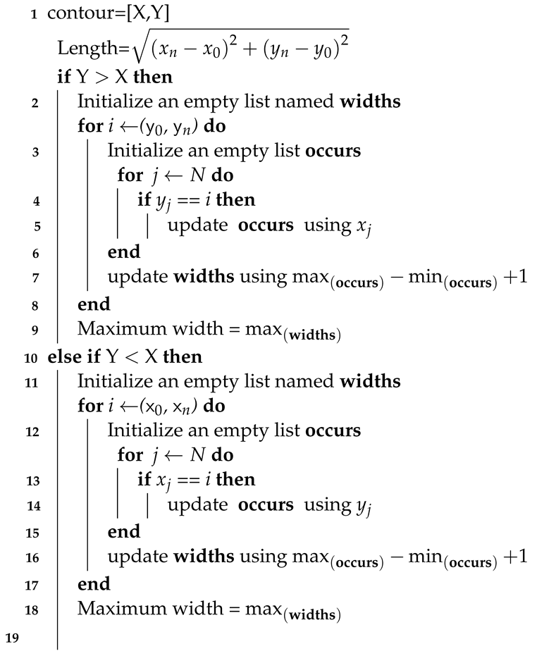
After extracting the individual crack objects from the previous step, this work calculated the cracks’ morphological features (length, width, area, and density). To calculate the length and the maximum width of the cracks, this work applied the Algorithm 1. From the previous section, this work has got the boundaries of the contours, i.e., cracks. Let a contour C=[X,Y] which is an array of two columns with N length, where, , ,......∈X denotes the rows of the image and , ,......∈Y denotes the columns of the image. Let (, ) and (, ) are the starting point and the ending point of the contour i.e. crack respectively. To find out the length of the crack, this work has calculated the distance between the starting point and the ending point of the crack boundary using the distance formula. After then for calculating the maximum width of a crack, this work first decided whether the crack is horizontal or longitudinal in nature based on the number of rows and columns of the image inside the contour. If the crack has more columns than rows, then the crack is horizontal type as its length is toward the horizontal direction of the image frame. On the other hand, a crack is longitudinal, if the contour has more rows. For finding the maximum with of a horizontal crack, this work has traversed from the starting column to the ending column of the crack boundary. During this crossing, this work has found out and stored the rows where any particular column has traveled in a list named occurs. This work estimated the number of rows traveled by any column when this searching loop was completed, and this work appended the results for each column to a list entitled widths. Finally, this work has searched for the maximum value in the list, and thus this work has calculated the maximum width of a crack. Furthermore, this work also estimated the location of the maximum with of the crack. For that, this work found the position of the first and last rows of the column which traveled maximum rows. For finding out the width of a longitudinal crack, this work utilized the same process, however, this time this work traversed through the rows from to and stored the number of columns traversed by a particular row . Later, based on these this work estimated the maximum number of columns traversed by a particular row , which represents the maximum width of a longitudinal crack. This work calculated the area of the contours as the area of the individual cracks. After that, this work added the area of the individual cracks and got the total area covered by the cracks in an image. Finally, this work divided the total area of the cracks by the number of pixels to get the density of the cracks in an image.
| Algorithm 1: Algorithm for length and width calculation |
 |
5. AMSEL Robot Working Method
The AMSEL robot platform conducts data collection and data processing fully autonomously. The working principle of the AMSEL platform is illustrated in Figure 9.
As it can be seen from Figure 9, the robotic system is divided into two working stations, i.e. robot device and the host computer. The AMSEL robot navigates on the concrete pavement and collects images from the surface. The robot collects images from a height of 30 cm and the covered area by one image is 302mm×227mm. After collecting the image data with a resolution of 640×480 pixels, the onboard computer of the AMSEL platform resizes the image in a resolution of 512×512 pixels and segments the cracks in the collected picture by utilizing the proposed deep-learning model described in Section 4.1. Then the robot transmits the processed image to the host computer in real-time. Finally, the host computer shows the image in the user interface of the robotic system and stores it on the device to further analyze the crack severity using the algorithm described in Section 4.3.
5.1. Manual Navigation and Pavement Inspection
In the manual mode, the robot’s movement and pavement inspection by a user from the user interface of the AMSEL robot system. The user interface has four navigation buttons, i.e. Forward, backward, Right, and left. The user navigates the robot using these buttons to the place where the user wants. For navigating manually, the user can control the speed of the robot as well by sending a specified velocity in RPM to the robot. The user has the flexibility to place the robot in any position and orientation in this manual mode. Figure 10 shows the manual inspection process in both indoor and outdoor environments. During the navigation, the user turns on the camera by pressing the "Video" button on the UI and checks whether there is a crack or not in a certain location by monitoring the Video display portion of the UI.
5.2. Automated Navigation and Pavement Inspection
In the automated navigation process, the AMSEL robot navigates through a predefined survey area. The navigation area is a rectangle with a width a meter and a length b meter, where the robot takes a,b as input from the user interface at the host computer. When the receives inputs and commands to move autonomously, it starts navigating automatically and collecting data lane by lane. The number of lanes depends on the width of the survey area. Figure 11 diagram of the survey area.
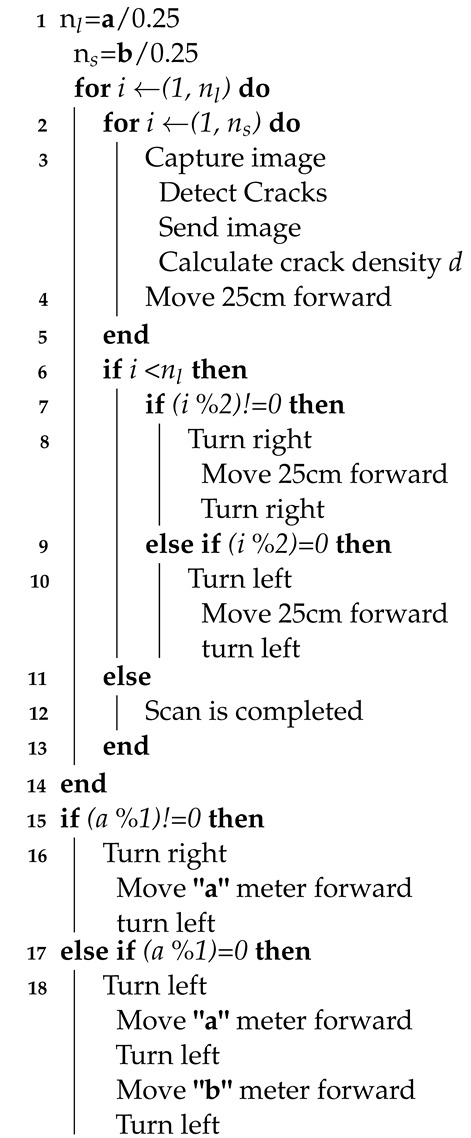
The AMSEL robot follows the stop-and-go a certain distance method for conducting the pavement inspection process. In this work, the AMSEL robot goes for each
25cm and stops to collect NDE data. The distance between two consecutive lanes is also selected as 25cm in this work. Algorithm 2 displays the method of the
AMSEL robot’s automated navigation and pavement procedure respectively. Figure 12 shows the
automated inspection process in the outdoor environment. From Algorithm 2 it can be seen that, after getting the command of the automated navigation, the AMSEL
robot calculates the number of lanes n1 and the number of steps ns in each lane. The number of lanes n1 is determined
by dividing the width a of the survey area by 0.25 as the distance between two lanes is 25cm. And the number of steps ns is determined by dividing the length of the survey area by 0.25 as the robot will move 25cm in each step. Then the robot starts performing the assigned tasks in the steps. First, the robot captures one picture and detects cracks in that. After detecting cracks in the picture, the picture is transferred to the host computer along with the robot location on the survey grid and the density of cracks in the image. Then the robot directly moves to the next scanning location. For navigating the correct distance and placing the robot in the precise position, this work has calibrated the spatial encoder data of the motors. After calibration, this work found that for moving 1 meter, wheels change their position by 1176 points.
Based on this, this work calculated the value for navigating 25cm. By considering the change in position of the wheels, this work has calibrated for left and right turn by 90∘ also. When the robot completes all the steps on a lane, it checks whether it is an odd or even lane. If it is an odd lane, the robot turns right, moves 25cm, and turns right again for placing itself at the beginning of the next lane. On the other hand, if the lane is an even lane, the robot turns left, moves 25cm, and turns left again to place it at the beginning of the next lane. The robot continues these processes till it completes scanning the last lane. After completing the last lane, it again checks whether the last is odd or even. If the last lane is odd, the robot turns left, and navigates the a meter distance, turns left again, and navigates the b meter distance. After this, it makes a 360∘ turn to go back to the starting position and orientation of the robot. On contrary, if the final lane is even, the robot turns right, navigates the ameter distance, and turns right again to go back to the starting position and orientation of the robot.
| Algorithm 2: Algorithm for automated navigation and inspection |
 |
6. Results & Discussion
6.1. Performance of the Deep Learning Model
This work has used one segmentation model named RCDNet for predicting the images. For evaluating the performance of our proposed RCDNet this work used four metrics: Accuracy, Intersection over Union, Dice loss, and Dice coefficient. The percentage of successfully categorized pixels is referred to as pixel accuracy while a binary segmentation task is being performed. However, due to the class imbalance issue, pixel accuracy is not the best metric to evaluate the segmentation task. For the majority of the Non-lane pixels in the case of lane detection, the images in the dataset are severely unbalanced. The Dice coefficient and the IOU, on the other hand, are seen to be more useful metrics because they depend on the overlap between the anticipated picture and the ground truth image. The metrics can be mathematically represented using the following equation.
The calculation demonstrates that the Dice coefficient represents the sum of the pixels in the two overlapping regions. The IOU also stands for the region of overlap between the expected and actual images, which is delineated by the union area. Figure 13 displays the accuracy, loss, Dice coefficient, and IoU trend for our proposed model over the epochs of both the training and test sets.
From Figure 13 it can be seen that our model has been trained well. There is not so much difference in the curves of the training set and test set which indicates that the model did not experience underfit or overfit. The training curves for all the metrics did not fluctuate throughout all the epochs. Between the first and about the third epochs of our model, the test curves began to rise quickly. But from the third epoch, it gradually increased and began to stabilize. But around the 27th, 52nd, 84th, and 97th, they went through four minor oscillations of varying degrees. However, our model was able to handle this variation and starting with the very next epochs, the curves stabilized once more. Finally, our model showed promising results in terms of metrics. Table 3 presents the result of our developed model from the perspective of the previously mentioned metrics on both the train set and the test set.
6.2. Pavement Assessment in Manual Mode
For the manual assessment of the pavement, the AMSEL robotic platform was navigated by an operator both in indoor and outdoor environments. The robot moved in different places and collected pictures using its visual sensor. The onboard computer segmented the crack pixels and sent the predicted images to the ground stations. After getting the segmented results from the RCDNet, this work measured the length, width, area, and density of the cracks. Though the crack measurement algorithm produces the result in a pixel unit, the size of the cracks in the physical unit can be calculated easily. As the vision sensor of the robotic system can cover an area of 302mm×227mm with a pixel resolution of 640×480; 1 pixel is about 0.47mm both in height and width of the picture. Furthermore, this work compared these results with manually measured data. In this study, the severity of the cracks was also been assessed. The density of the cracks was calculated as the ratio of the cracked pixels and the total pixels of an image. The severity scale density used in this work is shown in Table 4.
Figure 14 and Figure 15 show the original images, predicted black and white images, overlapped images, and the images after the crack measurement algorithm in indoor and outdoor environments respectively. Table 5 and Table 6 show the comparison between the manually collected data and the digitally extracted data from the as well as show the severity in indoor and outdoor environments respectively.
For indoor, from Figure 14, it can be seen that all the cracks are well predicted in the indoor environment. Even in the presence of shadow (Image2, Image3, Image5), and external noise (Image9) the RCDNet model detects the cracks accurately. However, if this work observes Image2, Image8, and Image10 very closely, it can be noticed that there is some discontinuity in the detection. A very little portion of the cracks is not detected in the images. This work manually measured the widths of those portions and found the limitation of our proposed RCDNet, it can not detect cracks with widths less than 1mm from 30cm height. From Table 5, it can be seen that the difference between the manually measured data (length, width) and digitally measured data of the cracks is very small for the indoor images. This work has found that the average error rate of the measurements is 2.219% and 6.155% respectively for the length and maximum width. One finding is that the table shows more errors in the case of width calculation. However, this work believes that this large error was due to the ambiguity of determining cracks with the scale by the naked eye.
For outdoor, from Figure 15, it can be seen that all the images are predicted accurately. However, if this work takes a closer look at Image12, Image13, Image14, and Image19 there is little misprediction. From Image12, the finding is that, when the sunshine is so extreme and there is a dark shadow, our model may mispredict the Shadowline as a crack. In Image13 and Image19 little portions of the cracks are not detected. The problem this work has here is that the depth between the edges of the cracks is very small, which does not look like a crack rather than a scratch on the pavement. However, the overall prediction in the outdoor environment is also quite accurate. From Table 6, it can be seen that the difference between the manually measured data and digitally measured data is also very small in the outdoor images like the indoor images. The relative error rate of the measurements is 6.703% and 5.631% respectively. The unexpected finding from this table is the error rate in the length calculation. However, this work can observe that Image19 which has two cracks, is not predicted accurately due to the less depth and shows a bigger deviation in error. And this deviation affects the average error rate badly.
This work has also performed a linear regression between manually measured and digitally measured length as well as the width of the cracks to check the stability of digitally measured data both for indoor and outdoor data. The linear regression for both indoor data and outdoor data in Figure 16 (a,b) and Figure 16 (c, d) show that the value of R2 in both cases (i.e. length, width) is close to 1. Besides this, the worthy finding is that the regression efficiency for both data is also close to 1. This clearly indicates that the proposed system has good absolute accuracy for crack length and width measurement.
In the case of the severity, from indoor images, this work found that among the ten images, four images are in severe condition. Among the severe cracks, Image 5 is the most severe (6% cracked). Of the other images, five images are in poor crack condition and one image is in fair crack condition. From the outdoor images, this work found that all the cracks are in severe condition. Among them, Image 4 is in the highest rank (5.12% severe).
6.3. Pavement Assessment in Automated Mode
The autonomous pavement assessment of the AMSEL robot was tested in both indoor and outdoor environments. For the automated assessment of the AMSEL robot in an indoor environment, this work has chosen a 3m×2m grid in the parking lot of Dong-A University, Busan, South Korea. For inspecting the 3m×2m grid, the AMSEL robot takes around 10 minutes. For the outdoor, this work has chosen a 2.5m×1m grid in the outdoor parking lot of Dong-A University, Busan, South Korea. For inspecting the 2.5m×1m grid, the AMSEL robot takes around 6 minutes, which is way faster than manual inspection. In the indoor and outdoor environment, the robot collected and predicted 108 and 50 images respectively. Figure 17 and Figure 18 show the stitched picture after segmenting the cracks of each location in indoor and outdoor environments respectively.
The AMSEL robot platform also calculates the area of the cracks in each image and the density of the cracks to show the severity of each location. The area and severity of each location indoor and outdoor are illustrated in Fig Figure 19 (a), (b) and Figure 19 (c), (d).
By analyzing Fig Figure 19 (a), (b) and (c), (d), this work has found the severity statistics and the most severe location both in the indoor and outdoor grid respectively. Table 7 and Table 8 show the statistics of the detected cracks in the indoor and outdoor grid respectively.
From Table 7, it can be seen that among the 108 images total of 43 images contain cracks on the indoor grid. Among the cracks, the crack in the location of the first lane, the first stoppage has a maximum area of 3841.995mm2, and the crack in the location of the last lane, the last stoppage has a minimum area of 38.305mm2. The total cracked area is 22617.69mm2 and the grid is 0.38% cracked of its total area. From Table 8, it can be seen that among the 50 images total of 18 images contain cracks on the grid. Among the cracks, the crack in the location of the third lane, the first stoppage has a maximum area of 1741.35mm2, and the crack in the location of the fourth lane, the second stoppage has a minimum area of 308.20252. The total cracked area is 15231.88mm2 and the grid is 0.60% cracked of its total area.
7. Conclusions
In this work, a semi-automated robotic platform named AMSEL has been reported for inspecting pavement cracks in real-time. An encoder-decoder-based lightweight deep learning model named RCDNet was proposed to detect pavement cracks. The robotic platform was developed for manual and automated navigation to complete the inspection. Both indoors and outdoors, the robot was able to navigate and collect as well as analyze the data accurately. Extensive testing and deployment of the AMSEL showed the advantage over manual testing during pavement crack inspection and evaluation. The crack severity map was also generated based on the analysis of image data from the robot for providing a simple and efficient way to monitor pavement cracks. In future work, this work plans to integrate NDE sensors including IE, GPR, USW, ER, etc. Besides these, this work wants to add multiple visual sensors for covering a large area quickly to make the inspection process faster. Finally, our plan is to fuse all sensor data and develop a deep-learning model to obtain various defect information and construct a correlation model among the NDE sensors.
Author Contributions
Conceptualization, Md. Al-Masrur Khan, and Seong-Hoon Kee; Formal analysis, Md. Al-Masrur Khan, Regidestyoko Wasistha Harseno, Abdullah-Al Nahid, and Seong-Hoon Kee; Funding acquisition, Seong-Hoon Kee; Investigation, Md. Al-Masrur Khan, Abdullah-Al Nahid and Seong-Hoon Kee; Methodology, Md. Al-Masrur Khan, and Regidestyoko Wasistha Harseno; Software, Md. Al-Masrur Khan, and Regidestyoko Wasistha Harseno; Supervision, Seong-Hoon Kee; test, Md. Al-Masrur Khan, and Regidestyoko Wasistha Harseno; Visualization, Md. Al-Masrur Khan, Regidestyoko Wasistha Harseno, Abdullah-Al Nahid, and Seong-Hoon Kee; Writing—original draft, Md. Al-Masrur Khan; Writing—review & editing, Md. Al-Masrur Khan, Regidestyoko Wasistha Harseno, Abdullah-Al Nahid and Seong-Hoon Kee.
Funding
This work was supported by the Korea Institute of Marine Science and Technology Promotion (KIMST) grant funded by the Ministry of Oceans and Fisheries for the project titled ‘Development of smart maintenance monitoring techniques to prepare for disaster and deterioration of port infra structures’.
Institutional Review Board Statement
Not applicable.
Informed Consent Statement
Not applicable
Data Availability Statement
Not applicable.
Acknowledgments
The works in the paper were performed at the department of ICT integrated Ocean Smart Cities Engineering at Dong-A University, Busan, South Korea, when Md. Al-Masrur Khan was a master’s degree student at Dong-A University.
Conflicts of Interest
Not applicable.
References
- R. B. Lee, “Development of korean highway capacity manual,” Highway Capacity and Level of Service, pp. 233–238, 2021.
- C. Chen, H. Seo, C. H. Jun, and Y. Zhao, “A potential crack region method to detect crack using image processing of multiple thresholding,” Signal, Image and Video Processing, vol. 16, no. 6, pp. 1673–1681, 2022. [CrossRef]
- A. Akagic, E. Buza, S. Omanovic, and A. Karabegovic, “Pavement crack detection using otsu thresholding for image segmentation,” 2018 41st International Convention on Information and Communication Technology, Electronics and Microelectronics (MIPRO), 2018. [CrossRef]
- R. Nigam and S. K. Singh, “Crack detection in a beam using wavelet transform and photographic measurements,” Structures, vol. 25, pp. 436–447, 2020. [CrossRef]
- H. Zoubir, M. Rguig, M. El Aroussi, A. Chehri, and R. Saadane, “Concrete Bridge Crack Image classification using histograms of oriented gradients, uniform local binary patterns, and kernel principal component analysis,” Electronics, vol. 11, no. 20, p. 3357, 2022. [CrossRef]
- N. Gehri, J. Mata-Falcón, and W. Kaufmann, “Automated Crack Detection and measurement based on digital image correlation,” Construction and Building Materials, vol. 256, p. 119383, 2020. [CrossRef]
- R. Medina, J. Llamas, J. Gómez-García-Bermejo, E. Zalama, and M. Segarra, “Crack detection in concrete tunnels using a Gabor filter invariant to rotation,” Sensors, vol. 17, no. 7, p. 1670, 2017. [CrossRef]
- H.-N. Nguyen, T.-Y. Kam, and P.-Y. Cheng, “An automatic approach for accurate edge detection of concrete crack utilizing 2D geometric features of crack,” Journal of Signal Processing Systems, vol. 77, no. 3, pp. 221–240, 2013. [CrossRef]
- P. Chun, S. Izumi, and T. Yamane, “Automatic detection method of cracks from concrete surface imagery using two-step light gradient boosting machine,” Computer-Aided Civil and Infrastructure Engineering, vol. 36, no. 1, pp. 61–72, 2020. [CrossRef]
- A. Vedrtnam, S. Kumar, G. Barluenga, and S. Chaturvedi, “Early crack detection using modified Spectral Clustering Method assisted with FE analysis for distress anticipation in cement-based composites,” 2021. [CrossRef]
- L. Zhang, F. Yang, Y. Daniel Zhang, and Y. J. Zhu, “Road crack detection using deep convolutional neural network,” 2016 IEEE International Conference on Image Processing (ICIP), 2016. [CrossRef]
- Y.-J. Cha, W. Choi, and O. Büyüköztürk, “Deep learning-based crack damage detection using convolutional neural networks,” Computer-Aided Civil and Infrastructure Engineering, vol. 32, no. 5, pp. 361–378, 2017. [CrossRef]
- M. Eisenbach, R. Stricker, D. Seichter, K. Amende, K. Debes, M. Sesselmann, D. Ebersbach, U. Stoeckert, and H.-M. Gross, “How to get pavement distress detection ready for deep learning? A systematic approach,” 2017 International Joint Conference on Neural Networks (IJCNN), 2017. [CrossRef]
- Y. Li, Z. Han, H. Xu, L. Liu, X. Li, and K. Zhang, “Yolov3-Lite: A lightweight crack detection network for aircraft structure based on depthwise separable convolutions,” Applied Sciences, vol. 9, no. 18, p. 3781, 2019. [CrossRef]
- L. Li, S. Zheng, C. Wang, S. Zhao, X. Chai, L. Peng, Q. Tong, and J. Wang, “Crack Detection Method of sleeper based on Cascade Convolutional Neural Network,” Journal of Advanced Transportation, vol. 2022, pp. 1–14, 2022. [CrossRef]
- X. Yang, H. Li, Y. Yu, X. Luo, T. Huang, and X. Yang, “Automatic pixel-level crack detection and measurement using fully convolutional network,” Computer-Aided Civil and Infrastructure Engineering, vol. 33, no. 12, pp. 1090–1109, 2018. [CrossRef]
- V. Polovnikov, D. Alekseev, I. Vinogradov, and G. V. Lashkia, “DAUNet: Deep Augmented Neural Network for pavement crack segmentation,” IEEE Access, vol. 9, pp. 125714–125723, 2021. [CrossRef]
- P. Yong and N. Wang, “RIIAnet: A real-time segmentation network integrated with multi-type features of different depths for pavement cracks,” Applied Sciences, vol. 12, no. 14, p. 7066, 2022. [CrossRef]
- S.-N. Yu, J.-H. Jang, and C.-S. Han, “Auto inspection system using a mobile robot for detecting concrete cracks in a tunnel,” Automation in Construction, vol. 16, no. 3, pp. 255–261, 2007. [CrossRef]
- P. Oyekola, A. Mohamed*, and J. Pumwa, “Robotic model for unmanned crack and corrosion inspection,” International Journal of Innovative Technology and Exploring Engineering, vol. 9, no. 1, pp. 862–867, 2019. [CrossRef]
- H. Li, D. Song, Y. Liu, and B. Li, “Automatic pavement crack detection by multi-scale image fusion,” IEEE Transactions on Intelligent Transportation Systems, vol. 20, no. 6, pp. 2025–2036, 2019. [CrossRef]
- H. M. La, T. H. Dinh, N. H. Pham, Q. P. Ha, and A. Q. Pham, “Automated robotic monitoring and inspection of steel structures and Bridges,” Robotica, vol. 37, no. 5, pp. 947–967, 2018. [CrossRef]
- H. M. La, N. Gucunski, K. Dana, and S.-H. Kee, “Development of an autonomous bridge deck inspection robotic system,” Journal of Field Robotics, vol. 34, no. 8, pp. 1489–1504, 2017. [CrossRef]
- H. Kolvenbach, G. Valsecchi, R. Grandia, A. Ruiz, F. Jenelten, and M. Hutter, “Tactile inspection of concrete deterioration in sewers with legged robots,” in Proc. 12th Conf. Field Service Robot., 2019. [CrossRef]
- D. V. K. Le, Z. Chen, and R. Rajkumar, “Multi-sensors in-line inspection robot for pipe flaws detection,” IET Science, Measurement & Technology, vol. 14, no. 1, pp. 71–82, 2020. [CrossRef]
- B. Lei, Y. Ren, N. Wang, L. Huo, and G. Song, “Design of a new low-cost unmanned aerial vehicle and vision-based concrete crack inspection method,” Structural Health Monitoring, vol. 19, no. 6, pp. 1871–1883, 2020. [CrossRef]
- Y. Pan, X. Zhang, G. Cervone, and L. Yang, “Detection of asphalt pavement potholes and cracks based on the unmanned aerial vehicle multispectral imagery,” IEEE Journal of Selected Topics in Applied Earth Observations and Remote Sensing, vol. 11, no. 10, pp. 3701–3712, 2018. [CrossRef]
- R. Montero, E. Menendez, J. G. Victores, and C. Balaguer, “Intelligent robotic system for autonomous crack detection and caracterization in concrete tunnels,” 2017 IEEE International Conference on Autonomous Robot Systems and Competitions (ICARSC), 2017. [CrossRef]
- L. Yang, B. Li, W. Li, H. Brand, B. Jiang, and J. Xiao, “Concrete defects inspection and 3D mapping using CityFlyer Quadrotor Robot,” IEEE/CAA Journal of Automatica Sinica, vol. 7, no. 4, pp. 991–1002, 2020. [CrossRef]
- Z. Gui and H. Li, “Automated defect detection and visualization for the robotic airport runway inspection,” IEEE Access, vol. 8, pp. 76100–76107, 2020. [CrossRef]
- B. Ramalingam, A. A. Hayat, M. R. Elara, B. Félix Gómez, L. Yi, T. Pathmakumar, M. M. Rayguru, and S. Subramanian, “Deep learning based pavement inspection using self-reconfigurable robot,” Sensors, vol. 21, no. 8, p. 2595, 2021. [CrossRef]
- Z. He, S. Jiang, J. Zhang, and G. Wu, “Automatic damage detection using anchor-free method and unmanned surface vessel,” Automation in Construction, vol. 133, p. 104017, 2022. [CrossRef]
- L. Yang, B. Li, J. Feng, G. Yang, Y. Chang, B. Jiang, and J. Xiao, “Automated Wall-climbing robot for Concrete Construction Inspection,” Journal of Field Robotics, 2022. [CrossRef]
- , B. Xiong, X. Li, X. Sang, and Q. Kong, “A novel intelligent inspection robot with deep stereo vision for three-dimensional concrete damage detection and quantification,” Structural Health Monitoring, vol. 21, no. 3, pp. 788–802, 2021. [CrossRef]
- F. Yang, L. Zhang, S. Yu, D. Prokhorov, X. Mei, and H. Ling, “Feature pyramid and hierarchical boosting network for pavement crack detection,” IEEE Transactions on Intelligent Transportation Systems, vol. 21, no. 4, pp. 1525–1535, 2020. [CrossRef]
Figure 1.
AMSEL robot configuration on the lab environment.
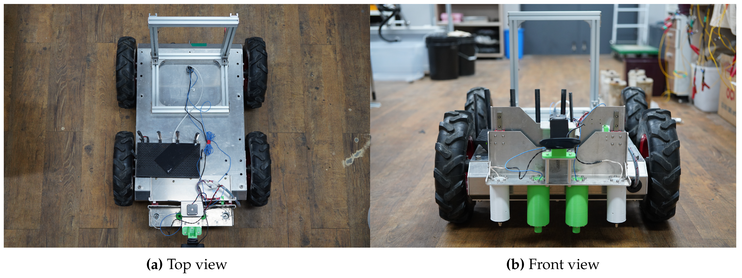
Figure 2.
Mechanical components of AMSEL.
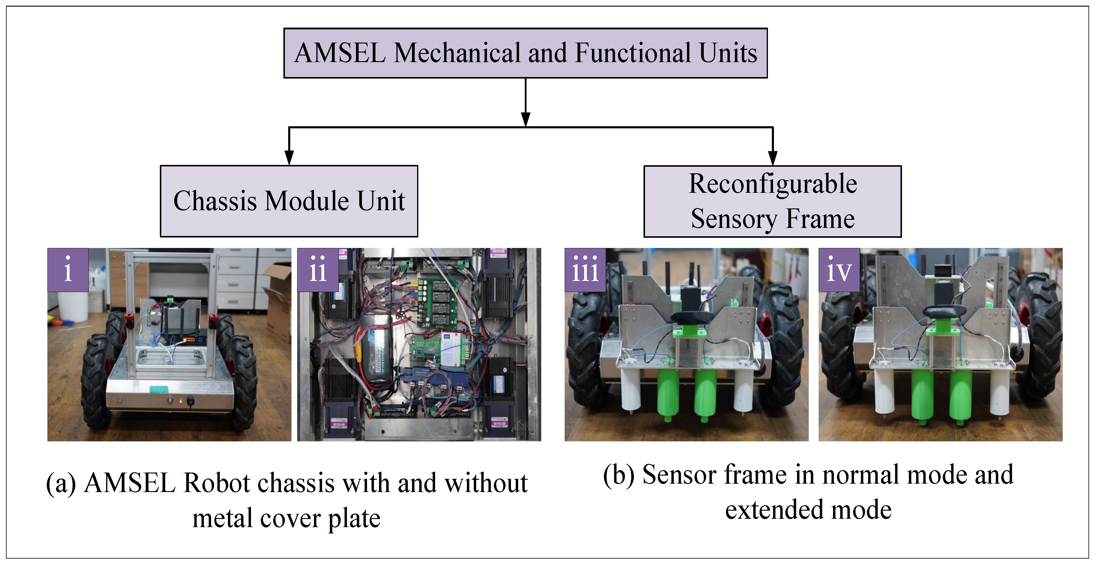
Figure 3.
Sensory, electrical, programming, and control units in AMSEL.
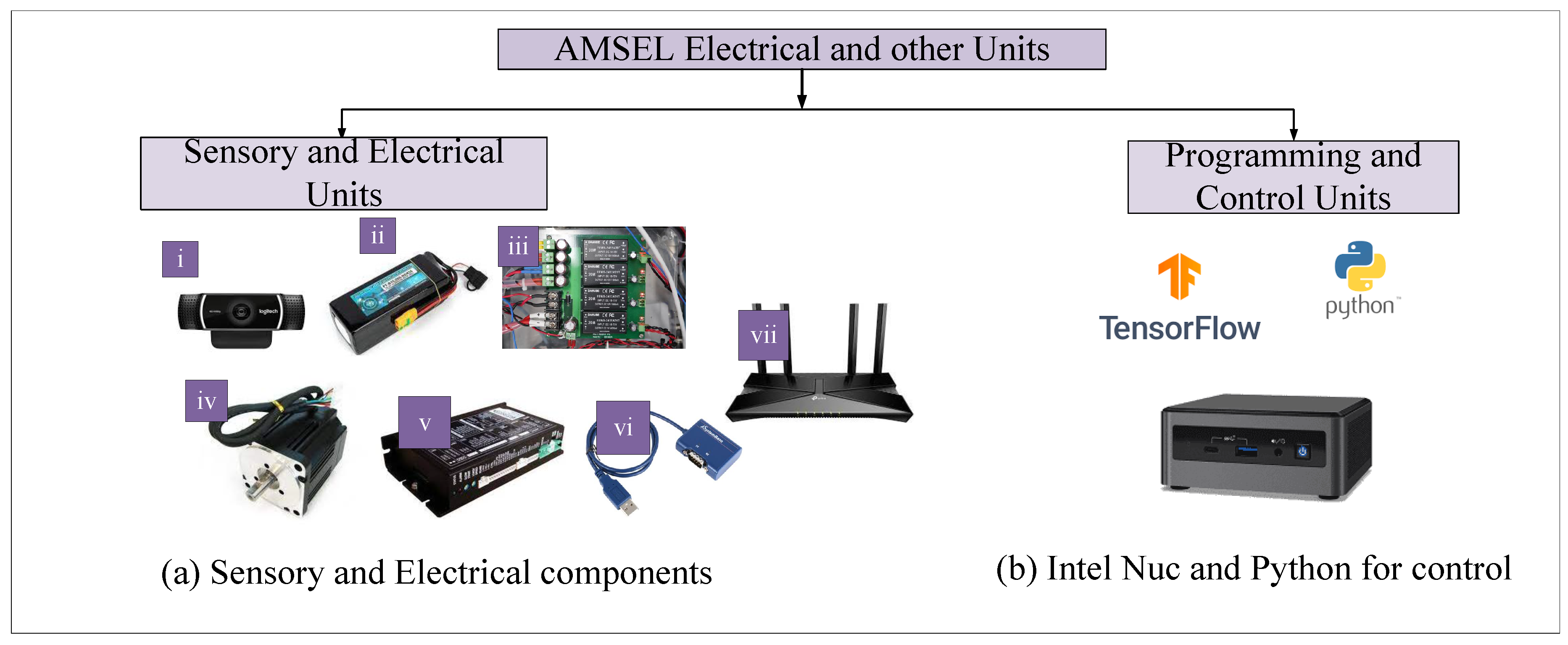
Figure 4.
Illustration of the graphical user interface for controlling the AMSEL robot.
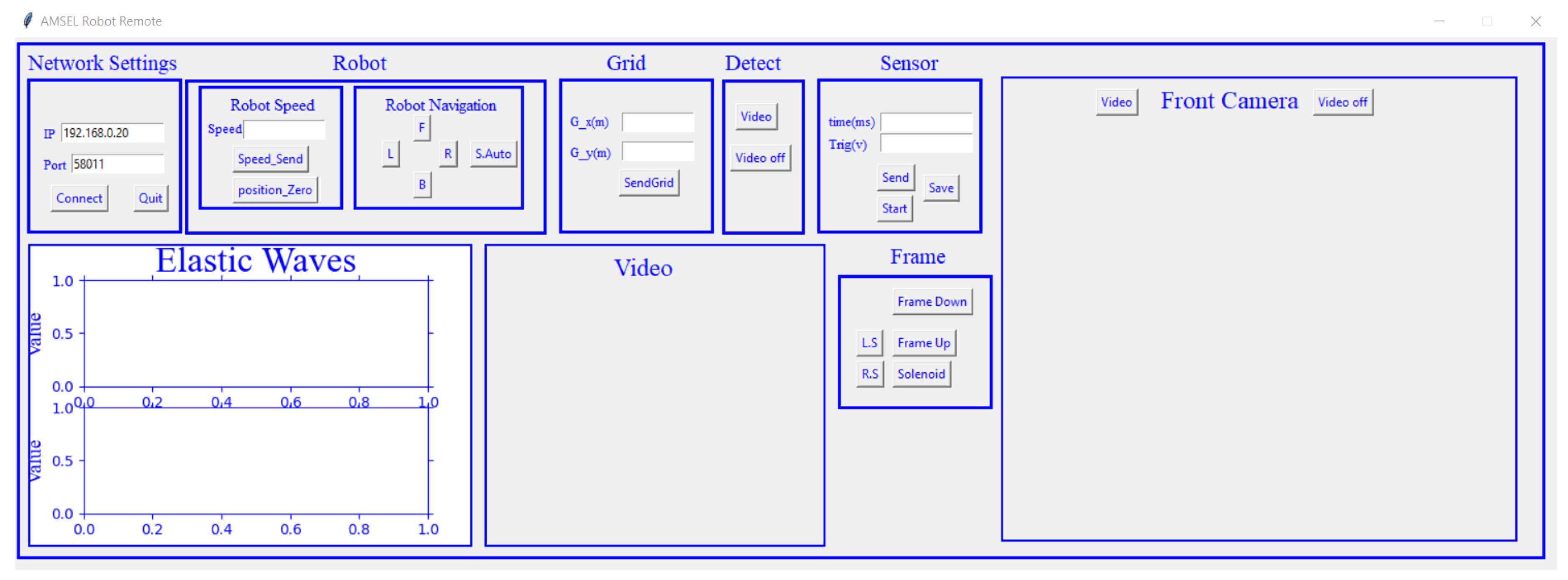
Figure 5.
Hardware architecture of AMSEL robot.
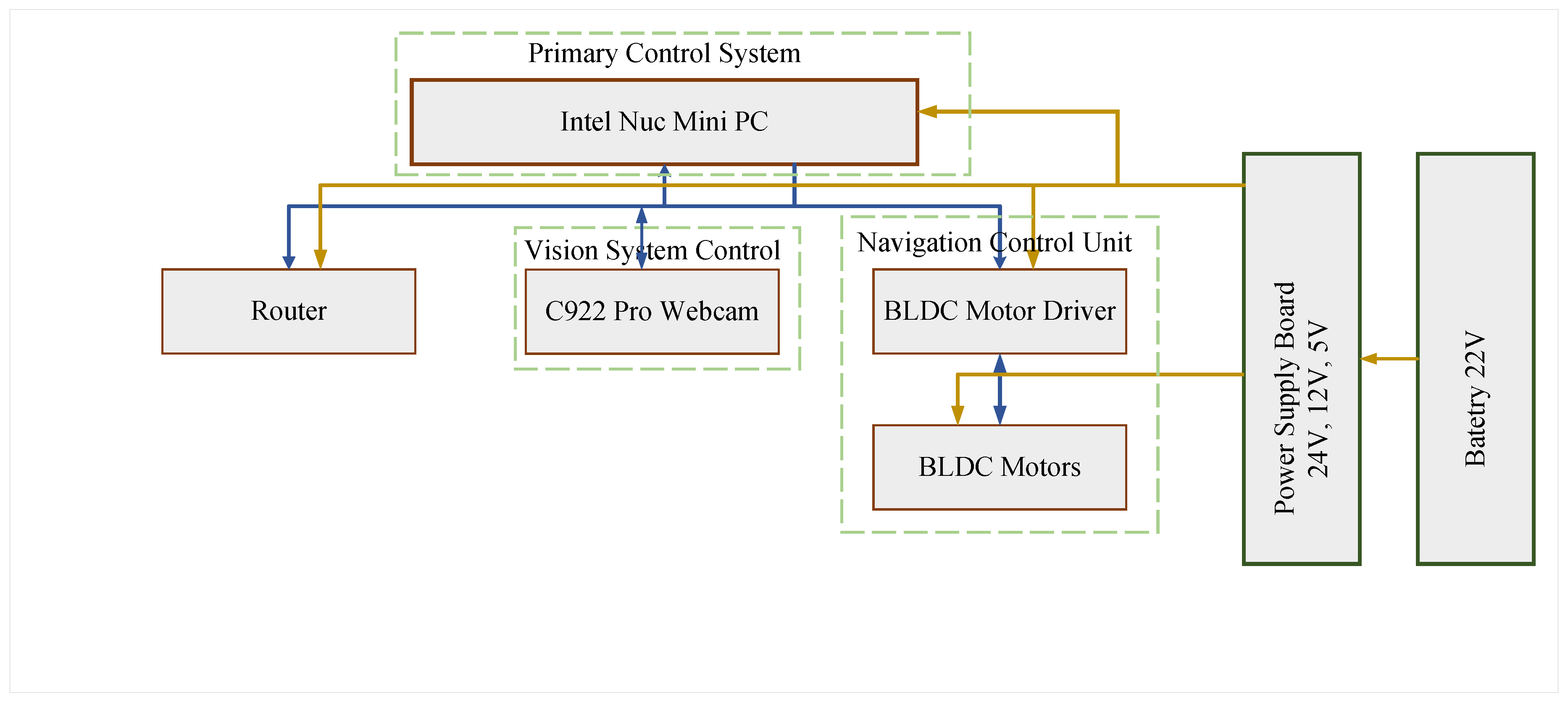
Figure 6.
Structure of the Proposed model.
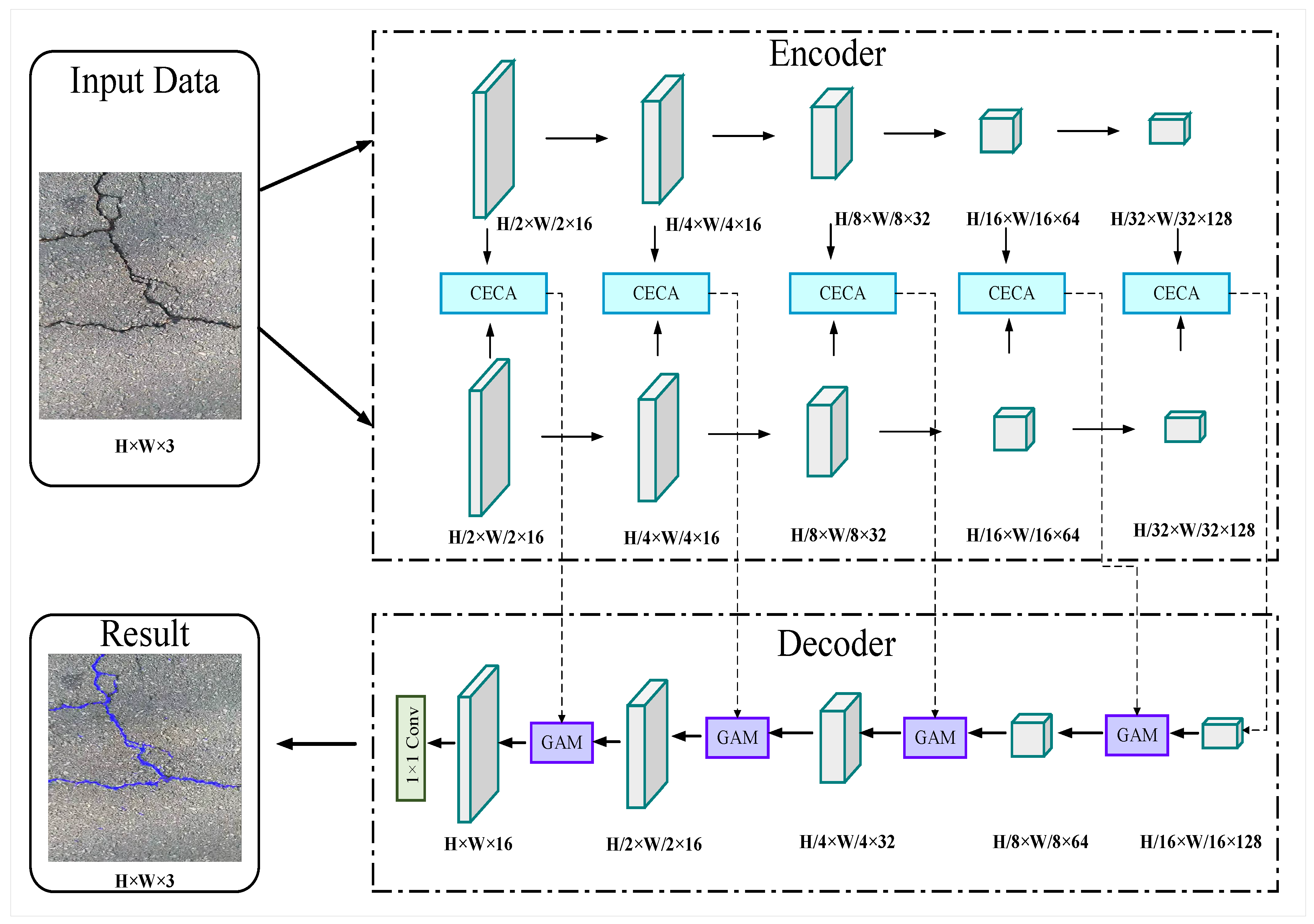
Figure 7.
CECA module structure.
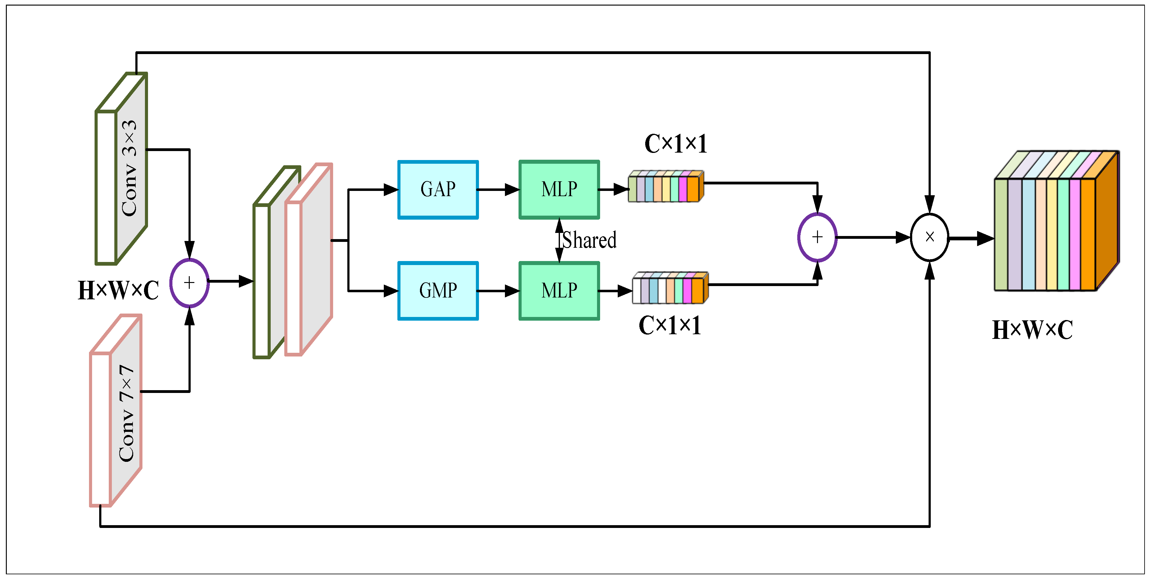
Figure 8.
GAM module structure.
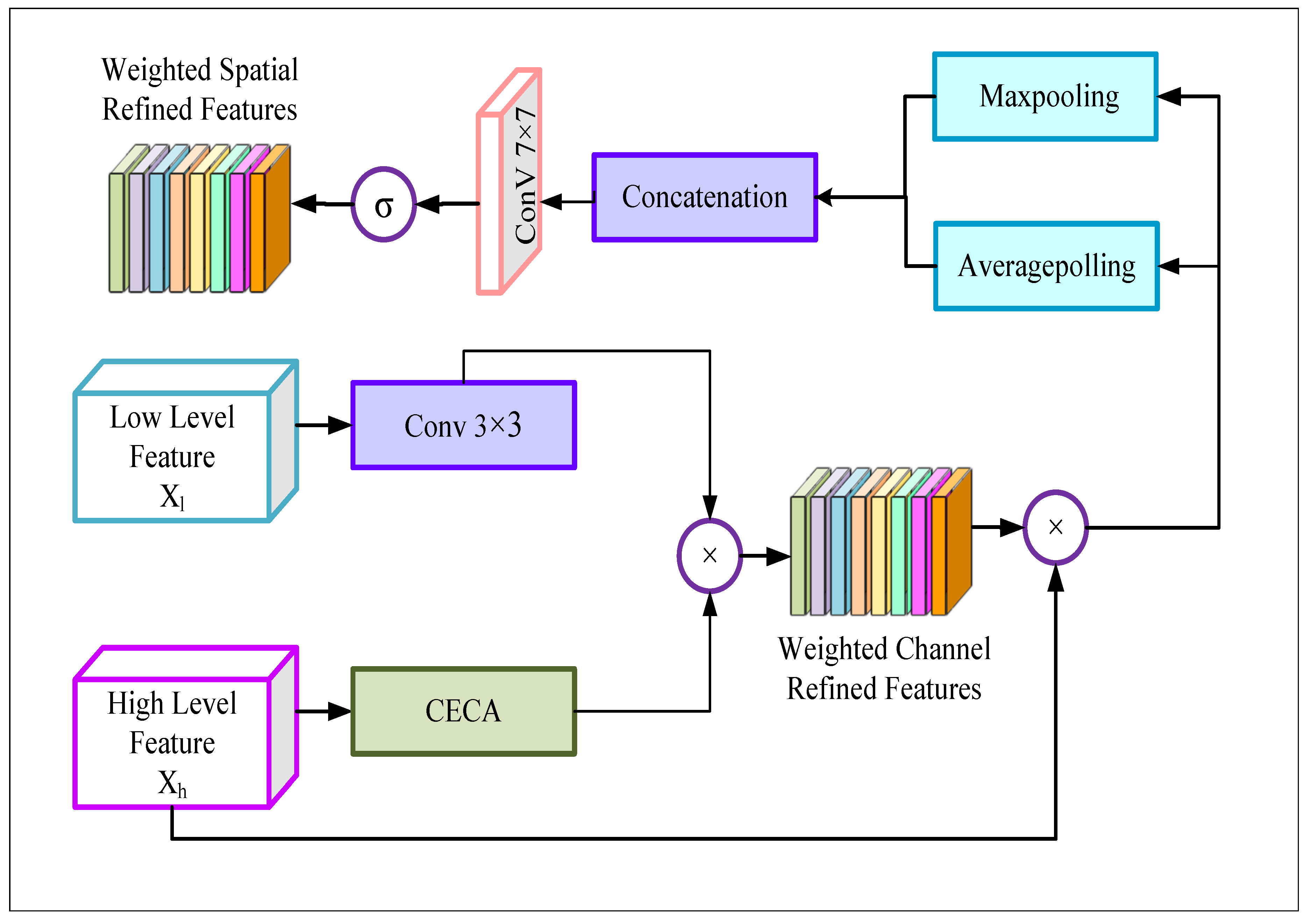
Figure 9.
The working principle of the AMSEL robot navigation inspection system.
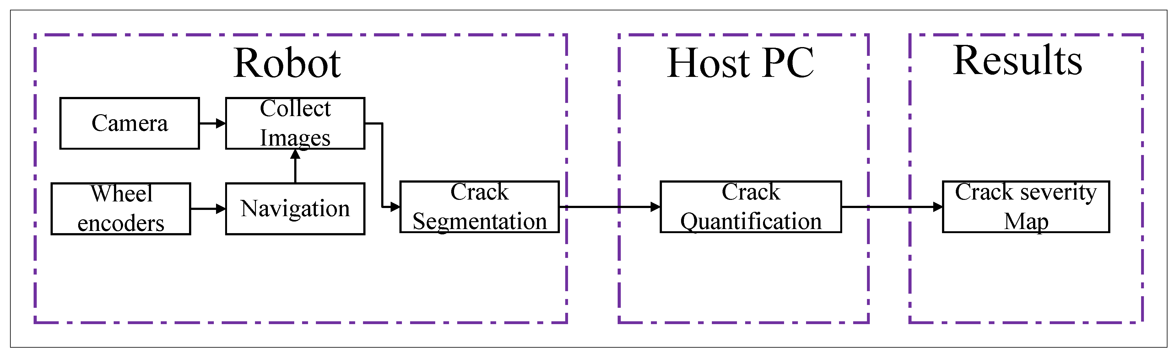
Figure 10.
Manual navigation and data collection in the indoor and outdoor environment.
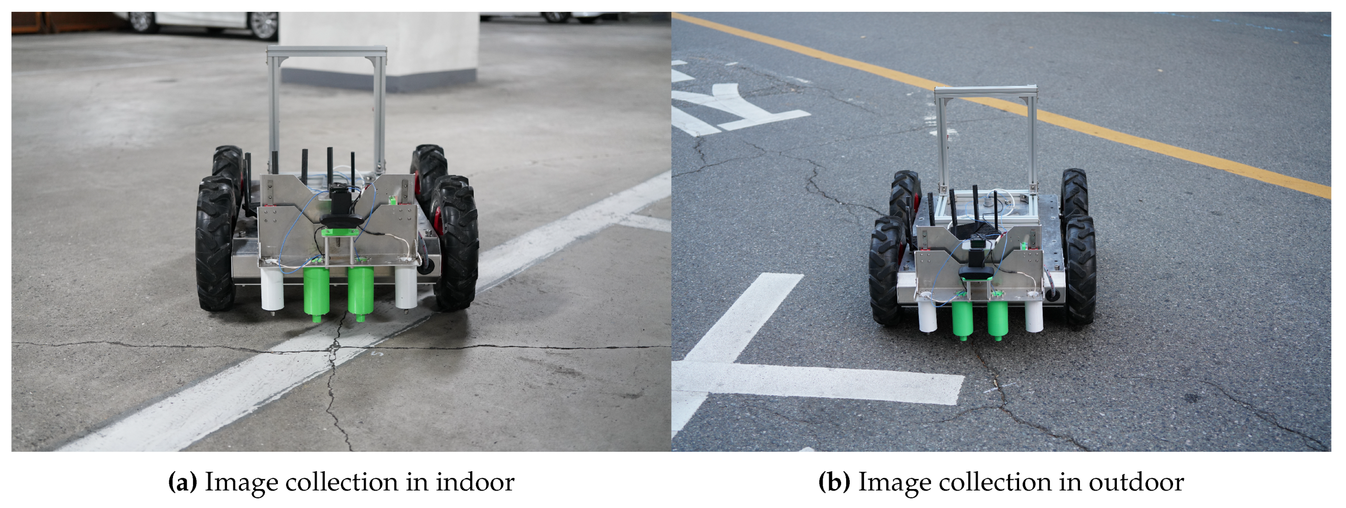
Figure 11.
The diagram of survey area for the AMSEL robot.
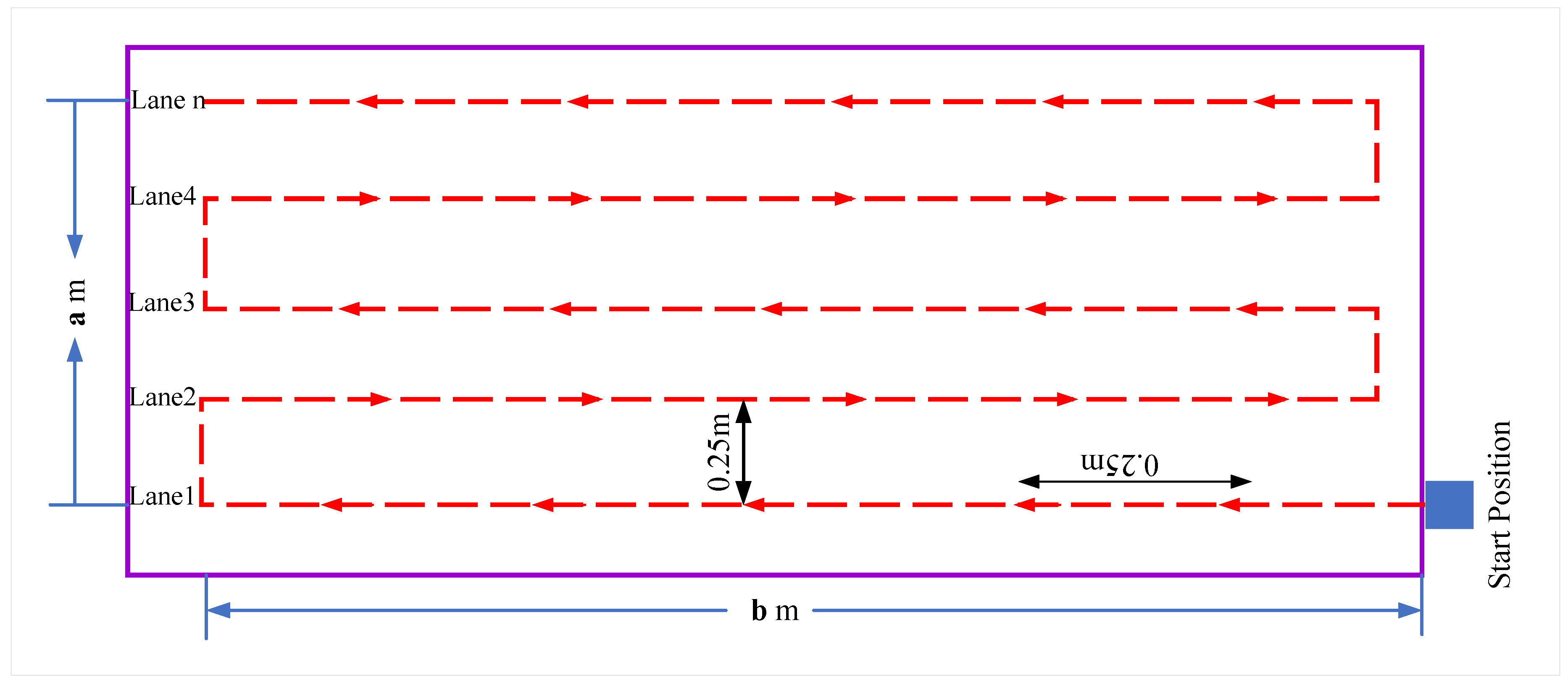
Figure 12.
Automated navigation and data collection in the indoor and outdoor environment.
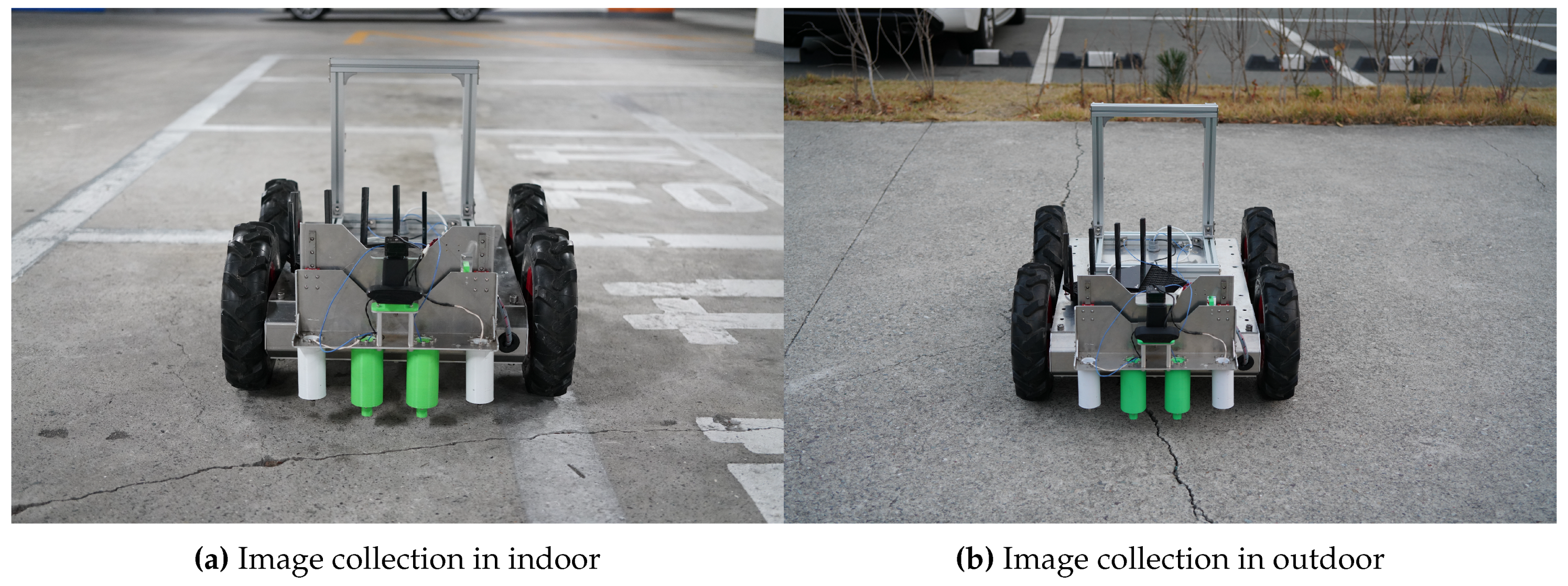
Figure 13.
Curves of accuracy, loss, dice coefficient, and IoU while training and testing the models at 100 epochs.
Figure 13.
Curves of accuracy, loss, dice coefficient, and IoU while training and testing the models at 100 epochs.
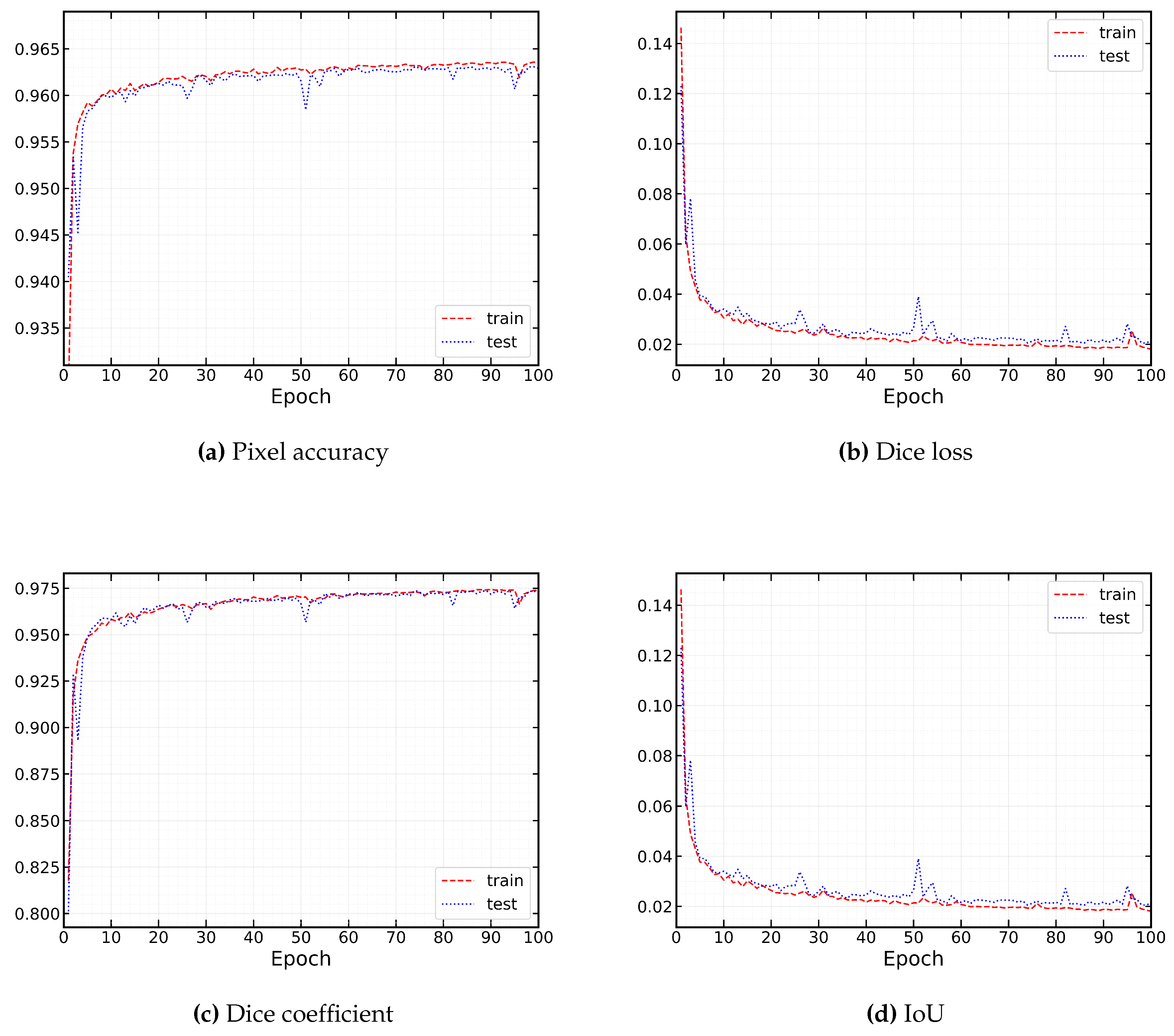
Figure 14.
Manually collected images from indoors. (a) Original Image (b) Predicted black and white images (c) Overlapped images (d) Images showing the location of maximum width
Figure 14.
Manually collected images from indoors. (a) Original Image (b) Predicted black and white images (c) Overlapped images (d) Images showing the location of maximum width
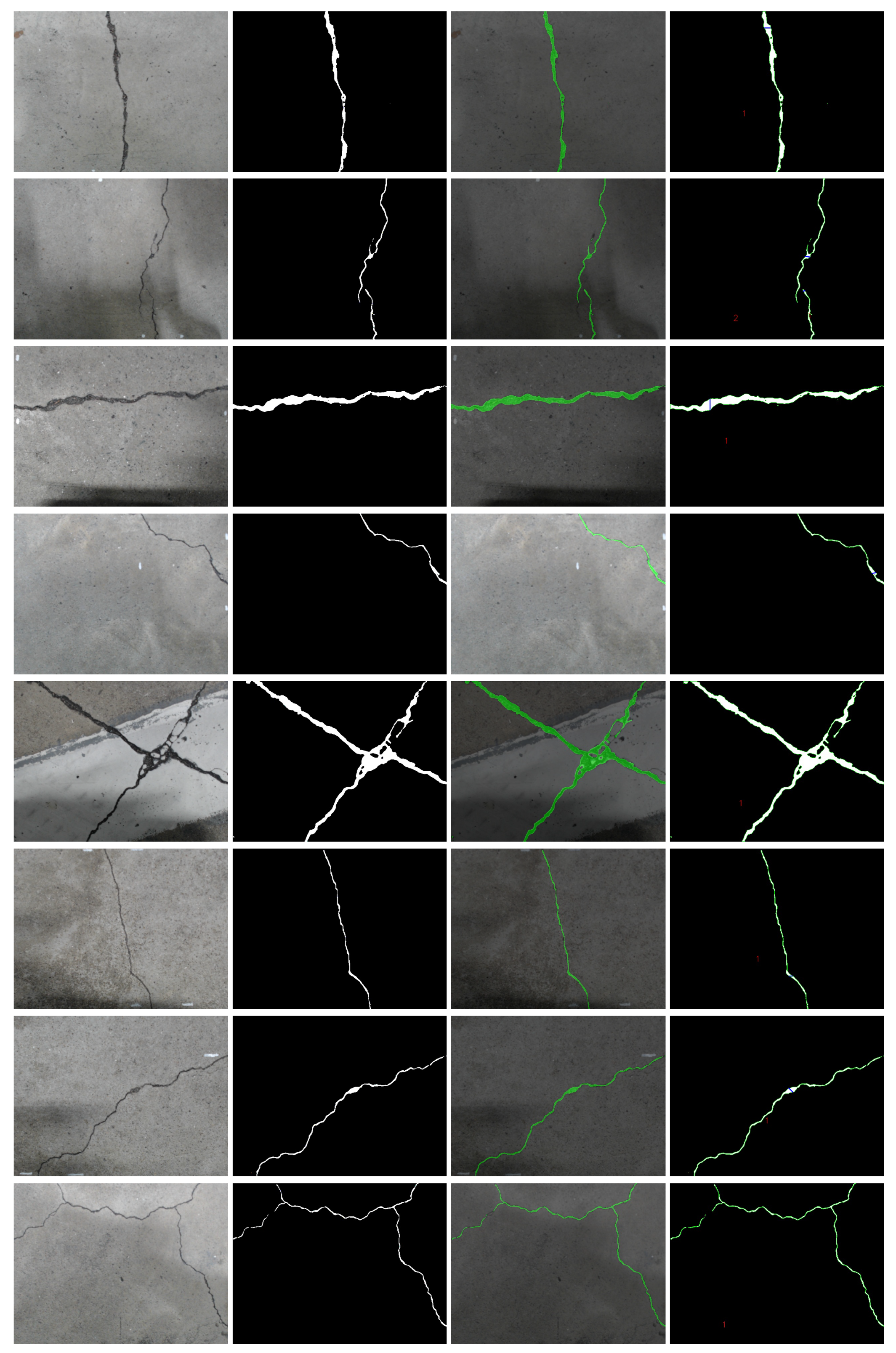
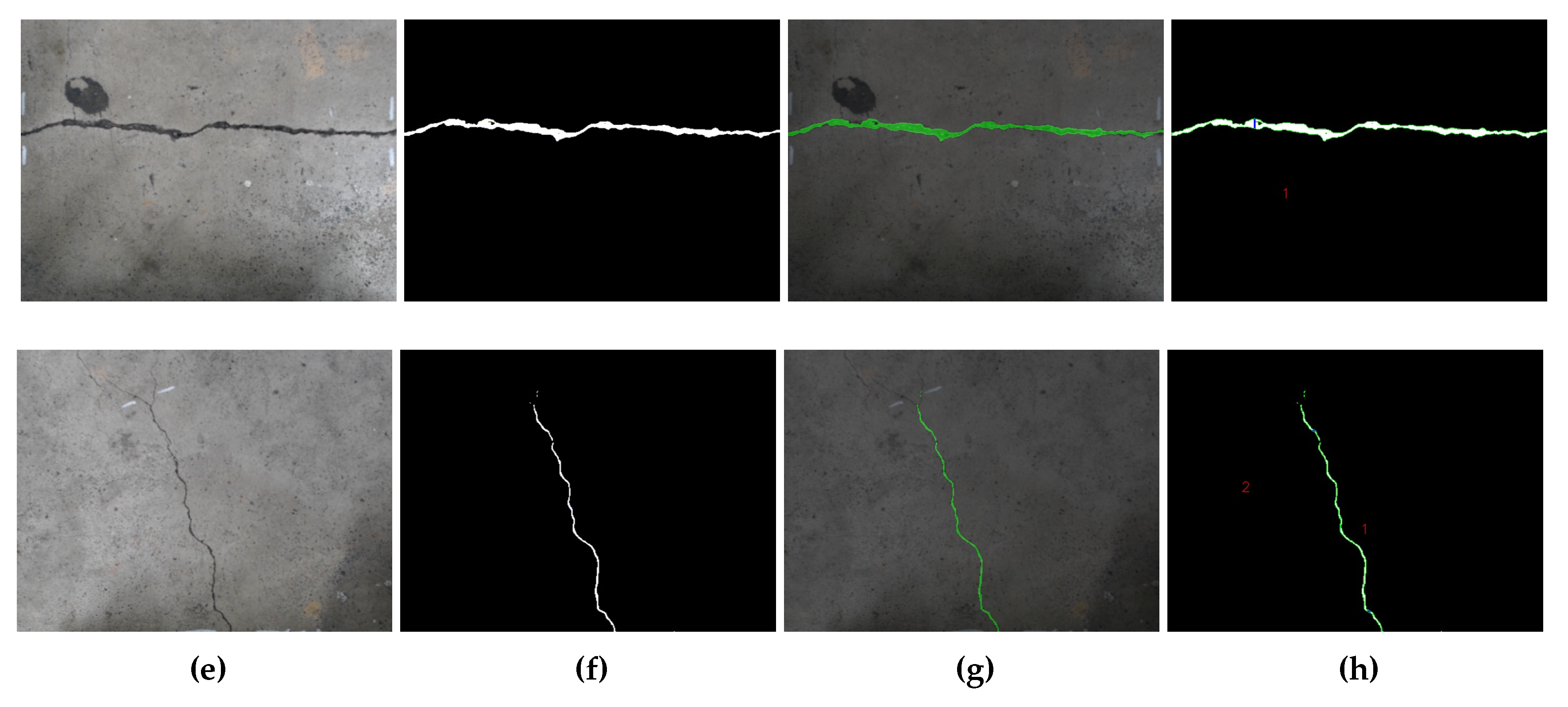
Figure 15.
Manually collected images from outdoors. (a) Original Image (b) Predicted black and white images (c) Overlapped images (d) Images showing the location of maximum width
Figure 15.
Manually collected images from outdoors. (a) Original Image (b) Predicted black and white images (c) Overlapped images (d) Images showing the location of maximum width
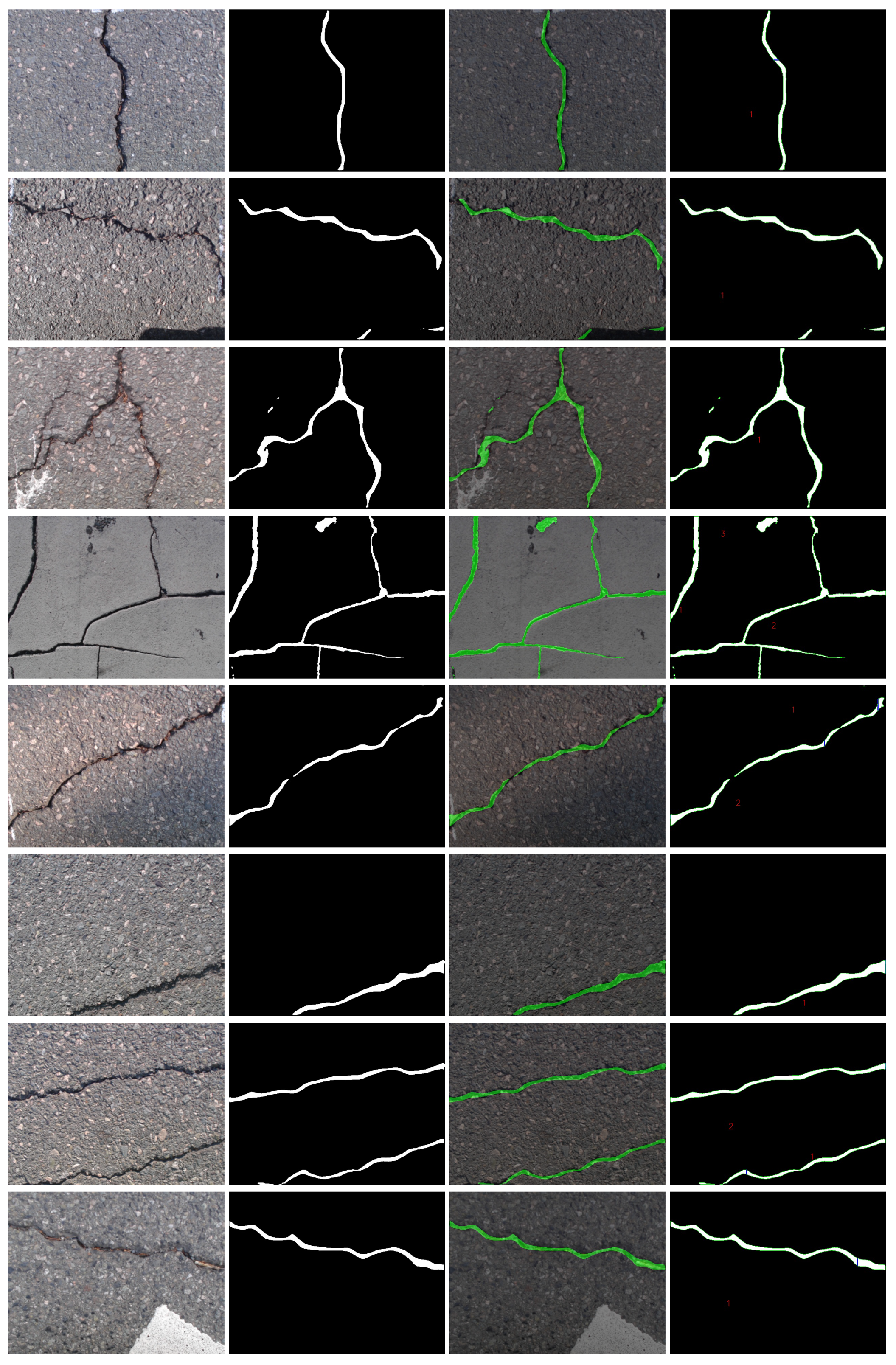
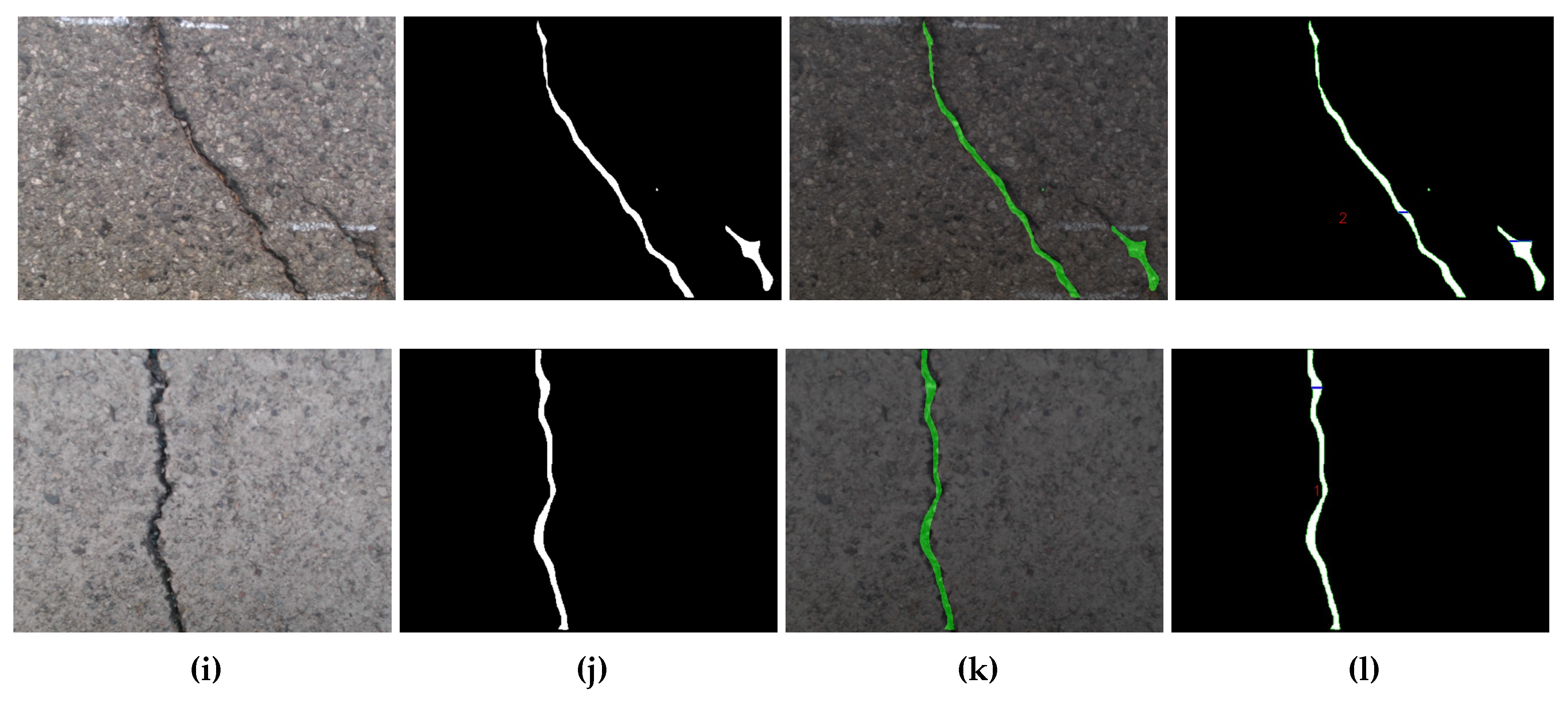
Figure 16.
Manual measurement vs digital measurement: (a) length in indoor, (b) width in indoor, (c) length in outdoor, (d) width in outdoor
Figure 16.
Manual measurement vs digital measurement: (a) length in indoor, (b) width in indoor, (c) length in outdoor, (d) width in outdoor
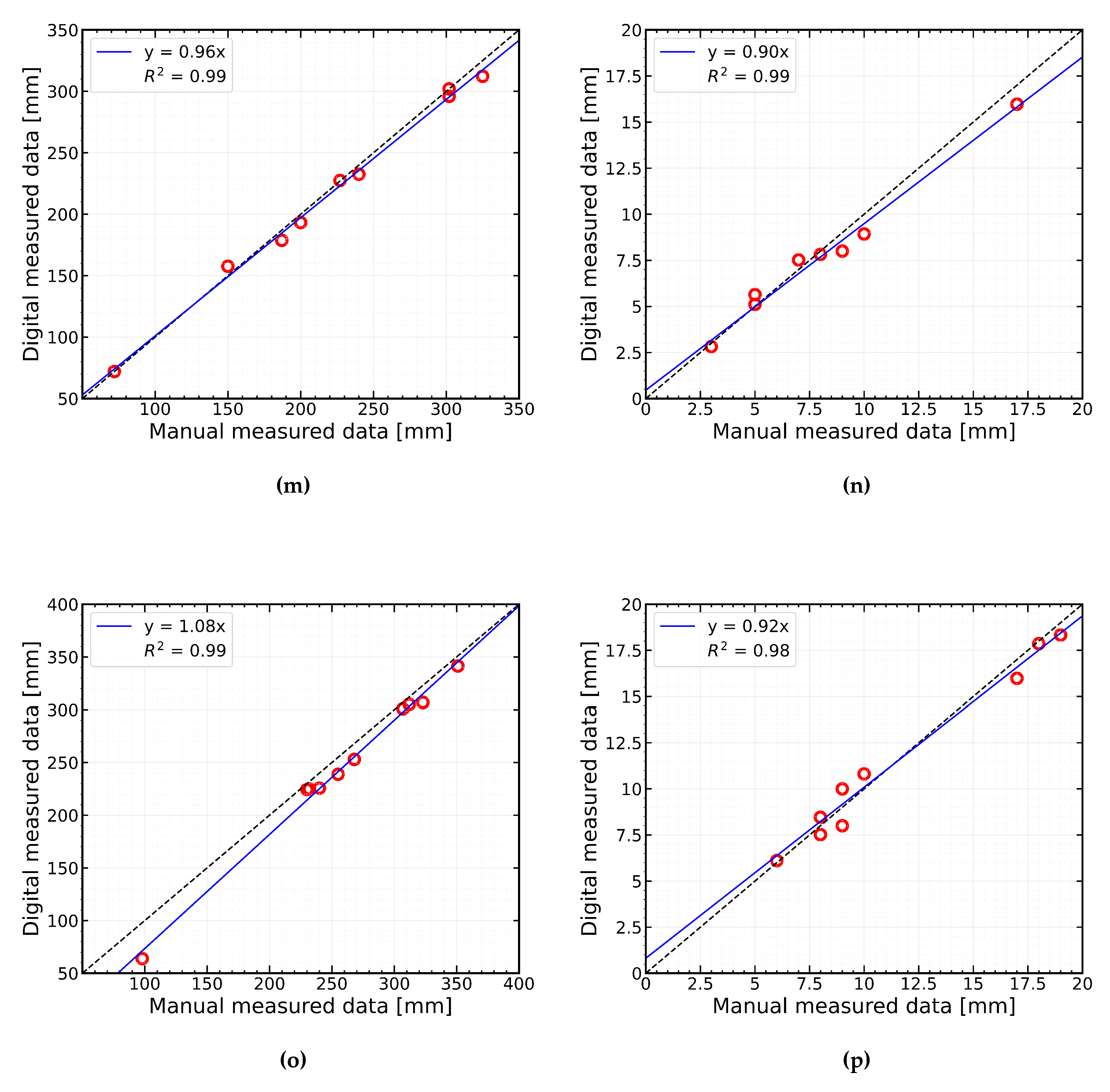
Figure 17.
Stitched image collected from the indoor.
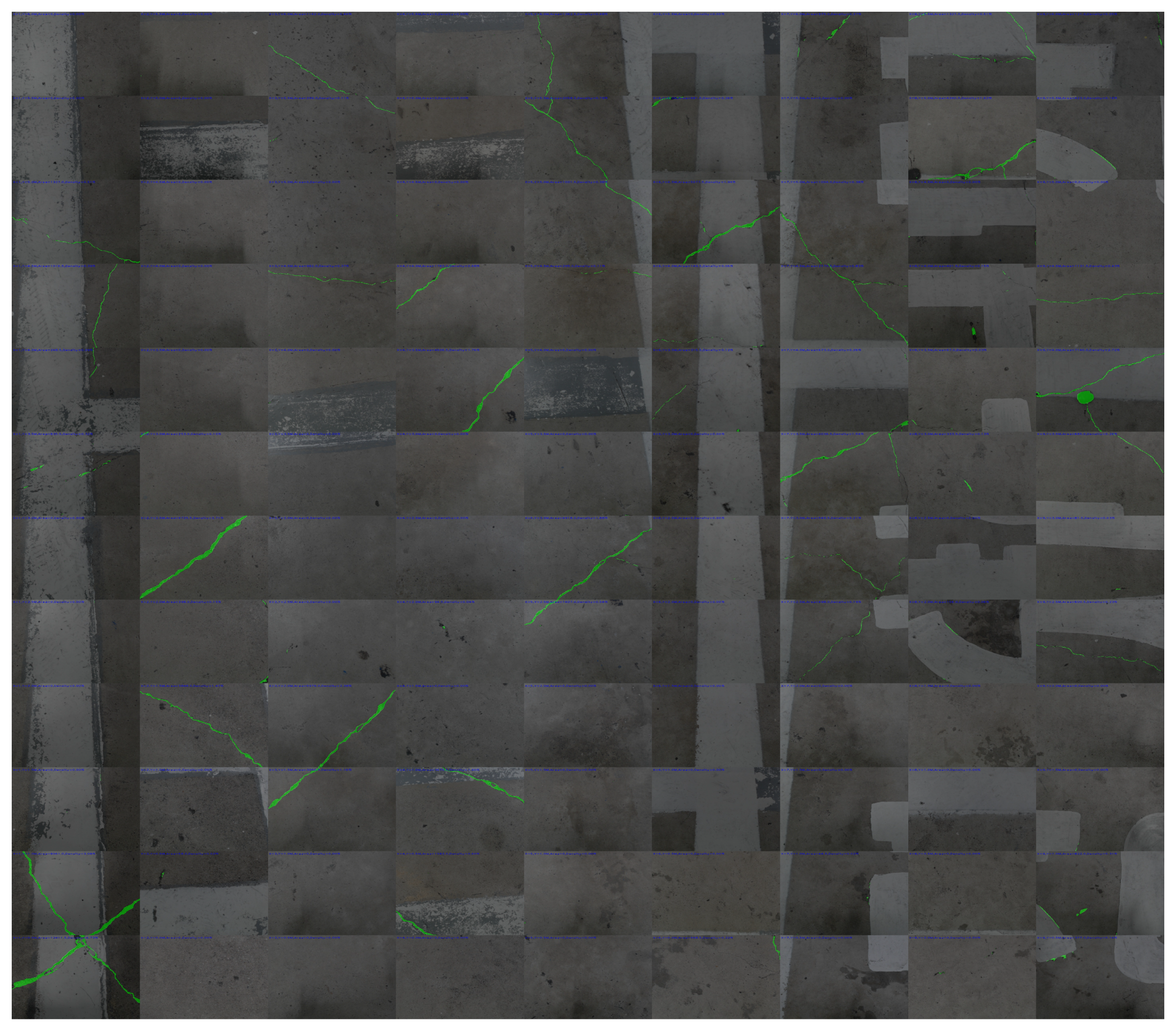
Figure 18.
Stitched image collected from the outdoor.
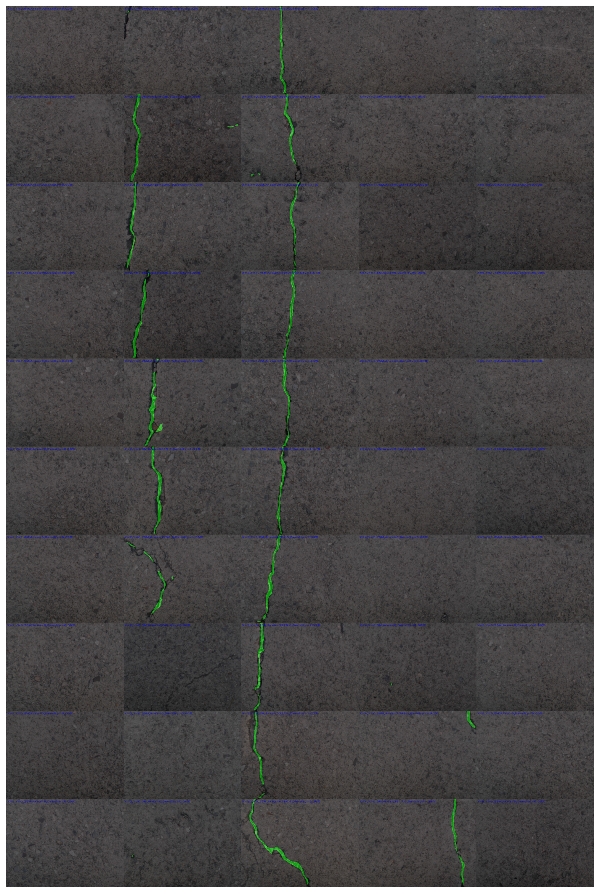
Figure 19.
Illustration of the severity of the cracks in the outdoor grid.
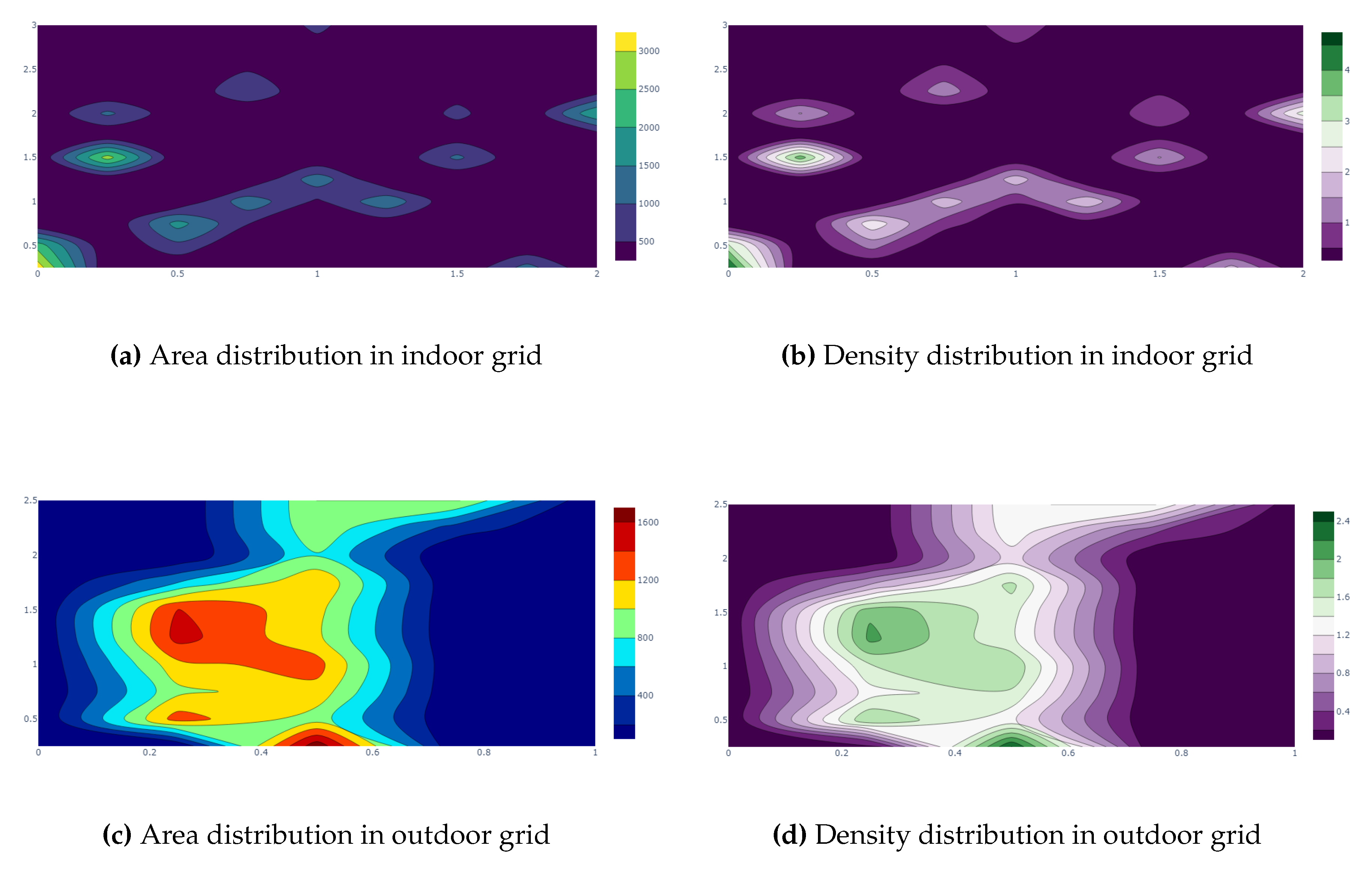

Table 1.
Summary of robotic platforms for crack inspection.
| Researchers | Inspected Structure | Robot Platform | Deep Learning | Remarks |
| Yu et al.[19] | Concrete Tunnel | Mobile robot | No | Images were collected by the robotic system. An image processing algorithm was utilized in an external computer for detecting cracks and crack information. |
| Oyekola et al.[20] | Concrete Tank | Mobile robot | No | Images were collected by the robotic system. A threshold-based algorithm was used in another computer for detecting the cracks. No postprocessing techniques were applied for obtaining geometrical information about the cracks. |
| Li et al.[21] | Concrete pavement | Guimi robot co ltd. | No | Detected crack using an unsupervised learning algorithm named MFCD. Detection was not performed in onboard ocmputer |
| La et al.[22] | Steel bridge | Wall climbing robot | No | Images were collected and passed to the ground station in real-time. Cracks were detected using the Hessian-matrix algorithm. Images were stitched and reconstructed to 3d for giving a visual idea. |
| La et al.[23] | Bridge deck | Seekur robot | No | Combined visual sensor and NDE sensors for crack inspection. Presented stitched images after crack detection and delamination map. |
| Hendrik et al.[24] | Concrete sweres | ANYmal (legged robot) | Yes (Machine learning) | Tactile sensory system were used to collect time series signals from the footstep of ANYmal and Support Vector Machine (SVM) were used to classify good, satisfactory, fair, critical, failure types or cracks. |
| Le et al.[25] | Concrete pipe | Mobile robot | Yes (Machine Learning) | Data from the camera and other sensors were fused to classify using SVM for detecting cracks. |
| Lei et al.[26] | Concrete Pavement | UAV | Yes (Machine Learning) | Images were collected by a CCD camera and the cracks were detected in the onboard computer of the UAV by SVM. The crack parameters were also computed. |
| Pan et al.[27] | Asphalt pavement | UAV | Yes (Machine learning) | Colected images using the UAV and the cracks were detected using Random Forest (RF), SVM, Artificial Neural Network (ANN) models. |
| Montero et al.[28] | Concrete Tunnel | Mobile robot | Yes | Collected RGB images using a camera and ultrasound data by an ultrasonic sensor. The data were passed to another computer for processing. A CNN model was used for detecting cracks from the images and a traditional method was used for estimating crack depth from the ultrasonic data. |
| Li et al.[29] | Concrete Bridge | Flying robot | Yes | A deep learning model was developed named Adanet for detecting cracks and 3d metrics were also reconstructed for getting the crack location and severity information. A dataset named Concrete Structure spalling and Cracking (CSSC) was also developed by this system. |
| Gui et al.[30] | Airport pavement | ARIR robot | Yes | Both surface and subsurface data were collected by a camera and GPR interfaced into the robotic system. An intensity-based algorithm and voting-based CNN were applied for processing image and GPR data. A large-scale stitched image was presented to visualize the cracks. |
| Ramalingam et al.[31] | Concrete pavement | Panthera robot | Yes | A SegNet-based model was developed to detect cracks and garbage. The system detects cracks on the onboard computer (Nvidia Jetson nano). A Mobile Mapping System was also utilized to localize the cracks. |
| He et al.[32] | Concrete Bridge | USV | Yes | A USV was applied to detect cracks in the bottom of a concrete bridge. The system detects cracks on the onboard computer (Intel NUC Mini PC) using cenWholeNet from the RGB and Lidar data. The results are then passed to the ground station in real-time. |
| Yang et al.[33] | Concrete wall | Climbing robot | Yes | A network named InspectionNet was used for detecting the cracks from the RGB-D camera on the onboard computer (Intel Nuc Mini PC) of the robotic system. A map-fusion module was also proposed to highlight the cracks. |
| Yuan et al.[34] | Reinforced concrete | Mobile robot | Yes | This robotic system used the stereo camera for collecting pictures and utilized a Mask RCNN model on the onboard computer (Nvidia Jetson nano) to detect cracks. A UI was also developed which controls the robot and receives data using WebSocket protocol. A 3d point cloud was reconstructed from the actual size of the cracks. |
Table 2.
AMSEL robot specifications.
| Parameter | Dimension | Unit |
| AMSEL Height | 21 | cm |
| AMSEL Width | 48.5 | cm |
| AMSEL Length (with sensor frame) | 91 | cm |
| AMSEL Length (without sensor frame) | 74 | cm |
| Sensor frame height | 35.3 | cm |
| Sensor frame length | 17 | cm |
| Sensor frame width | 36 | cm |
| Wheel numbers | 4 | - |
| Wheel radius | 13.25 | cm |
| Continuous driving time | >4 | hrs |
| Power source | Lipo battery | 22V |
| Sensor | RGB camera, vibration sensor | - |
Table 3.
RCDNet model performance in both train and test set
| Accuracy (%) | Dice Coefficient (%) | IoU (%) | Dice Loss(%) | |
|---|---|---|---|---|
| Train set | 96.35 | 97.40 | 97.35 | 0.0180 |
| Test set | 96.29 | 97.33 | 96.90 | 0.0214 |
Table 4.
Assessing severity of road cracks.
| Measurements (M) | Severity | Limit |
| Area (mm) | Fair | M<0.4% |
| Poor | 0.4% ≤ M<1 % | |
| Severe | M>1 % |
Table 5.
Comparison between the manually measured and digitally measured crack size indoor.
| Picture | Number of cracks | Manual length | Manual maximum width | No of cracks after prediction | Digital Length | Digital Maximum Width | Area | Density | Severity |
| 1.jpg | 1 | 227mm | 10mm | 1 | 227.45mm | 8.93mm | 1039.75mm2 | 1.44%. | Severe |
| 2.jpg | 2 | 72mm, 187mm | 3mm, 7mm | 2 | 72.04mm, 178.75mm | 2.82mm, 7.52mm | 484.675mm2 | 0.67%. | Poor |
| 3.jpg | 1 | 302mm | 17mm | 1 | 295.91mm | 15.97mm | 2123.575mm2 | 2.94%. | Severe |
| 4.jpg | 1 | 150mm | 5mm | 1 | 157.67mm | 5.11mm | 318.66mm2 | 0.44%. | Poor |
| 5.jpg | Web crack | - | - | Web crack | - | - | 4330.93mm2 | 6%. | Severe |
| 6.jpg | 1 | 240mm | 5mm | 1 | 232.56mm | 5.64mm | 344.98mm2 | 0.47%. | Poor |
| 7.jpg | 1 | 325mm | 8mm | 1 | 312.24mm | 7.82mm | 545.32mm2 | 0.83%. | Poor |
| 8.jpg | Web crack | - | - | Web crack | -mm | - | 599.83mm2 | 0.88%. | Poor |
| 9.jpg | 1 | 302mm | 9mm | 1 | 302mm | 8mm | 1227.775mm2 | 1.70%. | Severe |
| 10.jpg | 1 | 200mm | 3mm | 1 | 192.28mm | 2.82mm | 200.33mm2 | 0.32%. | Fair |
Table 6.
Comparison between the manually measured and digitally measured crack size outdoor.
| Picture | Number of cracks | Manual length | Manual maximum width | No of cracks after prediction | Digital Length | Digital Maximum Width | Area | Density | Severity |
| 11.jpg | 1 | 232mm | 8mm | 1 | 224.87mm | 7.52mm | 1144.09mm2 | 1.59%. | Severe |
| 12.jpg | 1 | 307mm | 10mm | 1 | 300.86mm | 10.81mm | 1912.665mm2 | 2.65%. | Severe |
| 13.jpg | Web crack | - | - | Web crack | - | - | 2747.5mm2 | 3.81%. | Severe |
| 14.jpg | Web crack | - | - | Web crack | - | - | 3699.37mm2 | 5.12%. | Severe |
| 15.jpg | 1 | 351mm | 17mm | 1 | 341.33mm | 15.81mm | 1713.26mm2 | 2.37%. | Severe |
| 16.jpg | 1 | 240mm | 9mm | 1 | 225.67mm | 18.33mm | 1712.32mm2 | 2.37%. | Severe |
| 17.jpg | 2 | 312mm, 255mm | 9mm,6mm | 2 | 305.15mm, 238.87mm | 8mm, 6.11mm | 2575.13mm2 | 3.56%. | Severe |
| 18.jpg | 1 | 323mm | 10mm | 1 | 306.92mm | 10.81mm | 1841.572mm2 | 2.55%. | Severe |
| 19.jpg | 2 | 268mm, 98mm | 8mm,18mm | 2 | 253mm, 63.92mm | 8.46mm, 17.86mm | 1487.54mm2 | 2.06%. | Severe |
| 20.jpg | 1 | 230mm | 9mm | 1 | 224.43mm | 10mm | 1179.81mm2 | 1.63%. | Severe |
Table 7.
Statistics of the detected cracks for indoor area shown in Figure 17.
Table 7.
Statistics of the detected cracks for indoor area shown in Figure 17.
| Number of cracks | Maximum Area | Minimum Area | Total Area | Total Density |
| 43 | 3841.995mm2, Loc. (x=0m, y=0.25m) | 38.305mm2 ,Loc. (x=2m, y=3m) | 22617.69mm2 | 0.38% |
Table 8.
Statistics of the detected cracks for the outdoor area shown in Figure 18.
Table 8.
Statistics of the detected cracks for the outdoor area shown in Figure 18.
| Number of cracks | Maximum Area | Minimum Area | Total Area | Total Density |
| 18 | 1741.35mm2, Loc. (x=0.5m, y=0.25m) | 308.2025mm2 ,Loc. (x=0.75m, y=0.5m) | 15231.88mm2 | 0.68% |
Disclaimer/Publisher’s Note: The statements, opinions and data contained in all publications are solely those of the individual author(s) and contributor(s) and not of MDPI and/or the editor(s). MDPI and/or the editor(s) disclaim responsibility for any injury to people or property resulting from any ideas, methods, instructions or products referred to in the content. |
© 2023 by the authors. Licensee MDPI, Basel, Switzerland. This article is an open access article distributed under the terms and conditions of the Creative Commons Attribution (CC BY) license (http://creativecommons.org/licenses/by/4.0/).
Copyright: This open access article is published under a Creative Commons CC BY 4.0 license, which permit the free download, distribution, and reuse, provided that the author and preprint are cited in any reuse.


