Submitted:
06 June 2023
Posted:
07 June 2023
You are already at the latest version
Abstract
The study of fractures in the subsurface is very important in unconventional reservoirs since they are the main conduits for hydrocarbon flow. For this reason, a variety of equivalent medium theories have been proposed for the estimation of fracture and fluid properties within reservoir rocks. We experimentally investigated the feasibility of applying the Galvin model in fractured tight stones. For this proposal, three artificial fractured tight sandstone samples with the same background porosity (11.7% ± 1.2%) but different fracture densities of 0.00, 0.0312, and 0.0624 were manufactured. The fracture thickness was 0.06 mm and the fracture diameter was 3 mm in all the fractured samples. Ultrasonic P- and S-wave velocities were measured at 0.5 MHz in a laboratory setting in dry and water-saturated conditions in directions at 0°, 45°, and 90° to the fracture normal. The results were compared with theoretical predictions of the Galvin model. The comparison showed that model predictions significantly underestimated P- and S- wave velocities as well as P-wave anisotropy in water-saturated conditions, but overestimated P-wave anisotropy in dry conditions. By analyzing the differences between the measured results and theoretical predictions, we modified the Galvin model by adding the squirt flow mechanism to it and used the Thomsen model to obtain the elastic moduli in high- and low-frequency limits. The modified model predictions showed good fits with the measured results.
Keywords:
Artificial fractured tight stones
; equivalent medium theories
; rock physics
; experimental validation
; anisotropy
1. Introduction
In unconventional reservoirs with low matrix permeability, fractures can be the main conduits for the flow of pore fluids. Fracture detection and characterization are very important in the context of oil/gas exploration and production. As a result, analyses of fracture physical characteristics (scale, aperture, orientation) and their influences on seismic propagation have attached considerable interest in academia and industry.
Equivalent medium theories have been used to bridge the rock physics relationships between rock, fracture, and fluid properties to seismic velocity, attenuation, and anisotropy. Traditionally, the theories of Schoenberg (1988) [1,2], Thomsen (1995) [3], and Gurevich (2003) [4] have been applied. However, these models have strict frequency limitations because of the assumptions in their derivation processes. The model of Schoenberg (1988) is usually referred to as a linear-slip model and is limited to a high-frequency regime wherein fluid is isolated in fractures, whereas the Gurevich model is limited to a low-frequency regime with fluid allowed to flow between fractures and quant pores. The Thomsen model provides different expressions in low- and high-frequency regimes, respectively. These three models neglect the dispersion effect and cannot be used to obtain the frequency-dependent moduli of fractured rocks. Brajanovski et al. (2005) extended the Gurevich model and derived an analytical solution for P-wave dispersion [5]. Galvin and Gurevich provided a unified model by branching function approximation [6,7]. This approximation has similar behavior compared to asymptotic analytical solutions at low and high frequencies and satisfies causality, turning out to be very accurate and useful. We refer to the Galvin and Gurevich (2015) model as the Galvin model.
Validation of these theoretical models through well-designed laboratory experiments is desirable. Unfortunately, the fractures are unknown and cannot be quantitatively controlled in natural rocks. Thus, artificial sandstones with controlled fractures are frequently used to study seismic wave propagation in fractured rocks by conducting laboratory experiments. Rathor (1995) provided P- and S-wave velocity results in artificial fractured sandstones bounded by epoxy [8], and the data set confirmed the nature of seismic anisotropy in porous rocks with aligned penny-shaped fractures. The measured results were compared with predictions of the Hudson model and Thomsen model, and the results demonstrated significant effects of fluid flow on seismic velocity and anisotropy. Tillotson (2012, 2014) investigated the feasibility of the Chapman model in predicting seismic velocity and anisotropy in silica-cemented artificial rocks [9,10]. Ding (2017, 2018) experimentally investigated the effects of fracture density and scale on seismic velocity anisotropy [11,12]; the results were compared with those of the Chapman model and good fits were found between the measured data and theoretical predictions. However, as previous experimental studies based on artificial fractured sandstones are often conducted in the high-porosity range (>29%), there are, so far, few experimental studies that address the reliability of equivalent medium theories of low-porosity fractured rocks, despite the fact that unconventional reservoirs are usually characterized by low porosity and low permeability.
In this work, we aimed to investigate the application of the Galvin model for low-porosity artificial fractured sandstones. We constructed three artificial fractured sandstone samples with the same background matrix porosity (11.7% ± 1.2%) but different fracture densities (0%, 3.12%, and 6.24%). The P- and S-wave velocities as well as the anisotropic parameters were measured experimentally and compared with the predictions of the Galvin model. The differences between the measured results and theoretical predictions were analyzed, based on which some modifications were made to the Galvin model.
2. Theoretical Background
The Galvin model seeks to model frequency-dependent elastic moduli in fractured porous rocks [7]. The elastic stiffness tensor given by Galvin (2015) is of the following form:
where and are the stiffness tensor in the high- and low-frequency limits, which can be obtained by the linear-slip theory and the Gurevich (2003) model, respectively. and are parameters that shape the dispersion and attenuation curves of the elastic coefficient:
where and are the P-wave modulus of the fractured rock in the fracture normal direction in the low- and high-frequency limits. For sparsely distributed penny-shaped cracks, the expressions of T and G are of the following form:
where and are the P-wave modulus of fluid saturated and dry background matrix, respectively; is the matrix permeability; is Biot’s coefficient of the matrix, with being the bulk modulus of the dry background matrix and that of the solid grains composing the matrix.
is Biot’s background matrix modulus, with being the fluid bulk modulus and the porosity of the background. is the shear modulus of the dry background matrix. is the fracture radius and is the fracture density:
In dry conditions, and are equal and the Galvin model returns to linear-slip model in which the elastic compliance tensor of the fractured medium is of the following form:
where is the dry compliance tensor of the background matrix. is the excess compliance tensor associated with the fractures and can be expressed in the following form:
where and denote the so-called normal and shear excess compliances caused by the presence of fractures, respectively.
In fluid-saturated conditions, high-frequency-limit fluid does not have enough time to flow between pore space and fractures; this regime is called ‘unrelaxed’ by Mavko and Jizba (1991). In the Galvin model, the compliance tensor of fractured rocks in the high-frequency limit was calculated by linear-slip model by the following form:
where is the inverse of the fluid-saturated matrix stiffness tensor which is given by the Gassmann equation and dry moduli of the background matrix.
At the low-frequency range, fluid has enough time to flow between pores and fractures. In the Gurevich (2003) model, fluid-saturated moduli can be obtained by combining the linear-slip model and the anisotropic Gassmann equation:
where is the stiffness tensor of the fractured rock and is Biot’s coefficient, which takes the following form:
and M is Biot’s modulus:
where is the overall porosity and was defined as follows:
In laboratory experiments through artificial fractured sandstones, the background matrix of samples usually exhibited some extent of anisotropy. To model the anisotropy caused by fractures, the anisotropy of the background matrix must be taken into account first of all. Tillotson (2014) modified Chapman (2003) model to account for background matrix anisotropy when modeling fracture-induced anisotropy. In the approach of Tillotson (2014), the isotropic background matrix moduli assumed by Chapman model was replaced by the measured anisotropic background moduli, which is formed by measured velocities and bulk densities of the blank sample (without fractures). Similarly, in order to take account the anisotropy in background matrix, we replaced the isotropic dry background compliance tensor assumed by Galvin model in equation (6) with measured anisotropic compliance tensor of dry background matrix , which can be obtained by , , , and and bulk density in
sample 1# using the equations of Mavko et al. (1998) [13].
3. Sample Preparation and Velocity Measurement
The method of Ding (2014a) was adapted to construct artificial tight sandstones with similar mineral components [14], pore structures, and cementation to natural rocks. In this method, powders of silica sand, feldspar, and kaolinite were mixed in a ball mill for 24 h to ensure homogeneity. Then, these mineral powders were mixed with sodium silicate, and the mixture was poured into a mold layer by layer. To form the penny-shaped “meso-scale” fractures, touch paper discs were spread on the surface of the mineral powder mixtures when layering the mixture in the mold. Touch paper is a special kind of paper which has been soaked in saltpeter. At high temperature touch paper would be decomposed into gas and leave nearly no remain. Thereafter, compression was applied to compact the mineral grains. In this way, a block was formed, and consolidated sodium silicate gave the block its initial mechanical strength. The block was then sintered in a muffle oven at 900 °C. In the sintering process, the touch paper discs decomposed into gas, leaving penny-shaped voids to simulate these fractures.
Three low-porosity artificial rocks with different fracture densities (0, 0.0312, and 0.0624) were fabricated (Figure 1a). Each rock was made in exactly the same way except for the introduction of fractures. Fracture density is controlled by setting the number of fractures per layer (Table 1). The penny-shaped fractures were distributed parallelly in fractured samples with a 3 mm fracture diameter and 0.06 mm fracture aperture (Figure 1b). All samples were ground into sexangular prisms to make it possible to conduct ultrasonic velocity measurements at 0°, 45°, and 90° to the fracture normal (Figure 1c).
Table 1 and Table 2 show the main parameters of the three synthetic rocks. The porosity was measured using helium porosimetry. In the fractured samples, the background porosities were calculated by subtracting fracture-induced porosity from the total porosity of the sample. The background porosity difference between the three samples was less than 1.2%; this was caused by some inevitable tiny errors during the manufacturing process.
Figure 2 shows the SEM image of the artificial rock, pore structure, and parallelly distributed fractures with controlled geometry.
P- and S-wave velocity measurements were conducted on an ultrasonic bench-top pulse transmission system at room temperature and atmospheric pressure for dry and water-saturated conditions. The measurement was based on the test standard DZ/T0276.24-2015. The central frequency of P and S transducers was 0.5 MHz and the time sampling interval was 0.04 μs for both P- and S-wave signals. The measurement error was about 0.5% for P-wave velocity and 0.8% for S-wave velocity. Water saturation was obtained by immersing the samples in a water-filled container, which was placed in a sealed bin to extract the air. To ensure full water saturation, the saturation rate was calculated as follows:
where and are the wet and dry masses of the sample, respectively, and are the volume and helium-porosimetry-measured porosity of the sample, respectively, and is the bulk density of water.
P- and S-wave velocities were measured in three directions at 0°, 45°, and 90° to the fracture normal. In each direction, both S1 and S2 velocities were measured for polarization parallel (S1) and perpendicular (S2) to the fractures by rotating the transducers.
Through a numerical modeling experiment, Dellinger and Vernik (1994) indicated that for wave propagation parallel or perpendicular to the layering (or in this case fractures), a true phase velocity is measured in laboratory ultrasonic experiments. However, a wavefront propagating at 45° to the fracture normal can suffer a lateral translation. If the lateral translation suffered by the wave is greater than the radius of the receiving transducer, then a group velocity is measured instead of a phase velocity. Equations in Dellinger & Vernik (1994) was used to calculate the lateral translations at 45°, and the results show that the value was within 8.03 mm for all measurements, smaller than our transducer radius (12.5 mm). Therefore, we concluded that we measured the phase velocity for both P- and S-waves in three directions. A similar conclusion was reached by Ding (2018) using the same experimental setup as that used in this study.
4. Results
Figures 3a, 4a and 5a show P-wave velocity variation with the propagation angle in three samples. The P-wave velocity was the fastest in the 90° direction and the slowest in the 0° direction in all samples.
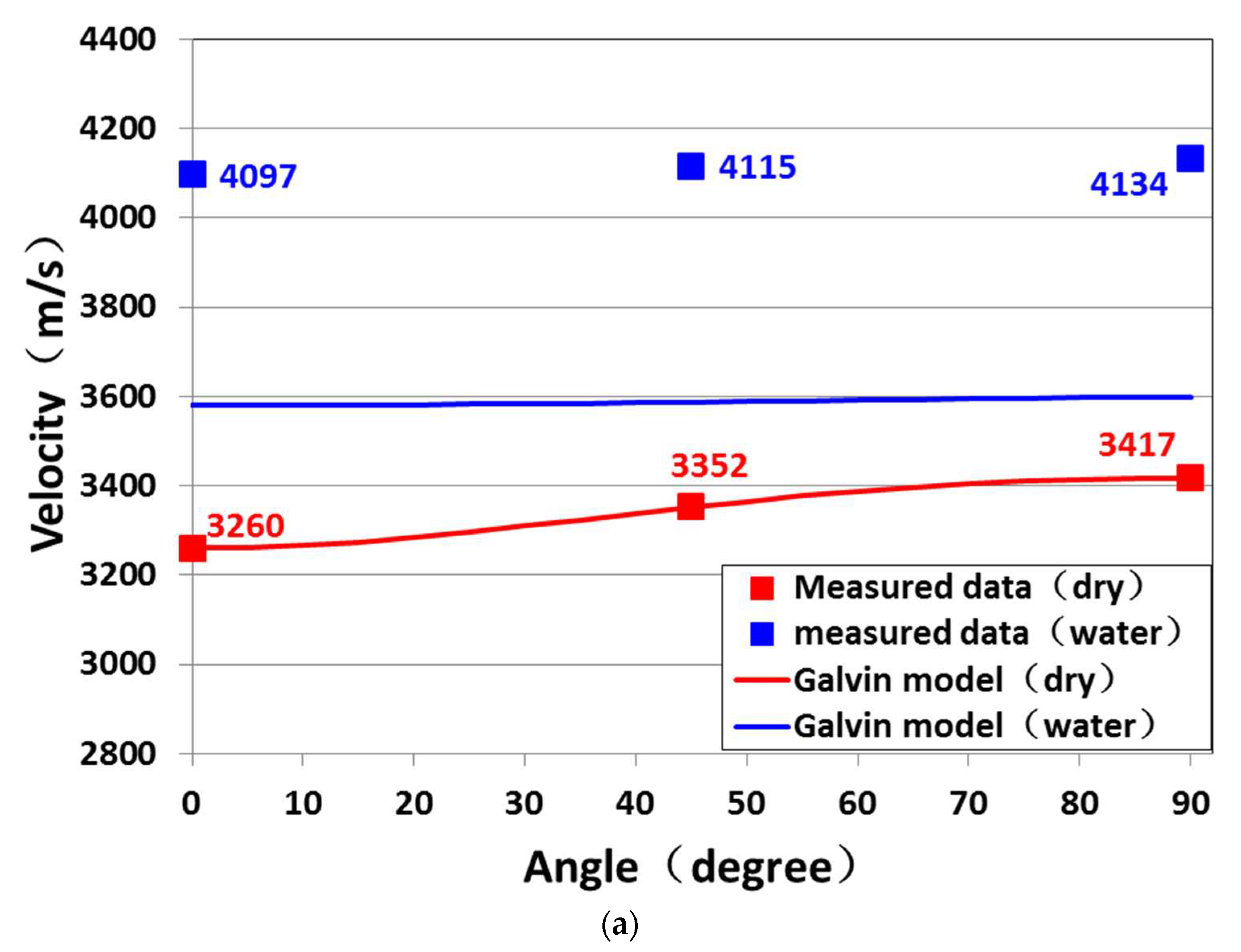
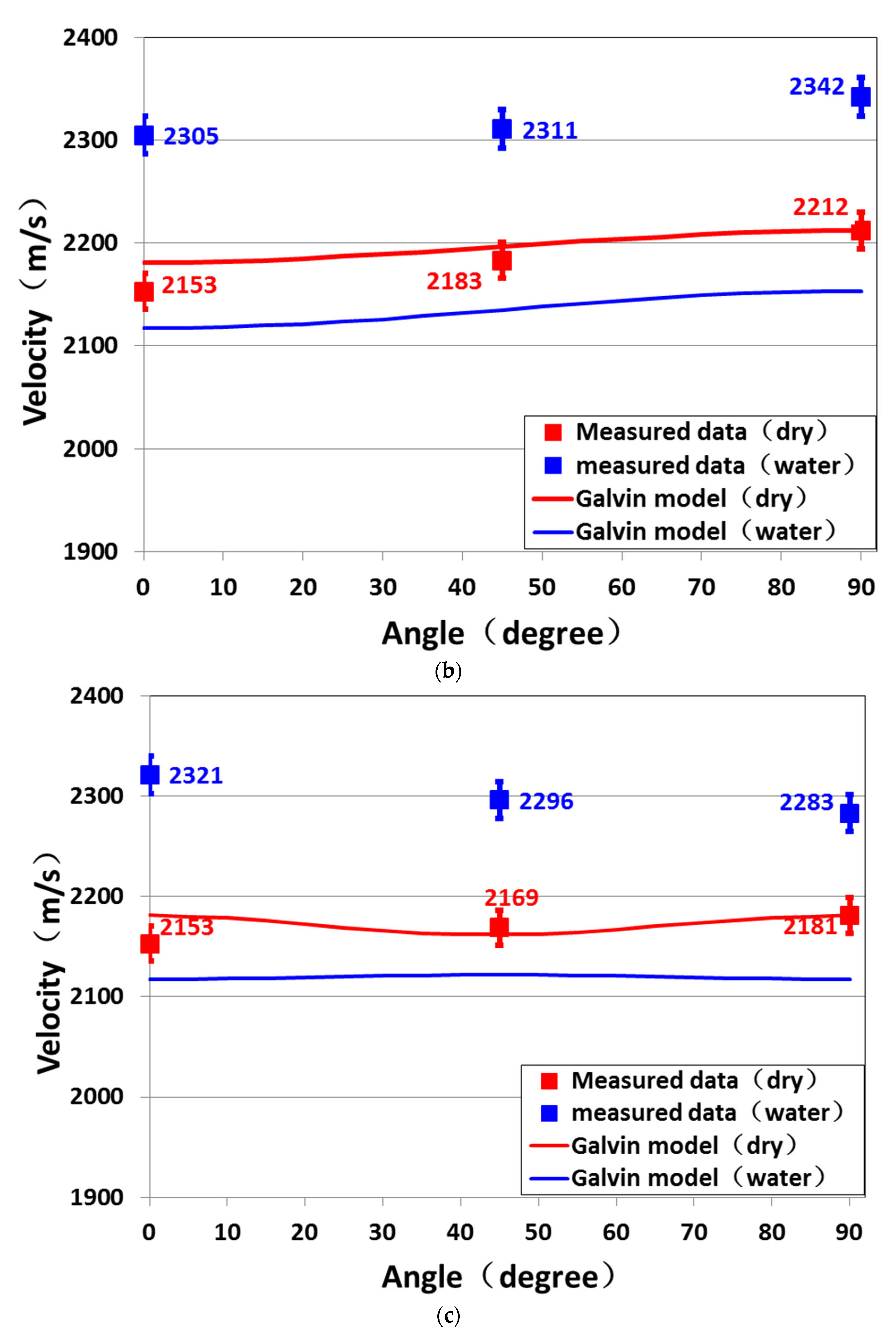
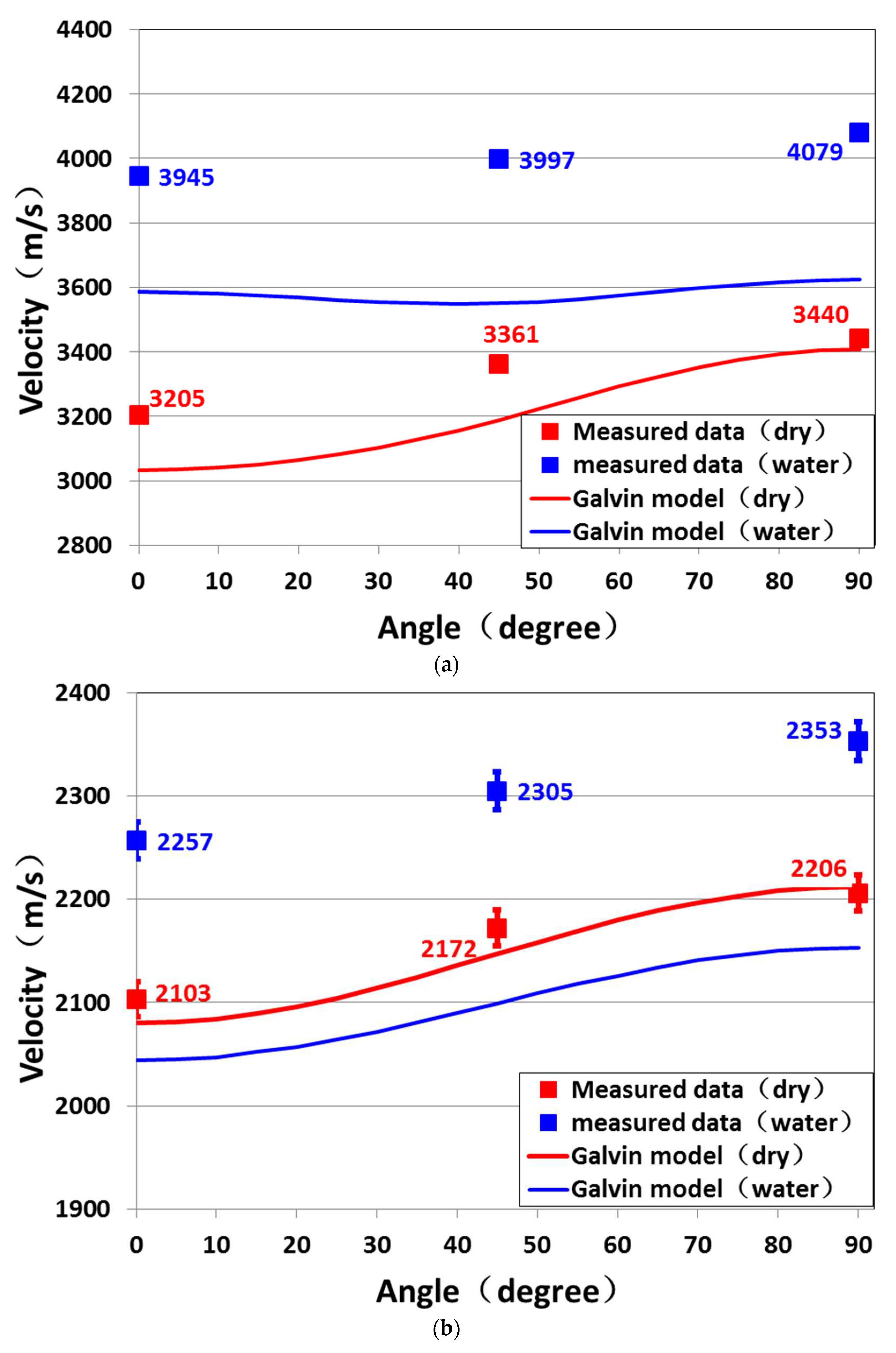
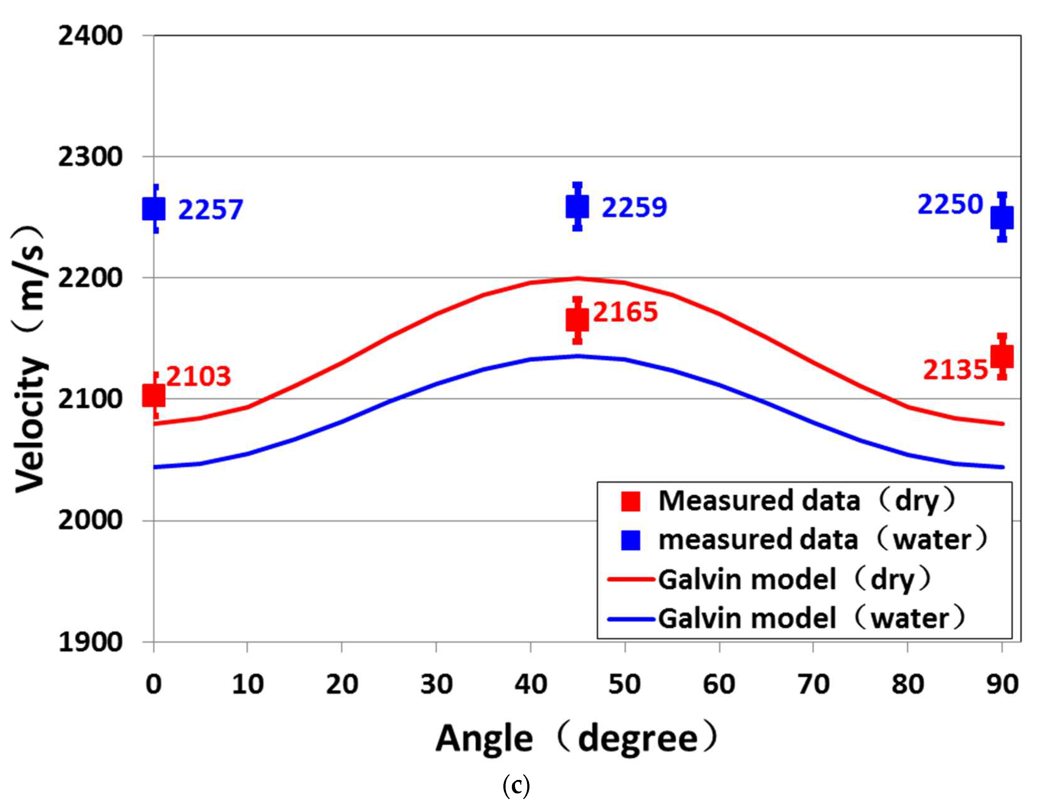
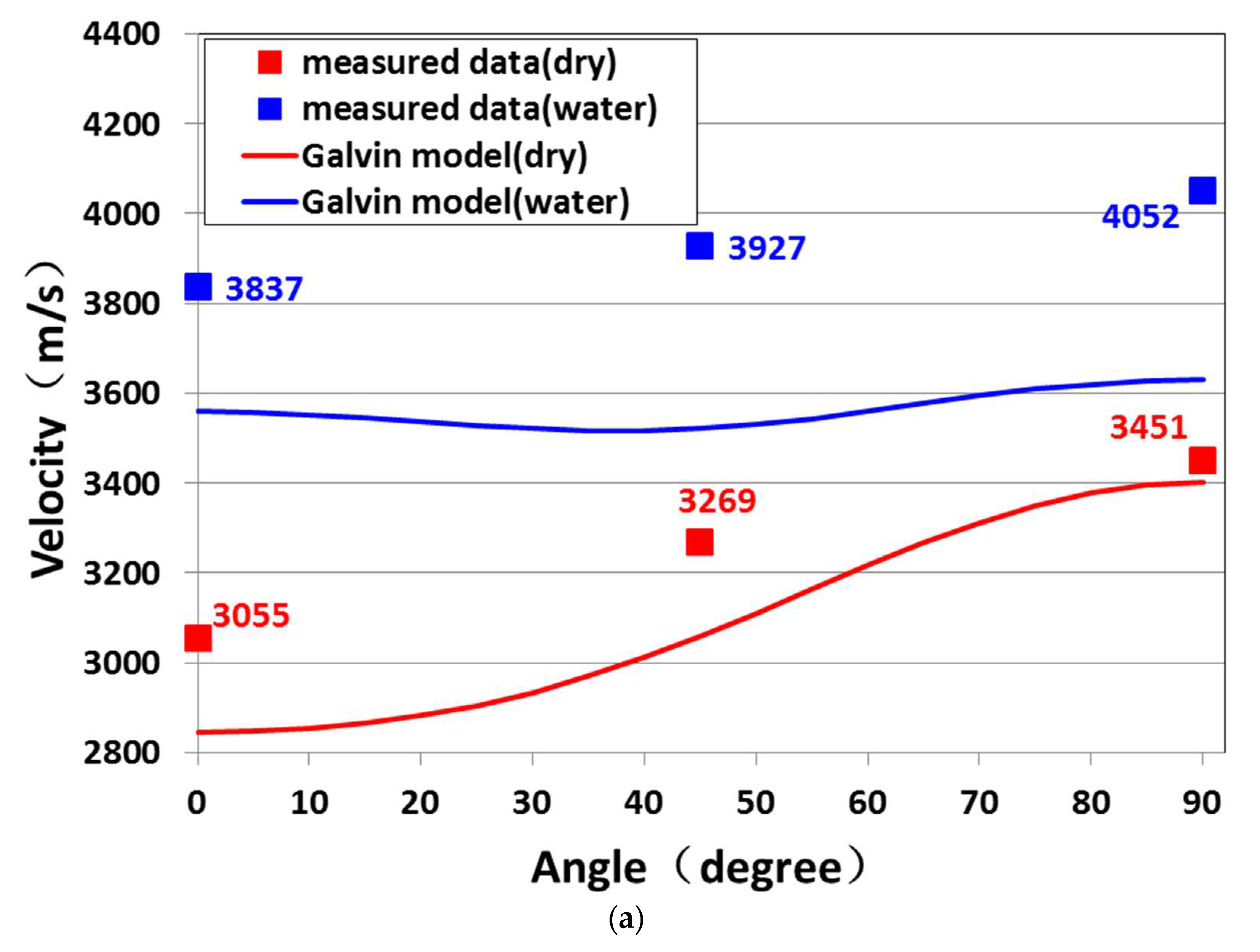
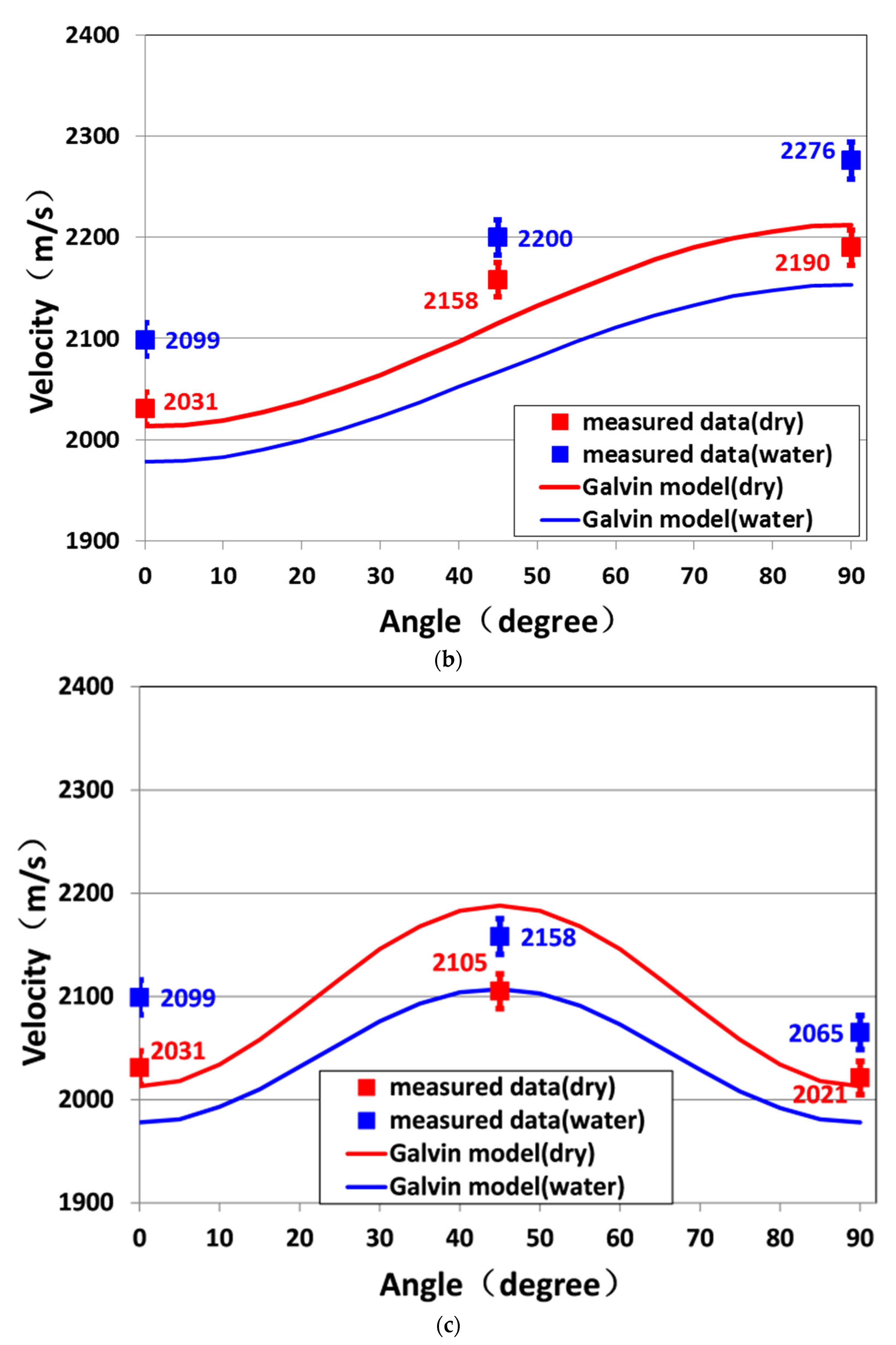
Figure 3.
Measured velocity and theoretical predictions of the Galvin model for the 1# sample (fracture density 0). (a) P-wave (P-wave velocity measurement error is smaller than the size of labels); (b) SH-wave; and (c) SV-wave.
Figure 3.
Measured velocity and theoretical predictions of the Galvin model for the 1# sample (fracture density 0). (a) P-wave (P-wave velocity measurement error is smaller than the size of labels); (b) SH-wave; and (c) SV-wave.
Figure 4.
Measured velocity and theoretical predictions of the Galvin model for the 2# sample (fracture density 0.0312). (a) P-wave (P-wave velocity measurement error is smaller than the size of labels); (b) SH-wave; and (c) SV-wave.
Figure 4.
Measured velocity and theoretical predictions of the Galvin model for the 2# sample (fracture density 0.0312). (a) P-wave (P-wave velocity measurement error is smaller than the size of labels); (b) SH-wave; and (c) SV-wave.
Figure 5.
Measured velocity and theoretical predictions of the Galvin model for the 3# sample (fracture density 0.0624). (a) P-wave (P-wave velocity measurement error is smaller than the size of labels); (b) SH-wave; and (c) SV-wave.
Figure 5.
Measured velocity and theoretical predictions of the Galvin model for the 3# sample (fracture density 0.0624). (a) P-wave (P-wave velocity measurement error is smaller than the size of labels); (b) SH-wave; and (c) SV-wave.
The P-wave velocity variation with the direction in the 1# sample indicated some anisotropy in the background matrix in all samples; this is due to layering in the construction process and frequently encountered in previous experimental studies [9,10,11,12]. For P-wave propagation at oblique (45°) and perpendicular (0°) angles, in fractured samples, the aligned fractures can increase the compliance of rocks and reduce P-wave velocity. In the 90° direction, the measured P-wave velocity in samples 2# and 3# was higher than 1# in the dry condition, and lower than 1# in the water-saturated condition. Theoretical and experimental studies indicated that in the 90° direction [12], P- and SH-wave velocity only decrease very slightly with the increase of fracture density, because fractures are hard to compress in this direction. Therefore, the difference of the measured P-wave between different fracture density samples in the 90° direction is mainly due to both the background matrix property differences within the three samples and the velocity measurement error.
In dry conditions, theoretical predictions fit well with the measured P-wave in the 90° direction. However, in fractured samples (2# and 3#), theoretical predictions underestimated the P-wave velocity at 45° and 0°, indicating the predicted P-wave anisotropy was larger than the measured data. In water-saturated conditions, predicted P-wave velocities were well below the measured results. In the Galvin (2015) model, the fluid-saturated background matrix modulus is calculated by Gassmann theory. The results for the 1# sample indicated that Gassmann theory significantly underestimated P-wave velocity in the water-saturated background matrix in the three samples. Meanwhile, the measured P-wave velocity showed 2θ periodicity while the predicted P-wave velocity showed 4θ in the propagation direction.
Figures 3b, 4b and 5b show comparisons of the SH-wave velocities with measured data versus the propagation direction angle in samples with different fracture densities. In dry conditions, the predicted SH-wave velocity qualitatively fit the measured data, and some underestimation was found in the 45° and 0° directions. In water saturation, for sample 1#, the measured SH-wave velocity was higher than in dry conditions, while in theoretical prediction water saturation can reduce SH-wave velocity from dry conditions. The Gassmann theory assumes that water saturation does not influence shear modulus, . Since water saturation can increase the bulk density but has no effect on shear modulus in theoretical prediction, the predicted water-saturated SH- and SV-wave velocities were lower than those in dry conditions. The results of SH-wave velocity in sample 1# indicated that water saturation can greatly increase the shear modulus in the background matrix. Regardless, in water saturation, the predicted SH-wave velocity qualitatively fit the measured data. In fractured samples, dry SV-wave velocity was slightly underestimated in the 0° and 90° directions and significantly overestimated in the 45° direction (Figures 3c, 4c and 5c). The predicted SV-wave velocity exhibited greater variation with propagation angle than the measured data in both dry and water-saturated conditions.
Figure 6a shows a comparison of the P-wave anisotropy parameter ε between the measured data and theoretical prediction in dry and water-saturated conditions. P-wave anisotropy was higher in samples with larger fracture densities because the presence of penny-shaped fractures increases the compliance of samples in perpendicular directions to a much larger extent than in parallel directions. The predicted P-wave anisotropy was higher than that measured in dry conditions and lower than the measured data in water-saturated conditions in fractured samples. The predicted S-wave anisotropy was slightly higher than the measured data in both dry and water-saturated conditions (Figure 6b).
5. Discussion
We tested our experimental results against predictions of the Galvin model from an experimental point of view. Predicted P- and S-wave velocity in water-saturated conditions were well below the measured data. The Galvin model uses Gassmann theory to calculate the fluid-saturated background matrix modulus. However, the Gassmann theory is valid only at sufficiently low frequencies because it assumes that the induced pore pressure is equilibrated throughout the pore space (i.e., there is sufficient time for the pore fluid to flow and eliminate wave-induced pore pressure gradients). The experimental frequency (0.5 MHz) was higher than the low-frequency range assumed by Gassmann theory, so pore pressure was not equilibrated throughout the pore space. This acts to ‘stiffen’ the rock and make P- and S-wave velocity higher than in the theoretical prediction. Similar observations can be found in ultrasonic experimental studies of tight stones, and Li (2018) indicated the dispersion effect caused by local fluid flow between pores and microcracks makes measured velocity higher than in Gassmann-theory-based prediction.
Considering the differences between the measured data and theoretical predictions, several modifications were made to the Galvin model: (i) the Dvorkin (1995) squirt flow model was used to replace the Gassmann model to calculate the fluid-saturated background matrix modulus [17]. The parameter Z in the Dvorkin model was found by matching the measured P-wave velocity and theoretical prediction. (ii) The elastic moduli of the fractured rocks in the low- and high-frequency limits were obtained by the Thomsen model instead of the linear-slip model or the Gurevich (2003) model. Figure 7, Figure 8 and Figure 9 show comparisons of the measured P-, SH-, and SV-wave velocities with the prediction of the Galvin model and the modified Galvin model. In water saturation, predicted P-, SH-, and SV-wave velocities in the modified model were significantly higher than that in the Galvin model, indicating that squirt flow can increase both bulk and shear moduli. Predicted P-wave velocities of the modified model were very close to measured data. In the modified model prediction, SH- and SV-wave velocity in water saturation were higher than in dry conditions; this is in agreement with measured data but contradicts the Galvin model. However, the modified model predicted SH- and SV-wave velocities were still lower than the measured results in water-saturated conditions. For dry conditions, since the measured results of sample 1# were used as inputs in the Galvin model and modified Galvin model, both models yielded the same predictions of dry velocities of three modes of waves in 1#. In sample 2# and 3#, predictions of dry P- and SH-wave velocities between the Galvin model and the modified model were close to each other, but predictions of the SV-wave in the modified model exhibited smaller variations with propagation angle than the Galvin model and were qualitatively closer to the measured data.
Figure 10 shows comparisons of the measured P-wave anisotropy with the prediction of the Galvin model and the modified Galvin model. In water-saturated conditions, the predicted P-wave anisotropy of the modified model was higher than that of the Galvin model and close to the measured results; Meanwhile, S-wave anisotropy prediction in the modified model was slightly lower than the Galvin model. Whereas, in dry conditions, the modified model yielded nearly the same P-wave anisotropy and S-wave anisotropy as the Galvin model. In dry conditions, Galvin model prediction agreed with that of the linear-slip model, and the modified model prediction agreed with the Thomsen model. The linear-slip model and Thomsen model yielded nearly the same dry P- and S-wave anisotropy parameters. In water-saturated conditions, the modified model predicted larger P-wave anisotropy than the Galvin model. That is mainly because the predicted P-wave anisotropy of and of the modified model was higher than the Galvin model. Table 3 lists the predicted P-wave anisotropy parameter in and of the modified model and Galvin model in sample 2#. In the Galvin model, and were calculated by the linear-slip model and Gurevich (2003) model, respectively. In the modified model, the Thomsen model yielded higher P-wave anisotropy than the linear-slip and Gurevich (2003) models in high- and low-frequency limits, respectively.
In the modified model, the predicted P-wave anisotropy was close to that of the measured data in water-saturated conditions but significantly higher than measured in dry conditions. This might be due to the interaction between the fractures. In the Galvin model and the modified model, the interaction between fractures is neglected. For air saturation, the difference between fracture infill material (air) and background medium was large, and the interaction between fractures was strong. Numerical studies indicated that the interaction between fractures can reduce P- and S-wave anisotropy [18]. This gives rise to the overestimation of P-wave anisotropy in the modified model. For water saturation, the modulus difference between the fracture infill material (water) and the background medium was greatly reduced compared with the dry case, and the interaction between fractures was relatively weak. This resulted in a good fit between measured P-wave anisotropy and the prediction of the modified model.
6. Conclusions
Validating the theoretical models of seismic wave velocity, attenuation, and anisotropy in fractured rocks in a laboratory setting remains an important goal. Previous studies have been conducted in high-porosity ranges that represent very different physical properties compared with those of unconventional reservoirs. There is a lack of experimental validations of equivalent medium theories in fractured tight rocks. This study focused on investigating the feasibility of the Galvin model in low-porosity fractured rocks by observing P- and S-wave velocities and anisotropy in a set of low-porosity artificial fractured sandstones. Three samples with different fracture densities were used for laboratory ultrasonic measurements at 0.5 MHz while the samples were dry and water saturated. The measurements showed that the Galvin model significantly overestimated P- and S-wave velocities as well as P-wave anisotropy in water-saturated conditions. Based on the comparison between measured data and theoretical predictions, we modified the Galvin model by (1) using the Dvorkin (1995) squirt flow model to calculate the frequency-dependent moduli of the background matrix, thus adding a squirt flow effect into the Galvin model; and (2) using the Thomsen model to calculate the elastic moduli of the fractured rocks in low- and high-frequency limits.
In water saturation, predictions of the modified model fit well with the measured data. However, in dry conditions, the predicted P-wave anisotropy of the modified model was still significantly higher than the measured results. This might be due to the interaction between fractures, which acts to reduce overall anisotropy in dry conditions but has little effect on anisotropy in water-saturated conditions. Neither the Galvin model nor the modified model take the interaction between fractures into account. In both dry and water-saturated conditions, predicted S-wave anisotropy of the modified model was slightly higher than the measured results.
Author Contributions
sample manufacturing, ultrasonic measurement, data analysis, Zhang. Y.; Supervision: Di. B. All authors have read and agreed to the published version of the manuscript. All authors have read and agreed to the published version of the manuscript.
Funding
This research received no external funding.
Data Availability Statement
Not applicable.
Conflicts of Interest
The authors declare no conflict of interest.
References
- Schoenberg, M.; Douma, J. Elastic-wave propagation in media with parallel fractures and aligned cracks. Geophys. Prospect. 1988, 36, 571–590. [Google Scholar] [CrossRef]
- Schoenberg, M.; Sayers, C.M. Seismic anisotropy of fractured rock. Geophysics 1995, 60, 204–211. [Google Scholar] [CrossRef]
- Thomsen, L. Elastic anisotropy due to aligned cracks in porousrock. Geophysical Prospecting 1995, 43, pp. 805–829. [Google Scholar] [CrossRef]
- Gurevich, B. Elastic properties of saturated porous rocks with aligned fractures. J. Appl. Geophys. 2003, 54, 203–218. [Google Scholar] [CrossRef]
- Brajanovski, M.; Gurevich, B.; Schoenberg, M. A model for P-wave attenuation and dispersion in a porous medium permeated byaligned fractures. Geophysical Journal International 2005, 163(1), pp. 372–384. [CrossRef]
- Galvin, R.J.; Gurevich, B. Effective properties of a poroelastic medium containing a distribution of aligned cracks. J. Geophys. Res. 2009, 114. [Google Scholar] [CrossRef]
- Galvin, R.J.; Gurevich, B. Frequency-dependent anisotropy of porous rocks with aligned fractures. Geophys. Prospect. 2014, 63, 141–150. [Google Scholar] [CrossRef]
- Rathore J.S.; Fjaer .E.; Holt R.M. P- and S-wave anisotropy of a synthetic sandstone with controlled crack geometry. Geophysical Prospecting 1995, 43(6), pp. 711-728. [CrossRef]
- Tillotson, P.; Sothcott, J.; Best, A.I.; Chapman, M.; Li, X. Experimental verification of the fracture density and shear-wave splitting relationship using synthetic silica cemented sandstones with a controlled fracture geometry. Geophys. Prospect. 2011, 60, 516–525. [Google Scholar] [CrossRef]
- Tillotson, P.; Chapman, M.; Sothcott, J.; Best, A.I.; Li, X. Pore fluid viscosity effects on P- and S-wave anisotropy in synthetic silica-cemented sandstone with aligned fractures. Geophys. Prospect. 2014, 62, 1238–1252. [Google Scholar] [CrossRef]
- Ding, P.; Di, B.; Wang, D.; Wei, J.; Li, X. Measurements of Seismic Anisotropy in Synthetic Rocks with Controlled Crack Geometry and Different Crack Densities. Pure Appl. Geophys. 2017, 174, 1907–1922. [Google Scholar] [CrossRef]
- Ding, P.; Di, B.; Wang, D.; Wei, J.; Zeng, L. P- and S-wave velocity and anisotropy in saturated rocks with aligned cracks. Wave Motion 2018, 81, 1–14. [Google Scholar] [CrossRef]
- Mavko, G.; Mukerji, T.; Dvorkin J. The Rock Physics Handbook,1st ed; Cambdridge University Press, Cambridge, U.K., 1998; pp. 22-23.
- Ding, P.; Di, B.; Wei, J.; Li, X.; Deng, Y. Fluid-dependent anisotropy and experimental measurements in synthetic porous rocks with controlled fracture parameters. J. Geophys. Eng. 2014, 11. [Google Scholar] [CrossRef]
- Dellinger, J.; Vernik, L. Do traveltimes in pulse-transmission experiments yield anisotropic group or phase velocities? Geophysics 1994, 59, pp. 1774–1779. [Google Scholar] [CrossRef]
- Li, D.; Wei, J.; Di, B.; Ding, P.; Huang, S.; Da Shuai, D. Experimental study and theoretical interpretation of saturation effect on ultrasonic velocity in tight sandstones under different pressure conditions. Geophys. J. Int. 2017, 212, 2226–2237. [Google Scholar] [CrossRef]
- Dvorkin, J.; Mavko, G.; Nur, A. Squirt flow in fully saturated rocks. Geophysics 1995, 60, 97–107. [Google Scholar] [CrossRef]
- Cheng, C.H. Crack models for a transversely isotropic medium. J. Geophys. Res. : Solid Earth 1993, 98, 98–675. [Google Scholar] [CrossRef]
Figure 1.
(a) Three samples with different fracture densities; (b) a section of the fractured sample and (c) fracture orientation and measurement angle to the symmetry axis.
Figure 1.
(a) Three samples with different fracture densities; (b) a section of the fractured sample and (c) fracture orientation and measurement angle to the symmetry axis.
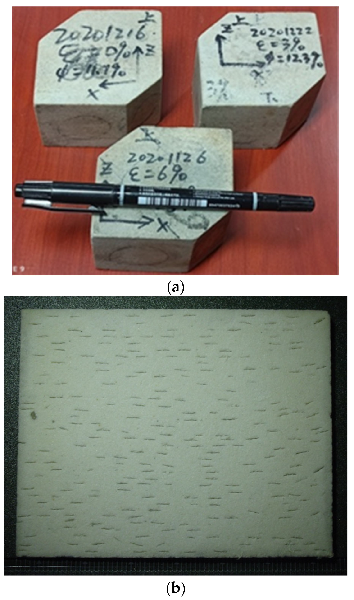
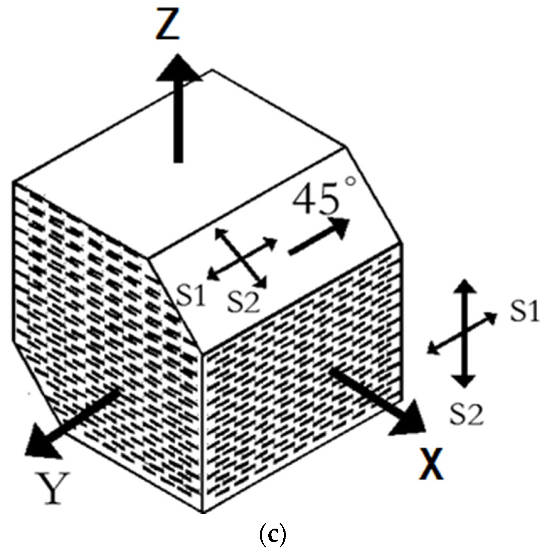
Figure 2.
SEM images of artificial fractured sandstones. (a) Pore structure; and (b) aligned fractures.
Figure 2.
SEM images of artificial fractured sandstones. (a) Pore structure; and (b) aligned fractures.
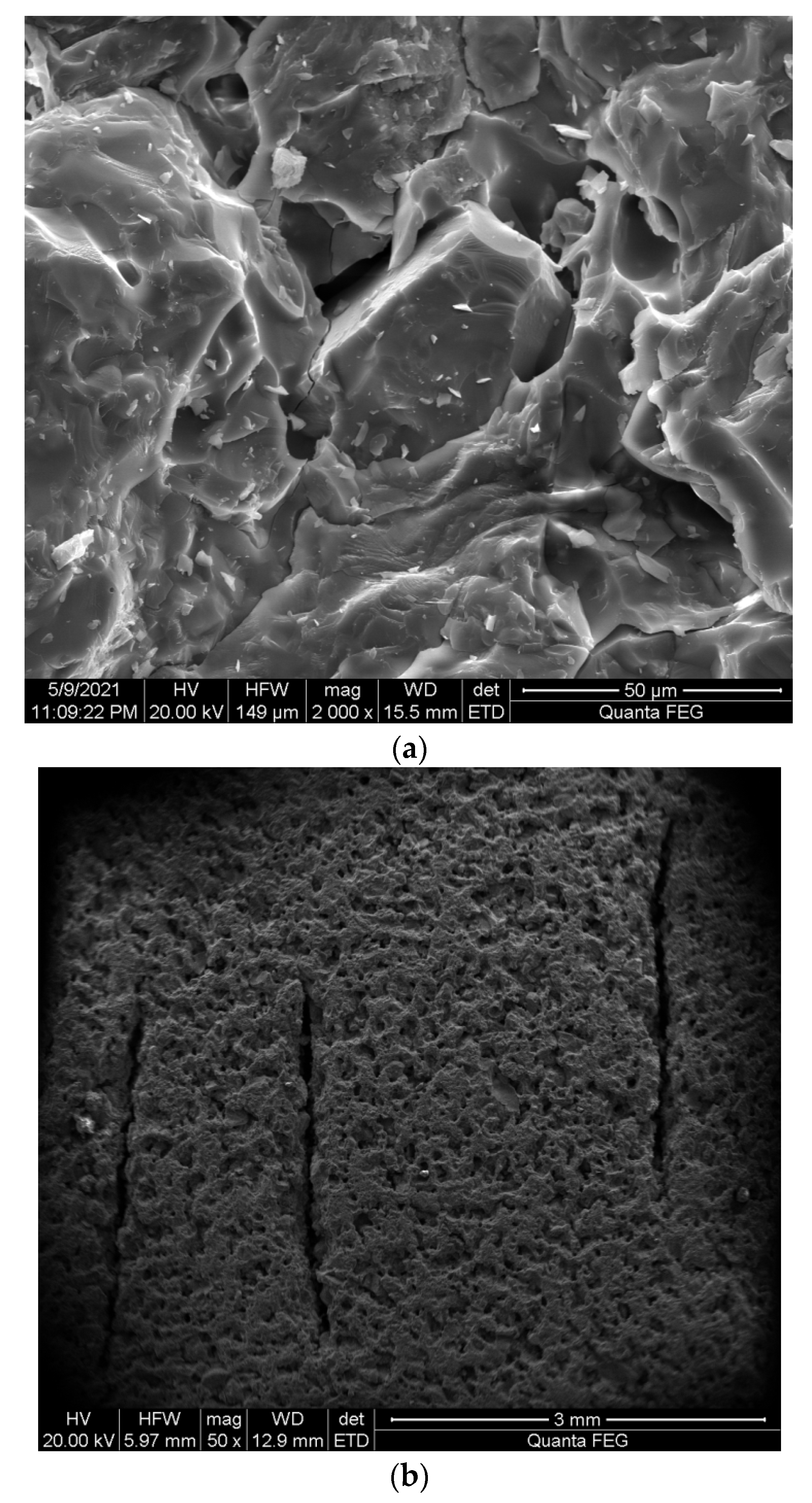
Figure 6.
Measured anisotropy and theoretical predictions of the Galvin model. (a) P-wave anisotropy; (b) S-wave anisotropy.
Figure 6.
Measured anisotropy and theoretical predictions of the Galvin model. (a) P-wave anisotropy; (b) S-wave anisotropy.
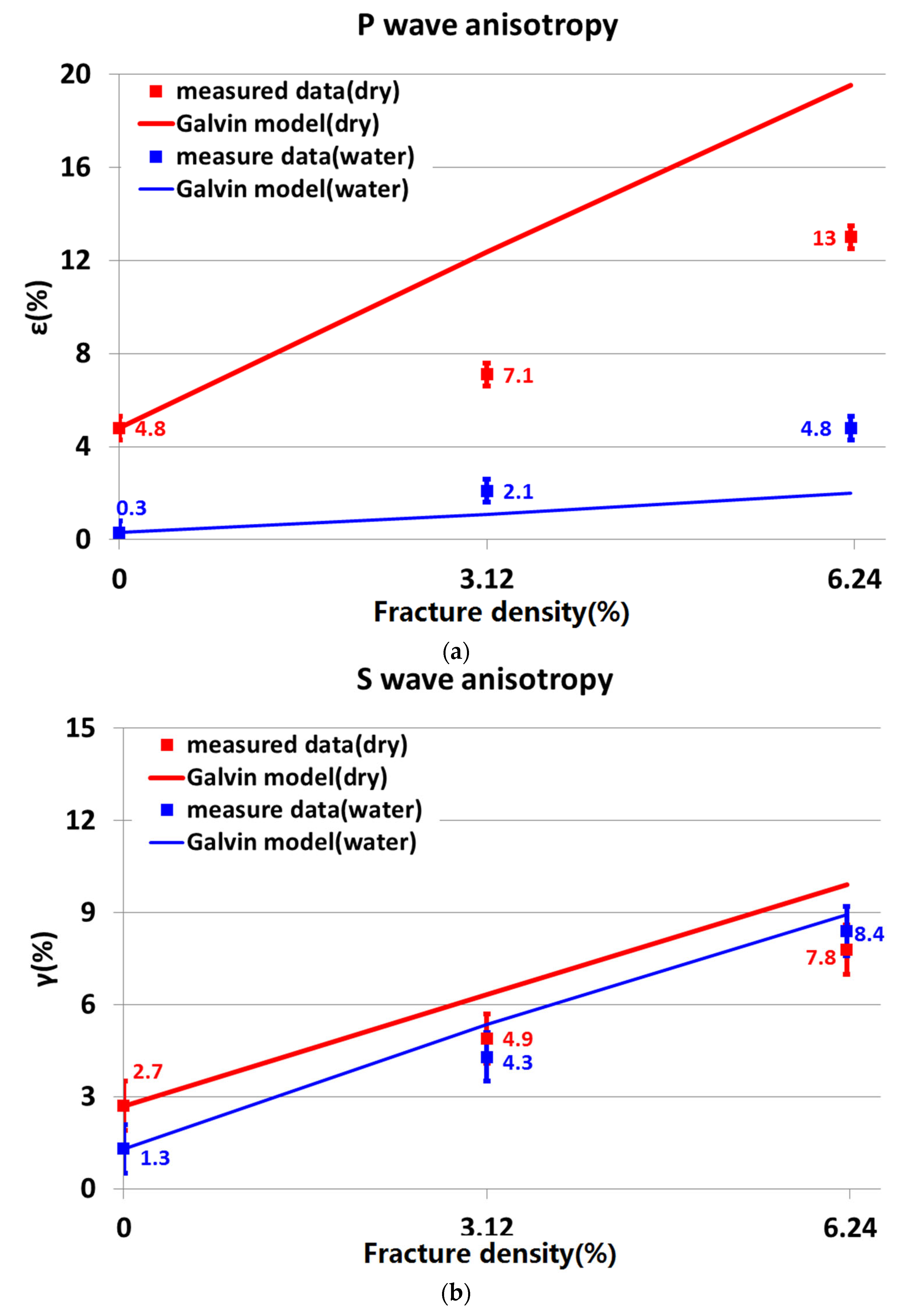
Figure 7.
Measured velocity and theoretical predictions of the Galvin model (dashed curves) and the modified model (solid curves) for sample 1# (fracture density 0). (a) P-wave (P-wave velocity measurement error is smaller than the size of labels); (b) SH-wave; and (c) SV-wave.
Figure 7.
Measured velocity and theoretical predictions of the Galvin model (dashed curves) and the modified model (solid curves) for sample 1# (fracture density 0). (a) P-wave (P-wave velocity measurement error is smaller than the size of labels); (b) SH-wave; and (c) SV-wave.
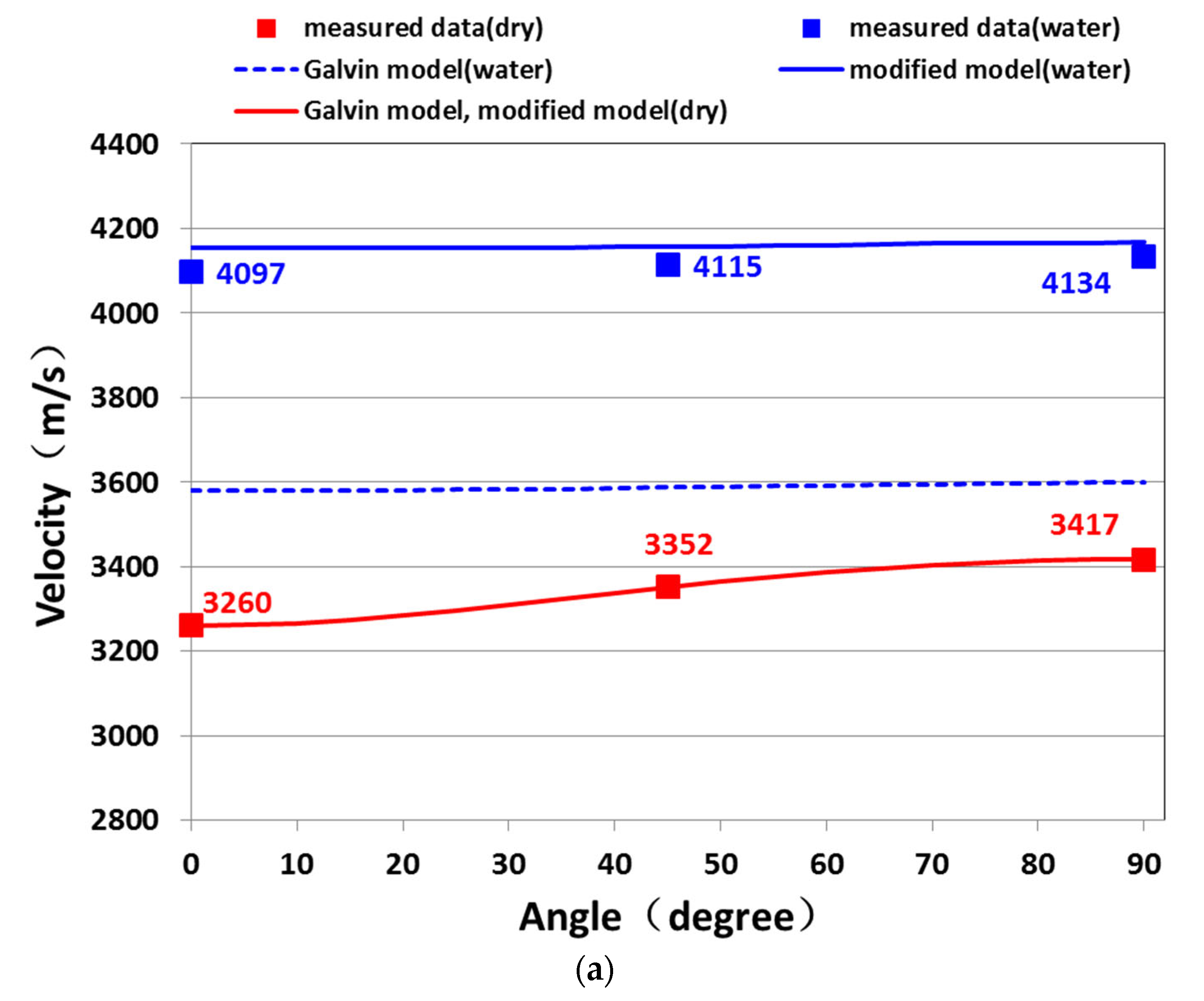
Figure 8.
Measured velocity and theoretical predictions of the Galvin model (dashed curves) and the modified model (solid curves) for sample 2# (fracture density 0.0312). (a) P-wave (P-wave velocity measurement error is smaller than the size of labels); (b)-SH-wave; and (c) SV-wave.
Figure 8.
Measured velocity and theoretical predictions of the Galvin model (dashed curves) and the modified model (solid curves) for sample 2# (fracture density 0.0312). (a) P-wave (P-wave velocity measurement error is smaller than the size of labels); (b)-SH-wave; and (c) SV-wave.
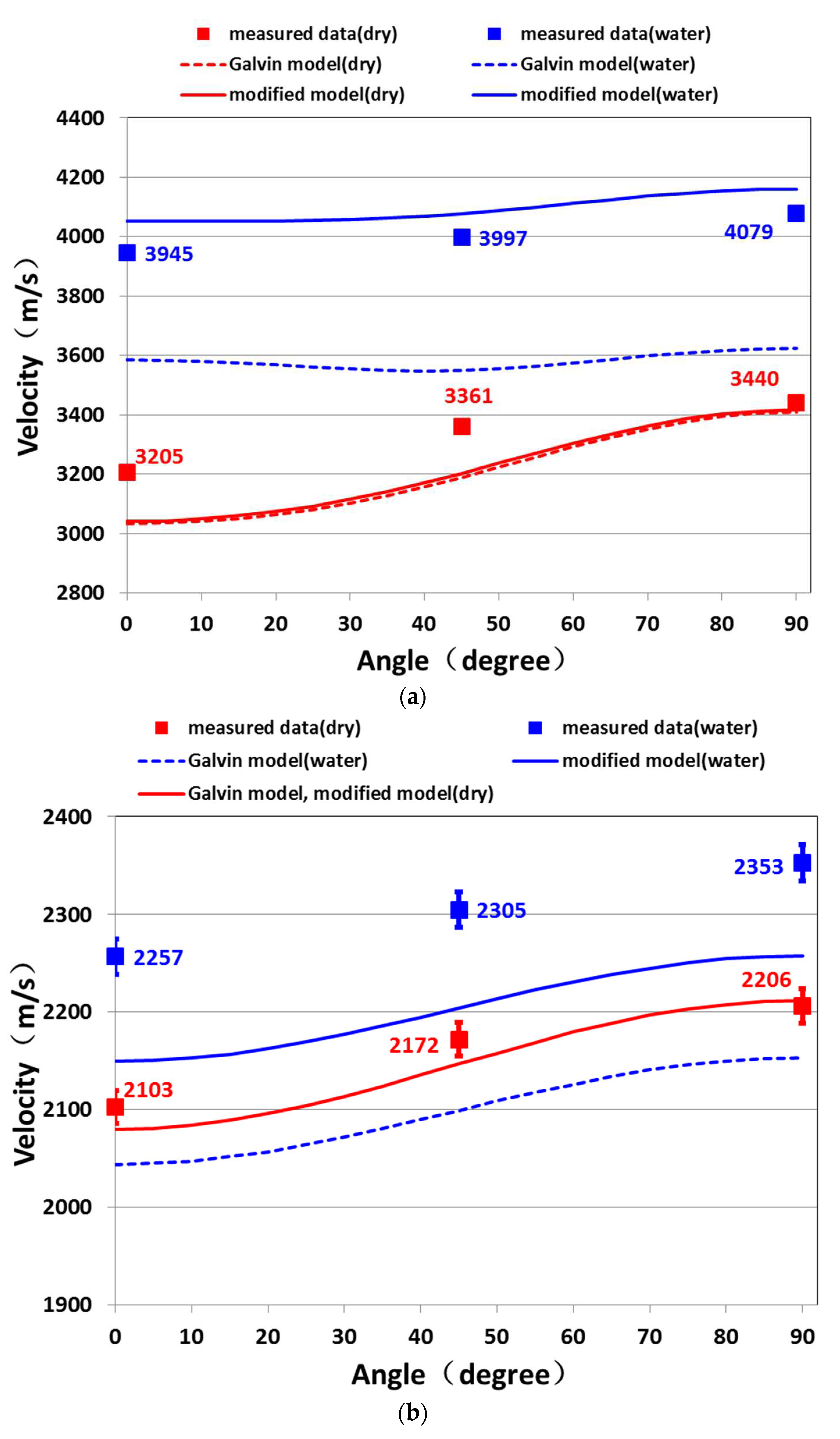
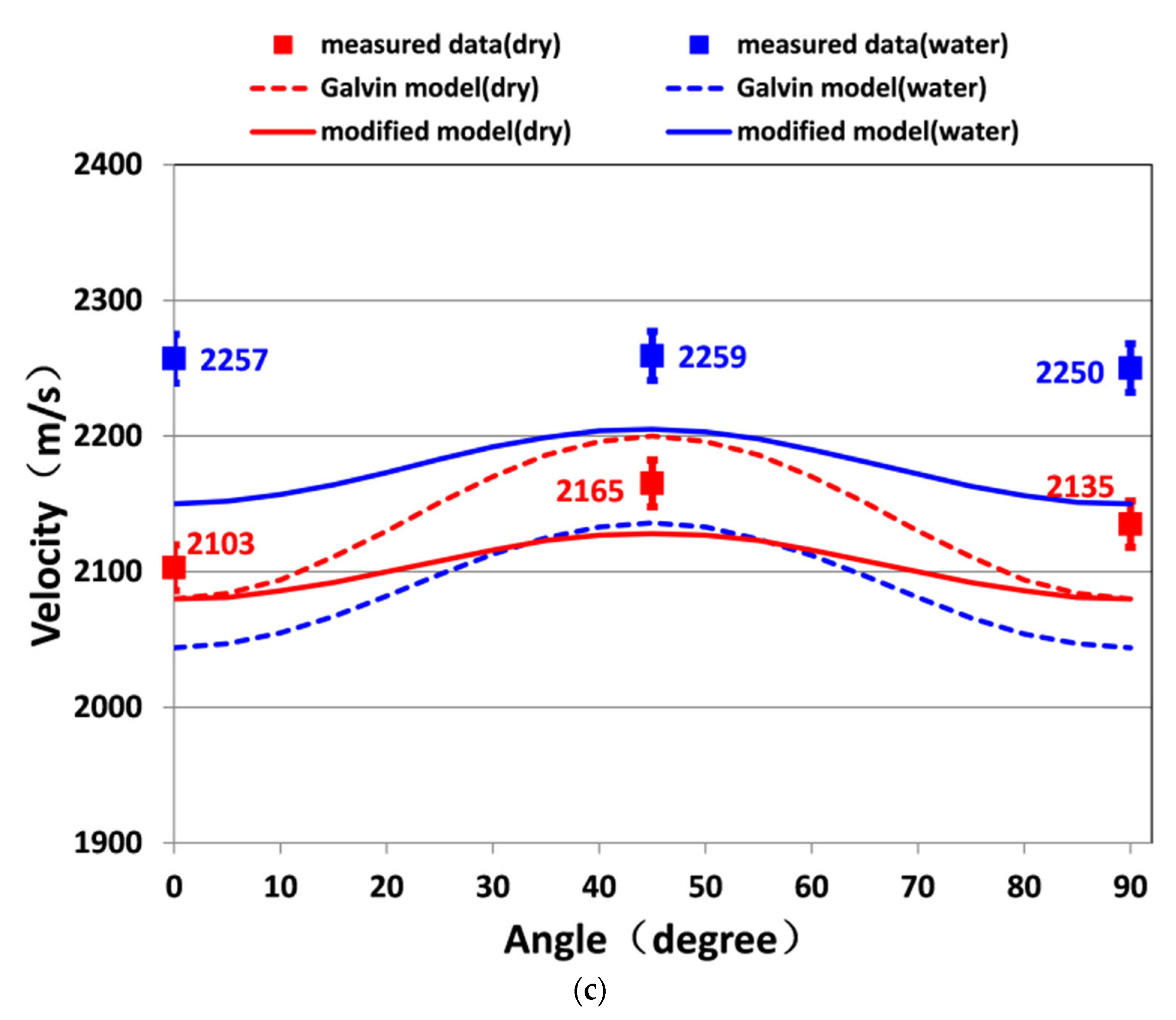
Figure 9.
Measured velocity and theoretical predictions of the Galvin model (dashed curves) and the modified model (solid curves) for sample 3# (fracture density 0.0624). (a) P-wave (P-wave velocity measurement error is smaller than the size of labels); (b) SH-wave; and (c) SV-wave.
Figure 9.
Measured velocity and theoretical predictions of the Galvin model (dashed curves) and the modified model (solid curves) for sample 3# (fracture density 0.0624). (a) P-wave (P-wave velocity measurement error is smaller than the size of labels); (b) SH-wave; and (c) SV-wave.
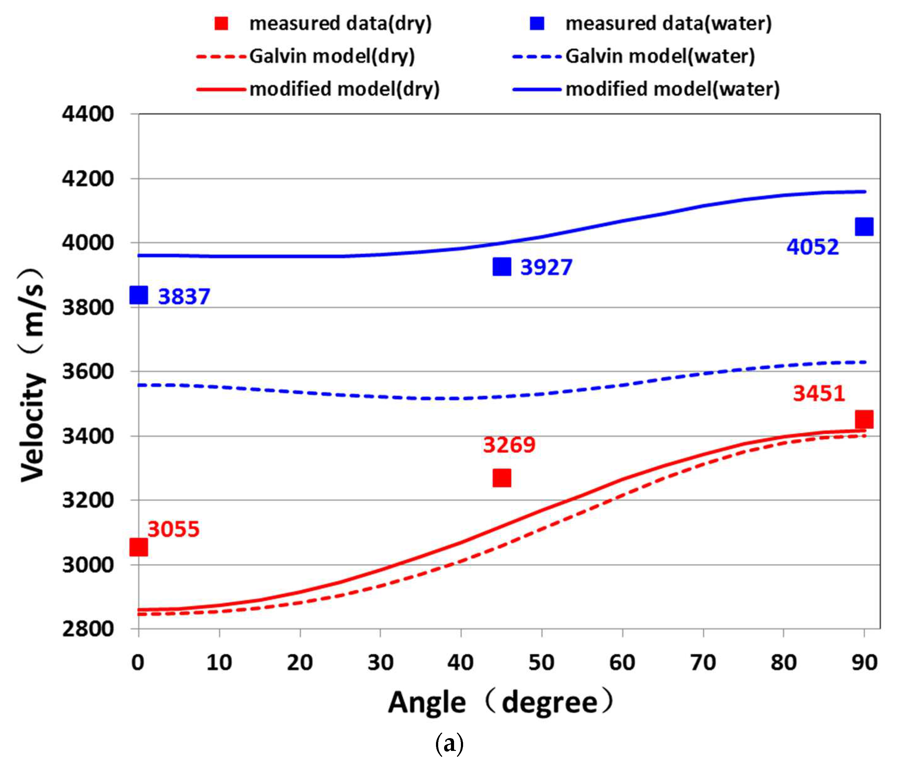
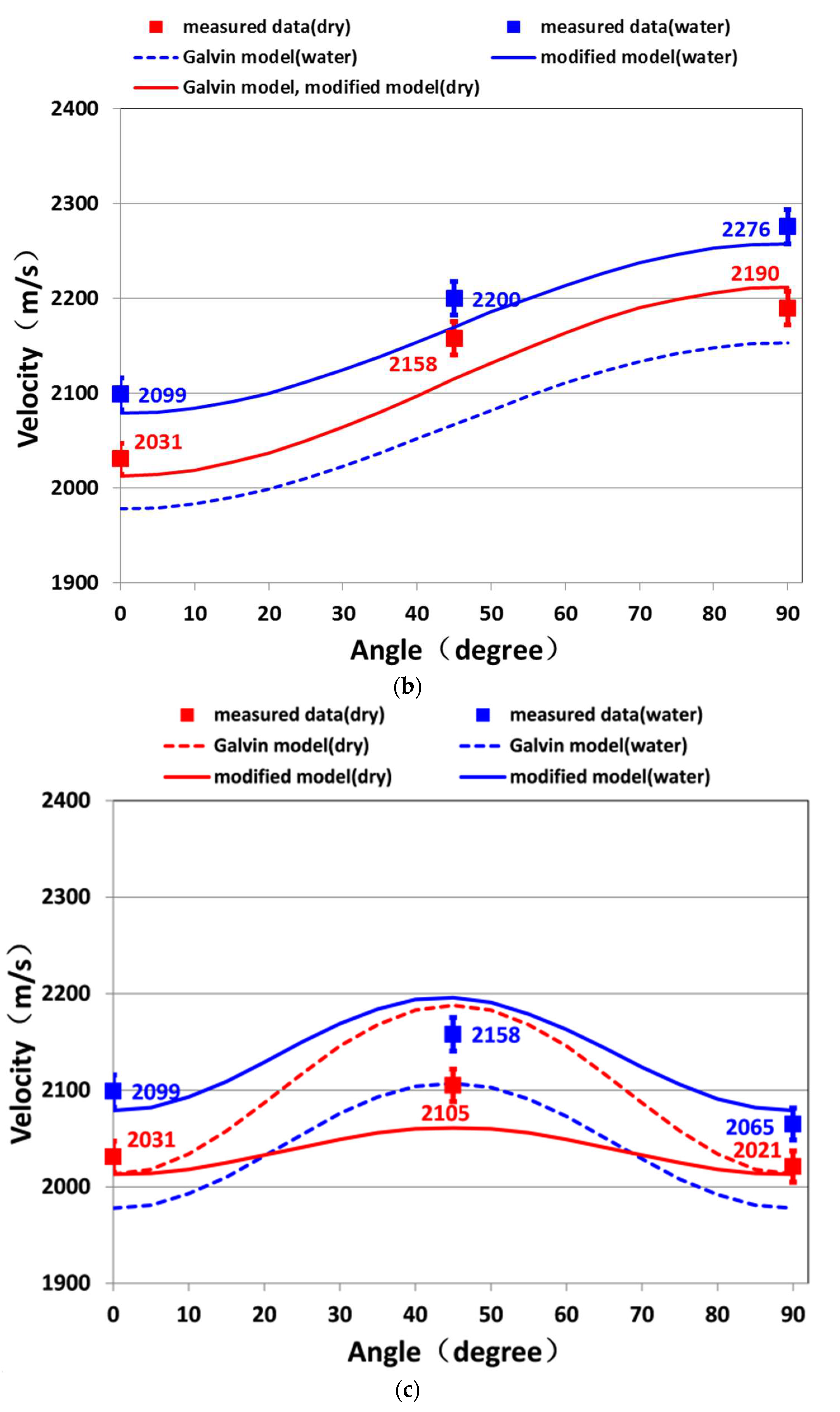
Figure 10.
Measured anisotropy and theoretical predictions of the Galvin model (dashed curves) and the modified model (solid curves). (a) P-wave anisotropy; and (b) S-wave anisotropy.
Figure 10.
Measured anisotropy and theoretical predictions of the Galvin model (dashed curves) and the modified model (solid curves). (a) P-wave anisotropy; and (b) S-wave anisotropy.
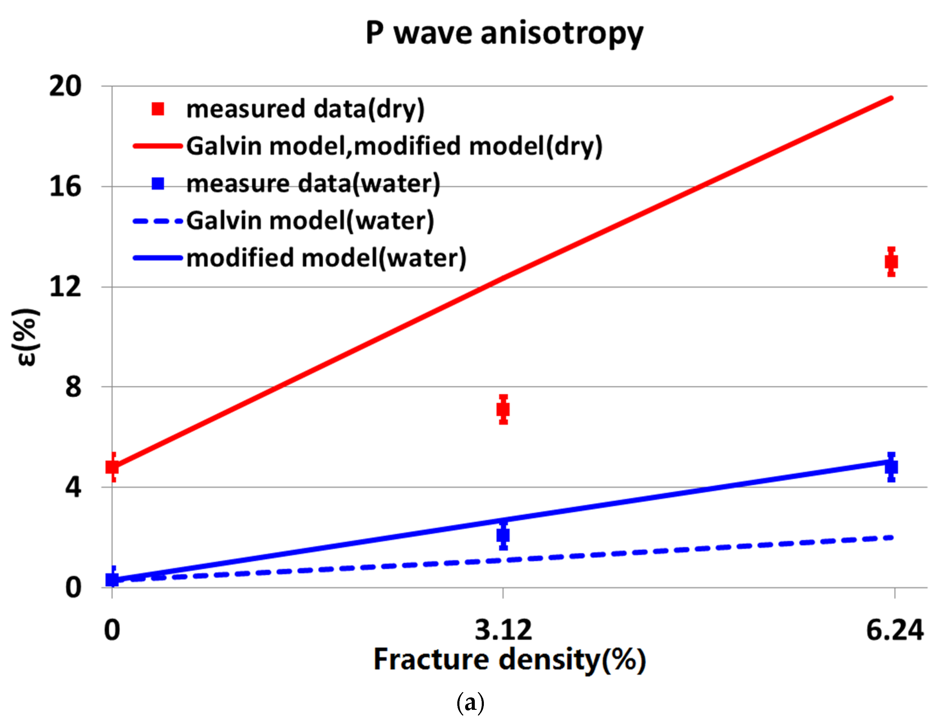
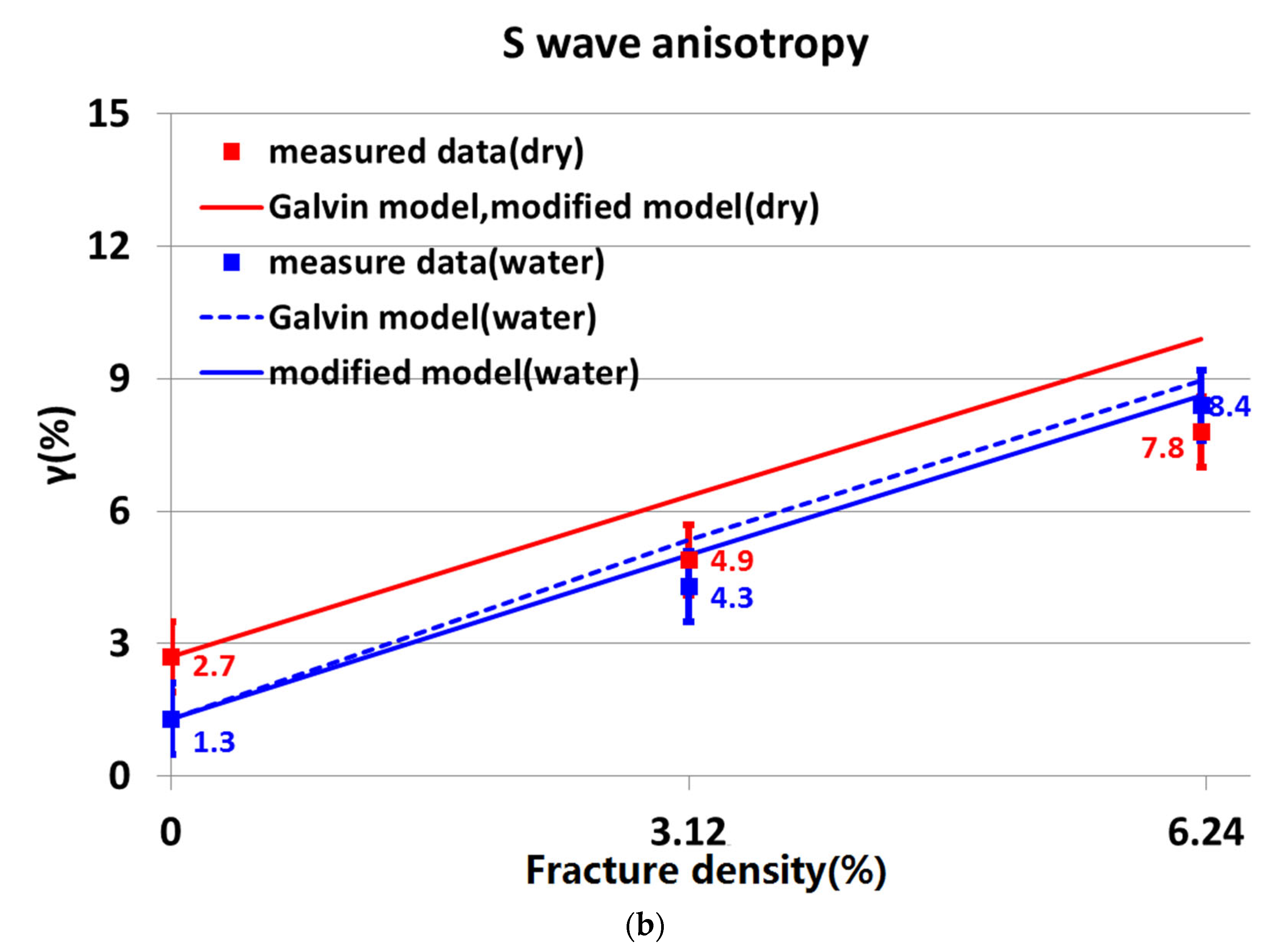

Table 1.
The physical parameters of the three samples.
| Parameters | 1# | 2# | 3# |
|---|---|---|---|
| Number of fracture layers | 49 | 49 | 49 |
| Number of fractures/layers | 0 | 45 | 90 |
| Fracture density | 0 | 0.0312 | 0.0624 |
| Fracture thickness | / | 0.055 mm | 0.055 mm |
| fracture diameter | / | 3 mm | 3 mm |
| Bulk density (air saturation) | 2.114 g/cc | 2.120 g/cc | 2.085 g/cc |
| Bulk density (water saturation) | 2.231 g/cc | 2.243 g/cc | 2.221 g/cc |
| Total porosity | 11.7% | 12.3% | 13.6% |
| Fracture occupied porosity | 0% | 0.36% | 0.72% |
| Matrix porosity | 11.7% | 11.94% | 12.88% |
| Permeability (D) | 0.0013 | / | / |
Table 2.
The scale of the three samples.
| Model Number | Fracture Density |
Length (mm) | |||
|---|---|---|---|---|---|
| X | Y | Z | 45° | ||
| 1# | 0 | 68.54 | 48.75 | 68.46 | 67.03 |
| 2# | 0.0312 | 68.75 | 48.44 | 67.71 | 67.55 |
| 3# | 0.0624 | 68.78 | 49.42 | 68.44 | 67.99 |
Table 3.
Calculated P-wave anisotropy parameter ε in high-, low-, and measured-frequency limits in sample 2#.
Table 3.
Calculated P-wave anisotropy parameter ε in high-, low-, and measured-frequency limits in sample 2#.
| P-wave Anisotropy Parameter ε | |||
|---|---|---|---|
| High Frequency Limit |
Low Frequency Limit |
Measured Frequency (0.5 MHz) | |
| Galvin model | 0.49 | 4.3 | 1.1 |
| Modified model | 2.07 | 4.9 | 2.7 |
Disclaimer/Publisher’s Note: The statements, opinions and data contained in all publications are solely those of the individual author(s) and contributor(s) and not of MDPI and/or the editor(s). MDPI and/or the editor(s) disclaim responsibility for any injury to people or property resulting from any ideas, methods, instructions or products referred to in the content. |
© 2023 by the authors. Licensee MDPI, Basel, Switzerland. This article is an open access article distributed under the terms and conditions of the Creative Commons Attribution (CC BY) license (http://creativecommons.org/licenses/by/4.0/).
Copyright: This open access article is published under a Creative Commons CC BY 4.0 license, which permit the free download, distribution, and reuse, provided that the author and preprint are cited in any reuse.


