Dynamical Analysis of an Age-Structured Sveir Model With Imperfect Vaccine

1. Introduction

Since the proposal of compartmental models and epidemiological theory [1], an increasing number of scholars have utilized these concepts to study the transmission of epidemics. Based on the classic SIR model, it is realistic to incorporate a latent period and vaccination strategy, resulting in an SVEIR model. Recently, these models have been extensively studied [2,3,4,5,6,7,8,9].

Li et al. [2] discussed models of infectious diseases that incorporate incubation and vaccination periods, as well as permanent immunity after recovery. The results in [3] described that assume a negligible probability of infection when the vaccinated person becomes immune or before, the disease can be successfully eliminated and warns against overestimating the effectiveness of vaccination. After simulating the model presented in [4], Upadhyay et al. in modeling computer viruses found that the reinfection rate $\alpha$, is crucial in accurately describing the dynamics of the virus as well as the rate of infection can be reduced by increasing the number of susceptible nodes. Zhang et al. [5] constructed an SVEIR model with two time delays and analyzed the impact of these delay parameters on the dynamical behaviors of the system. In addition, several SVEIR models have been developed to assess the impact of incomplete vaccination on epidemics, such as tuberculosis vaccine [6], hepatitis B vaccine [7], SARS vaccine [8], and HIV vaccine [9].

In recent years, many researchers have taken into account the influence of age on the transmission of epidemics. As a result, a number of age-structured epidemic models have been established, and significant progress has been made. [10,11,12,13,14,15,16,17,18,19,20,21,22,23,24,25].

Röst [10] constructed an SEIR model with age-affected infected individuals, discussed the stability of equilibria, and demonstrated that $k\left(a\right)$ has a direct impact on the value of $R_0$. Griffiths et al. [11] discussed that HIV is most prevalent among individuals aged 20-29, and that HIV prevention activities are most effective when targeted towards individuals under the age of 35. Magal et al. [12] discovered that if the infectious period coincides with the asymptomatic period for even one day, complete eradication of the disease is not possible, even with quarantine measures in place. The analysis presented in [13]suggests that reducing the ratio of vector density to host density is the most effective method to suppress vector diffusion. Moreover, the smaller the ratio, the less likely it is for backward bifurcation to occur, resulting in a smaller basic reproduction ratio. Ebenman [14] explained that when density dependence is primarily influenced by young populations, stabilisation can be achieved through increased competition between young and old populations. On the other hand, species with greater ecological isolation between different age levels are expected to be more stable. Guo et al.[15] suggested that better control of TB spread can be achieved by reducing the TB spread coefficient $\beta$ and lowering the TB infectiousness coefficient $\beta \rho$ in individuals undergoing treatment. Xu et al. [16,17,18] discovered that the conversion rate in the model is age-dependent and increases with age, and the probability of patients transitioning from the incubation period to the infection period also increases. Kenne et al. [19] demonstrated that birth rates can directly impact the stability of diseases and that changing certain parameters can trigger periodic epidemics, making it difficult to eradicate infectious diseases from the population. Li and Wang [20] proposed that to effectively control infectious diseases, it is crucial to maintain a low recruitment rate of susceptible people remains low, and in addition to vaccination, limiting travel and avoiding large gatherings of people are also necessary measures. Wang et al. [21] found that age is an important factor in the spread of AIDS, and that age directly influences the timing and pace of disease outbreaks. In addition to the work mentioned above, more age-structured models have been discussed and can be found in [22,23,24,25].

The rest of the paper is organized as below. Sect. 2 presents an age-structured model, illustrates the existence and uniqueness of equilibrium points, and defines the basic reproduction number of the model. Sect. 3 obtains the asymptotic smoothness and uniform persistence of the semi-flow, and demonstrate the existence of a global attractor. Sect. 4 analyzes the global stability of equilibrium states. In Sect. 5, concludes this work and discusses the results.

2. Mathematical Model and the Existence of Equilibrium Points

In this part, we establish an epidemic model in which the latent period depends on age. In addition, we demonstrate the existence of equilibrium states and calculate the basic reproduction number of the model.

2.1. Mathematical Model

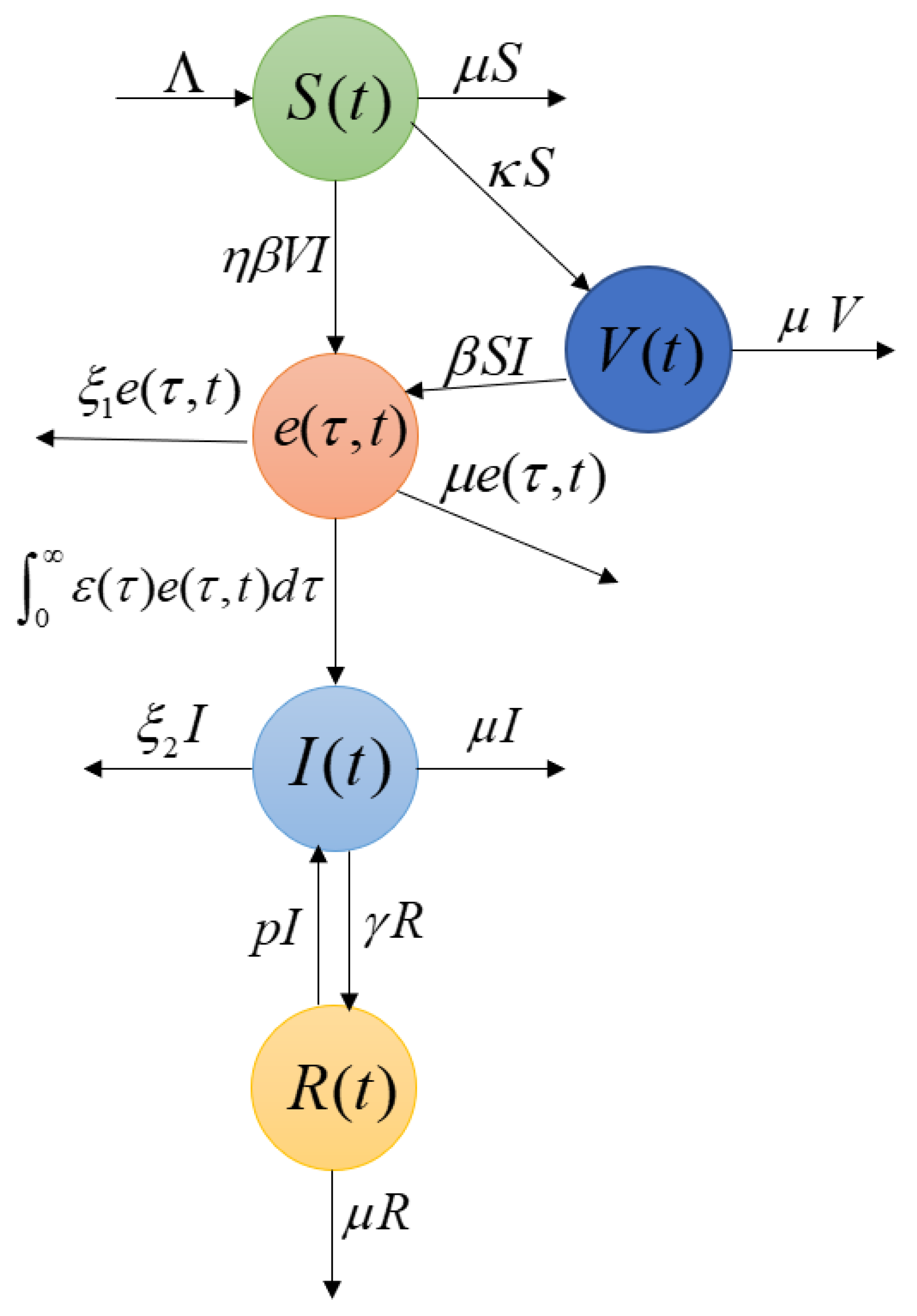
The population is subdivided into five subsets: susceptible, vaccinated, latent, infected, and recovered. Let $S\left(t\right)$, $V\left(t\right)$, $I\left(t\right)$, and $R(t$) be the densities of susceptible individuals, vaccinated individuals, infected individuals, and recovered individuals at time t, respectively. $e(\tau ,t)$ denotes the density of latent individuals aged $\tau$ at time t. Supposing that if a recovered person comes into contact with an infected person, there is a possibility that he or she will relapse into an infected person and continue to participate in the transmission process. Even to a lesser degree, vaccinated individuals are assumed to be susceptible. Suppose that $\Lambda$ is the recruitment rate of susceptible individuals. The susceptible individuals are vaccinated with the rate $\kappa$. $\eta \in (0,1)$ means that the effects of vaccination are imperfect. Let $\beta$ be the rate of infection of susceptible individuals by infected individuals. Latent individuals can become infected at an age-dependent rate is $\epsilon \left(\tau \right)$. Let $\gamma$ and p represent the reinfection rate of the recovered class and the recovery rate of the infected class, respectively. The mortality associated with the latency of the epidemic is ${\xi }_1$ and the epidemic-related mortality in the infected individuals is ${\xi }_2$. Let $\mu$ be the natural mortality rate of the populations. The state variable interactions are shown schematically in Figure 1

Under the above flowchart, the dynamics of the state variables are characterized by differential equations:

$$\left\{\begin{array}{c}{S}^{\prime }=\Lambda -\beta SI-(\mu +\kappa )S,\hfill \\ V^{\prime }=\kappa S-\eta \beta VI-\mu V,\hfill \\ e_{\tau }(\tau ,t)+e_t(\tau ,t)=-(\epsilon \left(\tau \right)+{\xi }_1+\mu )e(\tau ,t),\hfill \\ I^{\prime }={\int }_0^{\infty }\epsilon \left(\tau \right)e(\tau ,t)d\tau -({\xi }_2+p+\mu )I+\gamma R,\hfill \\ R^{\prime }=pI-(\gamma +\mu )R,\hfill \end{array}\right.$$

(1)

which is subject to the following boundary:

$$e{|}_{\tau =0}=\beta SI+\eta \beta VI,$$

(2)

and initial conditions:

$$S{|}_{t=0}=S_0,V{|}_{t=0}=V_0,e{|}_{t=0}=e_0\left(\tau \right),I{|}_{t=0}=I_0,R{|}_{t=0}=R_0,\forall \tau \ge 0,$$

(3)

and $S_0,V_0,I_0,R_0\in R_{+}$, $e_0\left(\tau \right)\in L_{+}^1(0,\infty )$.

To facilitate the calculation, we make the following notations:

$$\sigma \left(\tau \right)=\mu +{\xi }_1+\epsilon \left(\tau \right),\pi \left(\tau \right)=e^{-{\int }_0^{\tau }(\mu +{\xi }_1+\epsilon \left(s\right))ds},\theta ={\int }_0^{\infty }\epsilon \left(\tau \right)\pi \left(\tau \right)d\tau ,\forall \tau \ge 0.$$

(4)

2.2. The Existence of Equilibrium Points

Firstly, through simple calculation, we can get the disease-free equilibrium state of the system (1) is $\ddot{G}=(\frac{\Lambda }{\mu +\kappa },\frac{\psi \Lambda }{\mu (\mu +\kappa )},0,0,0)$, we define:

$$\frac{\Lambda }{\mu +\kappa }:=\ddot{S},\frac{\psi \Lambda }{\mu (\mu +\kappa )}:=\ddot{V}.$$

(5)

Furthermore, we assume that $\widehat{G}=(\widehat{S},\widehat{V},\widehat{e}(·),\widehat{I},\widehat{R})$ is the steady state solution of (1), then $\widehat{G}$ satisfies:

$$\left\{\begin{array}{c}0=\Lambda -\mu \widehat{S}-\kappa \widehat{S}-\beta \widehat{S}\widehat{I},\hfill \\ 0=\kappa \widehat{S}-\mu \widehat{V}-\eta \beta \widehat{V}\widehat{I},\hfill \\ {\widehat{e}}_{\tau }\left(\tau \right)=-\sigma \left(\tau \right)\widehat{e}\left(\tau \right),\hfill \\ 0={\int }_0^{\infty }\epsilon \left(\tau \right)\widehat{e}\left(\tau \right)d\tau -(\mu +{\xi }_2+p)\widehat{I}+\gamma \widehat{R},\hfill \\ 0=p\widehat{I}+(\mu +\gamma )\widehat{R},\hfill \\ \widehat{e}{|}_{t=0}=(\beta \widehat{S}+\eta \beta \widehat{V})\widehat{I}.\hfill \end{array}\right.$$

(6)

Based on [26], we can calculate the basic reproduction number $R_{\rho }$ with the following form:

$$R_{\rho }=\frac{\beta \ddot{S}\theta +\eta \beta \ddot{V}\theta }{(\mu +{\xi }_2+p)-p\gamma /(\mu +\gamma )}.$$

(7)

The 3rd equation of (6) is integrated from 0 to $\tau$, we obtain:

$$\widehat{e}\left(\tau \right)=(\beta \widehat{S}+\eta \beta \widehat{V})\widehat{I}{e}^{-{\int }_0^{\tau }\sigma \left(s\right)ds}=(\beta \widehat{S}+\eta \beta \widehat{V})\widehat{I}\pi \left(\tau \right).$$

(8)

Solving the 1st and the 2nd equation of (6), we have:

$$\left\{\begin{array}{c}\widehat{S}=\frac{\Lambda }{\mu +\kappa +\beta \widehat{I}},\hfill \\ \widehat{V}=\frac{\kappa \Lambda }{(\mu +\eta \beta \widehat{I})(\mu +\kappa +\beta \widehat{I})},\hfill \\ \widehat{R}=\frac{p\widehat{I}}{\mu +\gamma }.\hfill \end{array}\right.$$

(9)

By substituting (7)-(8) into (5), we obtain:

$$h_0{\left(\widehat{I}\right)}^2+h_1\widehat{I}+h_2=0,$$

where

$$\left\{\begin{array}{c}{h}_0=\eta {\beta }^2[(\mu +p+{\xi }_2)(\mu +\gamma )-p\gamma ],\hfill \\ h_1=[(\mu +p+{\xi }_2)(\mu +\gamma )-p\gamma ][(\mu +\kappa )\eta \beta +\mu \beta ]-\eta {\beta }^2\Lambda \theta (\mu +\gamma ),\hfill \\ h_2=[(\mu +p+{\xi }_2)(\mu +\gamma )-p\gamma ]\left[\mu (\mu +\gamma )\right]-\beta \Lambda (\mu +\kappa \eta )(\mu +\gamma )\theta .\hfill \end{array}\right.$$

Let:

$$T\left(\widehat{I}\right)=h_0{\left(\widehat{I}\right)}^2+h_1\widehat{I}+h_2.$$

Clearly, $h_0>0$, so we find that $T\left(\widehat{I}\right)\to \infty$ when $\widehat{I}\to \infty$.

$$\begin{array}{cc}\hfill T\left(0\right)& =h_2=[(\mu +p+{\xi }_2)(\mu +\gamma )-p\gamma ]\left[\mu (\mu +\gamma )\right]-\beta \Lambda (\mu +\kappa \eta )(\mu +\gamma )\theta \hfill \\ \hfill & =\beta \Lambda \theta (\mu +\gamma )(\mu +\kappa \eta )\left(\frac{1}{R_{\rho }}-1\right).\hfill \end{array}$$

(10)

Obviously, when $R_{\rho }>1$, $T\left(0\right)<0$, then according to $T\left(\widehat{I}\right)\in (0,\infty )$ is monotonically increasing, we know that $T\left(\widehat{I}\right)=0$ has only one positive root $\widehat{I}$.

3. Preliminary Results

In this section, we present some results about the semi-flow which generated by (1), such as asymptotic smoothness and uniform persistence.

3.1. The Semi-Flow

Solving the third equation of (1) by using characteristic method, we get:

$$e(\tau ,t)=\left\{\begin{array}{c}{e}_0(\tau -t)\frac{\pi \left(\tau \right)}{\pi (\tau -t)},\tau \ge t\ge 0,\hfill \\ \beta S(t-\tau )+\eta \beta V(t-\tau )\left]I\right(t-\tau \left)\pi \right(\tau ),t>\tau \ge 0.\hfill \end{array}\right.$$

(11)

We start with the following assumptions and later define the state space of system (1).

Assumption 1. 

We make the following hypotheses:

(a) $\epsilon \left(\tau \right)\in L_{+}^1(0,\infty )$ and $\overline{\epsilon }=\underset{\tau \in [0,\infty )}{ess.sup}\epsilon \left(\tau \right)<\infty$;

(b) $\epsilon \left(a\right)$ is Lipschitz continuous on $R^{+}$, that is,$\forall m,v\in \epsilon \left(\tau \right)$,$\left|\epsilon \left(m\right)-\epsilon \left(v\right)\right|\le M_{\epsilon }\left|m-v\right|$;

(c) There exists a ${\mu }_0$ belongs to $(0,\mu ]$ such that $\epsilon \left(\tau \right)\ge {\mu }_0$, $\forall \tau \ge 0$ .

Let the state space of (1) be:

$$\Omega =\left\{S\left(t\right),V\left(t\right),e(·,t),I\left(t\right),R\left(t\right)\in \Sigma \left|S\left(t\right)+V\left(t\right)+{\int }_0^{\infty }e(\tau ,t)d\tau +I\left(t\right)+R\left(t\right)\le \frac{\Lambda }{\mu }\right.\right\}.$$

The function space of the system (1) is defined as:

$$\Sigma =R_{+}^2\times L_{+}^1(0,\infty )\times R_{+}^2$$

and the norm is defined as:

$${∥(x_1,x_2,x_3,x_4,x_5)∥}_{\Sigma }=\left|x_1\right|+\left|x_2\right|+{\int }_0^{\infty }\left|x_3\left(\tau \right)\right|d\tau +\left|x_4\right|+\left|x_5\right|$$

(12)

the initial condition as:

$$x_0=(S_0,V_0,e_0(·),I_0,R_0)\in \Sigma .$$

(13)

According to [27], we can prove that (1) has a unique non-negative solution. Thus, the semi-flow generated by (1) is obtained:

$$\Psi \left(t\right)x_0=(S\left(t\right),V\left(t\right),e(·,t),I\left(t\right),R\left(t\right)),fort\ge 0,x_0\in \Sigma$$

and the norm also can be defined similarly to (12).

Proposition 1. 

For system (1), we know that

(a) $\forall t\ge 0$ , for each $x_0\in \Omega$, we have $\Psi \left(t\right)x_0\in \Omega$;

(b) Ω attracts all points in Σ and Ψ is point dissipative.

Proof. 

We note that $\pi \left(0\right)=1$, $\frac{d}{d\tau }\pi \left(\tau \right)=-\sigma \left(\tau \right)\pi \left(\tau \right)$, and by using the variation of constant formula, we can get:

$${∥\Psi \left(t\right)x_0∥}_{\Sigma }\le \frac{\Lambda }{\mu }-exp(-\mu t)·\left(\frac{\Lambda }{\mu }-{∥x_0∥}_{\Sigma }\right),\forall t\ge 0.$$

(14)

It means that $\Psi \left(t\right)x_0\in \Omega$ for any solution of (1) satisfying $x_0\in \Omega$, $\forall t\ge 0$. Besides, based on (14), for any $\underset{t\to \infty }{lim}∥\Psi \left(t\right)x_0∥\le \Lambda /\mu$, for any $x_0\in \Sigma$. As a result, $\Omega \subseteq \Sigma$attracts all points and $\Psi$ is point dissipative. This proposition has been completely proved. □

Using Assumption 1 and Proposition 1, we obtain the proposition as follows.

Proposition 2. 

Exist $M\ge \frac{\Lambda }{\mu }$, if $x_0\in \Sigma$ and ${∥x_0∥}_{\Sigma }\le M$, then for all $t\ge 0$, we get the following results:

(a) $S\left(t\right),V\left(t\right),{\int }_0^{\infty }e(\tau ,t)d\tau ,I\left(t\right),R\left(t\right)\in [0,M]$;

(b) $e(0,t)\le \beta (1+\eta )M^2$.

3.2. Asymptotic Smoothness

So as to establish global properties of the semi-flow, it is essential to reveal the asymptotic smoothness of the semi-flow ${\left\{\Psi \left(t\right)x_0\right\}}_{t\ge 0}$.

Definition 1.  ([28]) For any nonempty closed bounded set $Z\subset X$ for which $\Psi \left(t\right)Z\subset Z$, if there exists a compact set $Z_0\subset Z$ such that $Z_0$ attracts Z, then $\Psi \left(t\right)x_0:R_{+}\times \Sigma \to \Sigma$ is said to be asymptotically smooth.

Lemma 1.  ([28]) If the following cases are met:

(a) There exists a continuous function $u:R_{+}\times R_{+}\to R_{+}$ such that $\underset{t\to \infty }{lim}u(c,t)=0$ and if ${∥x_0∥}_{\Sigma }\le h$, ${∥{\phi }_1\left(t\right)x_0∥}_{\Sigma }\le u(c,t)$;

(b) ${\phi }_2\left(t\right)x_0$is fully continuous, where t is non-negative,

then $\Psi \left(t\right)x_0={\phi }_1\left(t\right)x_0+{\phi }_2\left(t\right)x_0:R_{+}\times \Sigma \to \Sigma$ is asymptotically smooth in Σ.

Here we divide $\Psi \left(t\right)x_0$ into two operators as follows:

$${\phi }_1\left(t\right)x_0=(0,0,f_3(·,t),0,0),{\phi }_2\left(t\right)x_0=(S\left(t\right),V\left(t\right),{\stackrel{⌣}{f}}_3(·,t),I\left(t\right),R\left(t\right)),$$

where $f_3(\tau ,t)$ and ${\stackrel{⌣}{f}}_3(\tau ,t)$ can be obtained by (6). Clearly,$\Psi \left(t\right)x_0={\phi }_1\left(t\right)x_0+{\phi }_2\left(t\right)x_0$, t is non-negative. To prove (a) of Lemma 1, we need to first confirm the following proposition.

Proposition 3. 

Let $u(c,t)=c{e}^{-(\mu +{\mu }_0)t}$, where $c>0$. Then $\underset{t\to \infty }{lim}u(c,t)=0$ and if ${∥x_0∥}_{\Sigma }\le c$, ${∥{\phi }_1\left(t\right)x_0∥}_{\Sigma }\le u(c,t)$.

Proof. 

Obviously, $u(c,t)$ tend to 0, if $t\to \infty$. From (6), we know:

$$y_3(\tau ,t)=\left\{\begin{array}{c}{e}_0(\tau -t)\frac{\pi \left(\tau \right)}{\pi (\tau -t)},\tau \ge t\ge 0,\hfill \\ 0,t>\tau \ge 0.\hfill \end{array}\right.$$

(15)

For $x_0\in \Omega$ and ${∥x_0∥}_{\Sigma }\le c$, we have:

$$\begin{array}{cc}\hfill & {∥{\phi }_1\left(t\right)x_0∥}_X=\left|0\right|+\left|0\right|+{\int }_0^{\infty }\left|y_3(a,t)\right|da+\left|0\right|+\left|0\right|\hfill \\ \hfill & ={\int }_0^{\infty }\left|e_0\left(\tau \right)\frac{\pi (t+\tau )}{\pi \left(\tau \right)}\right|d\tau \hfill \\ \hfill & ={\int }_0^{\infty }\left|e_0\left(\tau \right)exp\left(-{\int }_{\tau }^{t+\tau }\sigma \left(s\right)ds\right)\right|d\tau .\hfill \end{array}$$

(16)

Note that $\sigma \left(\tau \right)\ge {\mu }_0+\mu +{\xi }_1$, $\forall \tau \ge 0$ holds true, it is easy to get:

$${∥{\phi }_1\left(t\right)x_0∥}_{\Sigma }\le c{e}^{-(\mu +{\mu }_0)t}.$$

(17)

This proposition has been completely proved. □

Since $L_{+}^1(0,\infty )$ is an integral part of $\Sigma$ , we need a compactness concept in $L_{+}^1(0,\infty )$. Next, we take the following result for verifying (b) of Lemma 1.

Based on [29] and the conclusion of Proposition 3, the following confirms that ${\stackrel{⌣}{y}}_3(\tau ,t)$ remains in a precompact subset of $L_{+}^1(0,\infty )$, which is independent of $x_0\in \Omega$. From (11) we have:

$$0\le {\stackrel{⌣}{f}}_3(\tau ,t)=\left\{\begin{array}{c}0,\tau \ge t\ge 0,\hfill \\ \beta S(t-\tau )+\eta \beta V(t-\tau )\left]I\right(t-\tau \left)\pi \right(\tau ),t>\tau \ge 0.\hfill \end{array}\right.$$

(18)

As $\pi \left(\tau \right)=e^{-{\int }_0^{\tau }\sigma \left(s\right)ds}\le e^{-({\mu }_0+\mu +{\xi }_1)\tau }$, then according to (a) of Proposition 2, we derive that ${\stackrel{⌣}{f}}_3(\tau ,t)\le \beta (1+\eta )M^2{e}^{-({\mu }_0+\mu +{\xi }_1)\tau }$. This implies that the condition for a bounded closed set presented in [29] is met. Exist an enough small $c\in (0,t)$, we get:

$$\begin{array}{cc}\hfill & {\int }_0^{\infty }\left|{\stackrel{⌣}{f}}_3(\tau +c,t)-{\stackrel{⌣}{f}}_3(\tau ,t)\right|da={\int }_0^t\left|e(\tau +c,t)-e(\tau ,t)\right|d\tau \hfill \\ \hfill & \le {\int }_0^{t-c}e(0,t-\tau -c)\left|\pi (\tau +c)-\pi \left(\tau \right)\right|d\tau \hfill \\ \hfill & +{\int }_{t-c}^t\left|e(0,t-\tau )\pi \left(\tau \right)\right|d\tau \hfill \\ \hfill & +{\int }_0^{t-c}\left|e(0,t-\tau -c)-e(0,t-\tau )\right|\pi \left(\tau \right)d\tau .\hfill \end{array}$$

We define:

$${\int }_0^{t-c}\left|e(0,t-\tau -c)-e(0,t-\tau )\right|\pi \left(\tau \right)d\tau :=\Delta .$$

Note that $0\le \pi \left(\tau \right)\le e^{-({\mu }_0+\mu +{\xi }_1)\tau }\le 1$, we get:

$$\begin{array}{cc}\hfill & {\int }_0^{t-c}\left|\pi (\tau +c)-\pi \left(\tau \right)\right|d\tau ={\int }_0^{t-c}\pi \left(\tau \right)d\tau -{\int }_c^t\pi \left(\tau \right)d\tau \hfill \\ \hfill & ={\int }_0^{t-c}\pi \left(\tau \right)d\tau -{\int }_c^{t-c}\pi \left(\tau \right)d\tau -{\int }_{t-c}^t\pi \left(\tau \right)d\tau \hfill \\ \hfill & ={\int }_0^c\pi \left(\tau \right)d\tau -{\int }_{t-c}^t\pi \left(\tau \right)d\tau \le c.\hfill \end{array}$$

Hence, from (b) of the Proposition 2, we obtain:

$${\int }_0^{\infty }\left|{\stackrel{⌣}{f}}_3(\tau +c,t)-{\stackrel{⌣}{f}}_3(\tau ,t)\right|d\tau \le 2\beta (1+\eta )M^{2}c+\Delta .$$

Combining (1) and Proposition 2, we have:

$$\left|\frac{dS}{dt}\right|\le \Lambda +(\mu +\kappa )M+\beta M^2,$$

which imply $\left|\frac{dS}{dt}\right|$ is bounded by $K_S=\beta M^2+(\mu +\kappa )M+\Lambda$ and $S\left(t\right)\in [0,\infty )$ is Lipschitz continuous with coefficient $K_S$; $\left|\frac{dV}{dt}\right|$ is bounded by $K_V=-\eta \beta M^2+(\mu +\kappa )M$ and $V\left(t\right)\in [0,\infty )$ is also Lipschitz continuous with Lipschitz coefficient $K_V$. Likewise, from the 4th equation of (1) and Assumption 1, we can also deduce that $\left|\frac{dI}{dt}\right|\le (\mu +{\xi }_2+p)M+\gamma M+\overline{\epsilon }M:=K_I$. It is obviously to get that $I\left(t\right)$ is Lipschitz continuous with coefficient $K_I$. So according to the lemma of Lipschitz continuous [30], we have $SI\in [0,\infty )$ is Lipschitz continuous with coefficient $K_{SI}=(K_S+K_I)M$, $VI\in [0,\infty )$ is also Lipschitz continuous with coefficient $K_{VI}=(K_V+K_I)M$. Hence,

$$\Delta \le {\int }_0^{t-c}\beta (1+\eta )M(K_S+K_V+2K_I)c{e}^{-({\mu }_0+\mu )\tau }d\tau \le \frac{\beta (1+\eta )(K_{SI}+K_{VI})c}{{\mu }_0+\mu }.$$

Based on the above results, we get:

$${\int }_0^{\infty }\left|{\stackrel{⌣}{f}}_3(\tau +c,t)-{\stackrel{⌣}{f}}_3(\tau ,t)\right|d\tau \le \left[2\beta (1+\eta )M^2+\frac{\beta (1+\eta )(K_{SI}+K_{VI})}{{\mu }_0+\mu }\right]c.$$

So $\underset{c\to 0}{lim}{\int }_0^{\infty }\left|{\stackrel{⌣}{f}}_3(\tau +c,t)-{\stackrel{⌣}{f}}_3(\tau ,t)\right|d\tau =0$ is uniformly for any $x_0\in Z$, thus, ${\stackrel{⌣}{f}}_3(\tau ,t)$ remains in a precompact subset $Z_{{\stackrel{⌣}{f}}_3}$ of $L_{+}^1(0,\infty )$. Thus, ${\phi }_2\left(t\right)Z\subset [0,M]\times [0,M]\times Z_{{\stackrel{⌣}{f}}_3}\times [0,M]\times [0,M]$, which is compact in $\Sigma$. Using the lemma of a bounded and closed compact set [30], we can obtain that ${\phi }_2\left(t\right)x_0$ is fully continuous. In summary, Lemma 1 has been completely proved.

In summary, we can get two important theorems as follows.

Theorem 1. 

${\left\{\Psi \left(t\right)x_0\right\}}_{t\ge 0}$ is asymptotically smooth.

Theorem 2. 

${\left\{\Psi \left(t\right)x_0\right\}}_{t\ge 0}$ has a global attractor $\vartheta \in \Sigma$, which attracts the bounded sets of Σ.

3.3. Uniform Persistence

Lemma 2.  ([18]) Consider the following scalar Volterra integro-differential equations:

$$y_t=-hy\left(t\right)+{\int }_0^{\infty }c\left(\alpha \right)y(t-\alpha )d\alpha ,y\left(0\right)>0,$$

where $c(·)\in L_{+}^1(0,\infty )$, $h>0$ and ${\int }_0^{\infty }c\left(\alpha \right)d\alpha >h$. Then the above equation has a unique unbounded solution $y\left(t\right)$.

We denote:

$$\overline{\tau }=inf\left\{\tau :{\int }_{\tau }^{\infty }\epsilon \left(\tau \right)d\tau =0\right\}$$

and define:

$$\stackrel{⌣}{\Sigma }=L_{+}^1(0,\infty )\times R_{+}^2,$$

$$\stackrel{⌣}{B}=\left\{{\left(e\right(·,t),I(t),R(t\left)\right)}^{\prime }\in \stackrel{⌣}{\Sigma }:{\int }_0^{\tau }e(\tau ,t)d\tau >0orI\left(t\right)>0orR\left(t\right)>0\right\}$$

In addition, we make $B=R_{+}^2\times \stackrel{⌣}{B},\partial B=\Sigma \setminus B,\partial \stackrel{⌣}{B}=\stackrel{⌣}{\Sigma }\setminus \stackrel{⌣}{B}$, where B and $\partial B$ are both positively sets. According to [31], we can obtain these results as follows. Before illustrating the uniform persistence of the semi-flow ${\left\{\Psi \left(t\right)x_0\right\}}_{t\ge 0}$, the following theorem is to be proved to hold.

Theorem 3. 

For the semi-flow ${\left\{\Psi \left(t\right)x_0\right\}}_{t\ge 0}$ restricted to $\partial B$, the disease-free equilibrium $\ddot{G}$ of system (1) is globally asymptotically stable.

Proof. 

Let $(S_0,V_0,e_0\left(\tau \right),I_0,R_0)\in \partial B$, so $(e_0\left(\tau \right),I_0,R_0)\in \partial \stackrel{⌣}{B}$. Then we obtain the following system:

$$\left\{\begin{array}{c}{e}_{\tau }(\tau ,t)+e_t(\tau ,t)=-(\mu +{\xi }_1+\epsilon \left(\tau \right))e(\tau ,t),\hfill \\ I^{\prime }={\int }_0^{\infty }\epsilon \left(\tau \right)e(\tau ,t)d\tau -(\mu +{\xi }_2+p)I+\gamma R,\hfill \\ R^{\prime }=pI-(\mu +\gamma )R,\hfill \end{array}\right.$$

(19)

which is subject to the boundary:

$$e{|}_{\tau =0}=(\beta S+\eta \beta V)I,$$

(20)

and initial conditions:

$$e{|}_{t=0}=e_0\left(\tau \right),I{|}_{t=0}=I_0,R{|}_{t=0}=R_0.$$

(21)

As $\underset{t\to \infty }{lim}S\left(t\right)\le \frac{\Lambda }{\mu }$, $\underset{t\to \infty }{lim}V\left(t\right)\le \frac{\Lambda }{\mu }$, from the comparison principle we get:

$$e(\tau ,t)\le \stackrel{⌣}{e}(\tau ,t),I\left(t\right)\le \stackrel{⌣}{I}\left(t\right),R\left(t\right)\le \stackrel{⌣}{R}\left(t\right),$$

(22)

where $(\stackrel{⌣}{e}(\tau ,t),\stackrel{⌣}{I}\left(t\right),\stackrel{⌣}{R}\left(t\right))$ satisfies:

$$\left\{\begin{array}{c}{\stackrel{⌣}{e}}_{\tau }(\tau ,t)+\stackrel{⌣}{e}(\tau ,t)=-(\mu +{\xi }_2+\epsilon \left(\tau \right))\stackrel{⌣}{e}(\tau ,t),\hfill \\ {\stackrel{⌣}{I}}^{\prime }\left(t\right)={\int }_0^{\infty }\epsilon \left(\tau \right)\stackrel{⌣}{e}(\tau ,t)d\tau -(\mu +{\xi }_2+p)I+\gamma R,\hfill \\ {\stackrel{⌣}{R}}^{\prime }\left(t\right)=p\stackrel{⌣}{I}\left(t\right)-(\mu +\gamma )\stackrel{⌣}{R}\left(t\right),\hfill \end{array}\right.$$

(23)

the boundary condition is:

$$\stackrel{⌣}{e}{|}_{\tau =0}=\beta (1+\eta )\frac{\Lambda }{\mu }\stackrel{⌣}{I}\left(t\right),$$

(24)

and initial conditions are:

$$\stackrel{⌣}{e}{|}_{t=0}=e_0\left(\tau \right),I{|}_{t=0}=0,R{|}_{t=0}=0.$$

(25)

Same as (11) and (12), calculating the 1st equation of (25), we get:

$$\stackrel{⌣}{e}(\tau ,t)=\left\{\begin{array}{cc}\hfill & {\stackrel{⌣}{e}}_0(\tau -t)\frac{\pi \left(\tau \right)}{\pi (\tau -t)},\tau \ge t\ge 0,\hfill \\ \hfill & \beta (1+\eta )\frac{\Lambda }{\mu }\stackrel{⌣}{I}(t-\tau )\pi \left(\tau \right),t>\tau \ge 0.\hfill \end{array}\right.$$

(26)

Substituting (26) into the 2nd equation of system (23), we can obtain:

$${\stackrel{⌣}{I}}^{\prime }\left(t\right)=Q\left(t\right)+\beta (1+\eta )\frac{\Lambda }{\mu }{\int }_0^t\epsilon \left(\tau \right)\pi \left(\tau \right)\stackrel{⌣}{I}(t-\tau )d\tau -(\mu +{\xi }_2+p)\stackrel{⌣}{I}\left(t\right)+\gamma \stackrel{⌣}{R}\left(t\right),$$

(27)

where

$$Q\left(t\right)={\int }_t^{\infty }\delta \left(\tau \right)e_0(\tau -t)\frac{\pi \left(\tau \right)}{\pi (\tau -t)}d\tau .$$

Since $(e_0\left(\tau \right),I_0,R_0)\in \partial \stackrel{⌣}{B}$, we have $Q\left(t\right)=0$, for $t\ge 0$. So $\stackrel{⌣}{I}\left(t\right)=0$ is the only solution of the following equation:

$$\left\{\begin{array}{c}{\stackrel{⌣}{I}}^{\prime }\left(t\right)=\beta (1+\eta )\frac{\Lambda }{\mu }{\int }_0^t\epsilon \left(\tau \right)\pi \left(\tau \right)\stackrel{⌣}{I}(t-\tau )d\tau +\gamma R\left(t\right)-(\mu +{\xi }_2+p)\stackrel{⌣}{I}\left(t\right),\hfill \\ {\stackrel{⌣}{R}}^{\prime }\left(t\right)=p\stackrel{⌣}{I}\left(t\right)-(\mu +\gamma )\stackrel{⌣}{R}\left(t\right),\hfill \end{array}\right.$$

(28)

the initial conditions are:

$$\stackrel{⌣}{I}{|}_{t=0}=I_0,\stackrel{⌣}{R}{|}_{t=0}=R_0.$$

(29)

From(26), for $0\le \tau <t$, we have $\stackrel{⌣}{e}(\tau ,t)=0$. When $\tau \ge t$, we have:

$${∥\stackrel{⌣}{e}(\tau ,t)∥}_{L^1}={\int }_t^{+\infty }{e}_0(\tau -t)\frac{\pi \left(\tau \right)}{\pi (\tau -t)}d\tau \le e^{-(\mu +{\mu }_0)t}{∥e_0(\tau -t)∥}_{L_{+}^1}.$$

We know that $\underset{t\to 0}{lim}\stackrel{⌣}{e}(\tau ,t)=0$. Hence, $\underset{t\to \infty }{lim}e(\tau ,t)=0$. Furthermore, by the system (1), we can deduce $\underset{t\to \infty }{lim}S\left(t\right)=\ddot{S}$, $\underset{t\to \infty }{lim}V\left(t\right)=\ddot{V}$. Thus, $\ddot{G}$ is globally asymptotically stable in $\partial B$. This theorem has been completely proved. □

We will then demonstrate the uniform persistence of ${\left\{\Psi \left(t\right)x_0\right\}}_{t\ge 0}$.

Theorem 4. 

If $R_{\rho }>1$, then the semi-flow ${\left\{\Psi \left(t\right)x_0\right\}}_{t\ge 0}$ is uniformly persistent with respect to $(B,\partial B)$. This means that there exists a $\epsilon >0$ such that$\underset{t\to \infty }{lim}{∥\Psi \left(t\right)x_0∥}_{\Sigma }\ge \epsilon$ for any $x_0\in B$. Furthermore, there exist a compact global attractor ${\vartheta }_0\in B$ of ${\left\{\Psi \left(t\right)x_0\right\}}_{t\ge 0}$.

Proof. 

Based on Theorem 3, we only need to demonstrate that there exist $\overline{T}\ge 0$ and $\epsilon >0$ such that $\underset{t\to \infty }{lim}{∥\Psi \left(t\right)x_0∥}_{\Sigma }\ge \epsilon$, $\forall x_0\in B$. This can be shown as follows:

$$W^S\left(\ddot{G}\right)\cap B=⌀,$$

where

$$W^S\left(\ddot{G}\right)=\left\{x_0\in B:\underset{t\to \infty }{lim}\Psi \left(t\right)x_0=\ddot{G}\right\}.$$

On the contrary, we suppose that $\exists f_0\in B$ such that $\underset{t\to \infty }{lim}\Psi \left(t\right)f_0=\ddot{G}$. Then, for t is non-negative, we can discover a sequence $\left\{f_n\right\}\subset B$ such that:

$${∥\Psi \left(t\right)f_n-\ddot{G}∥}_{\Sigma }\le \frac{1}{n}$$

Denote:

$$\Psi \left(t\right)f_n=(S_n\left(t\right),V_n\left(t\right),e_n(·,t),I_n\left(t\right),R_n\left(t\right)),$$

$$f_n=(S_n\left(0\right),V_n\left(0\right),e_n\left(0\right),I_n\left(0\right),R_n\left(0\right)).$$

We can select a sufficiently big $n>0$ such that $\ddot{S}-\frac{1}{n}>0$, $\ddot{V}-\frac{1}{n}>0$. For the selected $n>0$ and there exists a $\overline{T}$ is positive, when $t>\overline{T}$, we have:

$$\begin{array}{cc}\hfill \ddot{S}-\frac{1}{n}<S_n\left(t\right)<& \ddot{S}+\frac{1}{n},\hfill \\ \hfill \ddot{V}-\frac{1}{n}<V_n\left(t\right)<& \ddot{V}+\frac{1}{n},\hfill \\ \hfill -\frac{1}{n}<I_n\left(t\right)<& \frac{1}{n},\hfill \\ \hfill -\frac{1}{n}<R_n\left(t\right)<& \frac{1}{n}.\hfill \end{array}$$

(30)

By the (11) and (12), we obtain:

$$e(\tau ,t)\ge \left[\beta S\right(t-\tau )+\eta \beta V(t-\tau \left)\right]I(t-\tau )\pi \left(\tau \right).$$

(31)

Combining (30)–(31) and the 4th equation of (1), we have:

$$I_n\left(t\right)\ge u_n\left(t\right)$$

where $u_n\left(t\right)$ satisfies:

$$\left\{\begin{array}{c}\frac{d{u}_n\left(t\right)}{dt}={\int }_0^{\infty }\beta \left[\left(\ddot{S}-\frac{1}{n}\right)+\eta \beta \left(\ddot{V}-\frac{1}{n}\right)\right]\epsilon \left(\tau \right)\pi \left(\tau \right)u_n(t-\tau )d\tau \hfill \\ +\gamma u_n\left(t\right)-(\mu +{\xi }_2+p)u_n\left(t\right),\hfill \\ u_n\left(t\right)=I_n{|}_{t=0}\ge 0.\hfill \end{array}\right.$$

When $u_n\left(0\right)=0$, $u_n\left(t\right)>0$. No loss of generality, let $u_n\left(0\right)>0$. By $R_{\rho }>1$, we choose large enough $n\in R_{+}$ to satisfy:

$$\frac{\left[\beta \left(\ddot{S}-\frac{1}{n}\right)+\eta \beta \left(\ddot{V}-\frac{1}{n}\right)\right](\mu +\gamma )\theta }{(\mu +{\xi }_2+p)(\mu +\gamma )-p\gamma }>1.$$

Then we can deduce that:

$${\int }_0^{\tau }\left[\beta \left(\ddot{S}-\frac{1}{n}\right)+\eta \beta \left(\ddot{V}-\frac{1}{n}\right)\right]\epsilon \left(\tau \right)\pi \left(\tau \right)d\tau >(\mu +{\xi }_2+p)-\frac{p\gamma }{\mu +\gamma }.$$

From Lemma 2, we know that $u_n\left(t\right)$ is unbounded. Since $I_n\left(t\right)\ge u_n\left(t\right)$, it is easy to see that $I_n\left(t\right)$ is unbounded. This is in contradiction to the fact that $I_n\left(t\right)$ is bounded. Therefore, the hypothesis is false, $W^S\left(\ddot{G}\right)\cap B=⌀$ holds. According to [20], ${\left\{\Psi \left(t\right)x_0\right\}}_{t\ge 0}$ is uniformly persistent. This theorem has been completely proved. □

4. Stability Analysis of the Equilibrium States

We make use of a Volterra-type function $g\left(x\right)=-1-lnx+x$, and define a function of the following form:

$$\omega \left(\tau \right)={\int }_0^{\infty }\epsilon \left(s\right)e^{-{\int }_{\tau }^s\sigma \left(\tau \right)d\tau }ds.$$

Note that $\omega \left(\tau \right)>0$ for $\tau \ge 0$ and $\omega \left(0\right)=\theta$.

4.1. Global Stability of the Disease-free Equilibrium State

Theorem 5. 

If $R_{\rho }<1$, $\ddot{G}$ is locally asymptotically stable; conversely, it is unstable.

Proof. 

We first perform the following variable transformation:

$$\begin{array}{cc}\hfill & x_1\left(t\right)=S\left(t\right)-\ddot{S},\hfill \\ \hfill & x_2\left(t\right)=V\left(t\right)-\ddot{V},\hfill \\ \hfill & x_3(\tau ,t)=e(\tau ,t),\hfill \\ \hfill & x_4\left(t\right)=I\left(t\right),\hfill \\ \hfill & x_5\left(t\right)=R\left(t\right).\hfill \end{array}$$

By linearizing (1) at $\ddot{G}$, we obtain:

$$\left\{\begin{array}{c}{x}_1^{\prime }\left(t\right)=-(\mu +\kappa )x_1\left(t\right)-\beta \ddot{S}{x}_4\left(t\right),\hfill \\ x_2^{\prime }\left(t\right)=\kappa x_1\left(t\right)-\mu x_2\left(t\right)-\eta \beta \ddot{V}{x}_4\left(t\right),\hfill \\ {x_3}_{\tau }(\tau ,t)+{x_3}_t(\tau ,t)=-(\mu +{\xi }_1+\epsilon \left(\tau \right))x_3(\tau ,t),\hfill \\ x_4^{\prime }\left(t\right)={\int }_0^{\infty }\epsilon \left(\tau \right)x_3(\tau ,t)da-(\mu +{\xi }_2+p)x_4\left(t\right)+\gamma x_5\left(t\right),\hfill \\ x_5^{\prime }\left(t\right)=p{x}_4\left(t\right)-(\mu +\gamma )x_5\left(t\right),\hfill \\ x_3{|}_{\tau =0}=(\beta \ddot{S}+\eta \beta \ddot{V})x_4\left(t\right).\hfill \end{array}\right.$$

(32)

Set:

$$\begin{array}{cc}\hfill & x_1\left(t\right)={\tilde{x}}_1{e}^{\lambda t},\hfill \\ \hfill & x_2\left(t\right)={\tilde{x}}_2{e}^{\lambda t},\hfill \\ \hfill & x_3\left(t\right)={\tilde{x}}_3\left(\tau \right)e^{\lambda t},\hfill \\ \hfill & x_4\left(t\right)={\tilde{x}}_4{e}^{\lambda t},\hfill \\ \hfill & x_5\left(t\right)={\tilde{x}}_5{e}^{\lambda t},\hfill \end{array}$$

(33)

where ${\tilde{x}}_1$, ${\tilde{x}}_2$, ${\tilde{x}}_3\left(\tau \right)$, ${\tilde{x}}_4$, ${\tilde{x}}_5$ to be confirmed later. Substituting (33) into (32), we have:

$$\lambda {\tilde{x}}_1=-(\mu +\kappa ){\tilde{x}}_1-\beta \ddot{S}{\tilde{x}}_4,$$

(34)

$$\lambda {\tilde{x}}_2=\kappa {\tilde{x}}_1-\mu {\tilde{x}}_2-\eta \beta \ddot{V}{\tilde{x}}_4,$$

(35)

$$\left\{\begin{array}{c}\lambda {\tilde{x}}_3\left(\tau \right)+{\tilde{x}}_{3\tau }\left(\tau \right)=-(\mu +{\xi }_1+\epsilon \left(\tau \right)){\tilde{x}}_3\left(\tau \right),\hfill \\ {\tilde{x}}_3\left(0\right)=(\beta \ddot{S}+\eta \beta \ddot{V}){\tilde{x}}_4,\hfill \end{array}\right.$$

(36)

$$\lambda {\tilde{x}}_4={\int }_0^{\infty }\epsilon \left(\tau \right){\tilde{x}}_3\left(\tau \right)d\tau -(\mu +{\xi }_2+p){\tilde{x}}_4+\gamma {\tilde{x}}_5,$$

(37)

$$\lambda {\tilde{x}}_5=p{\tilde{x}}_4-(\mu +\gamma ){\tilde{x}}_5.$$

(38)

According to the 1st equation of (36), we obtain:

$$\begin{array}{cc}\hfill & {\tilde{x}}_3\left(\tau \right)={\tilde{x}}_3\left(0\right)·exp(-\lambda \tau )·exp(-{\int }_0^{\tau }\sigma \left(s\right)ds)\hfill \\ \hfill & =(\beta \ddot{S}+\eta \beta \ddot{V}){\tilde{x}}_4·exp(-\lambda \tau )·exp(-{\int }_0^{\tau }\sigma \left(s\right)ds).\hfill \end{array}$$

(39)

Then we substitute (39) into (37) yields, after calculating we have:

$${\int }_0^{\infty }\epsilon \left(\tau \right)\frac{\mu \beta \Lambda +\eta \beta \kappa \Lambda }{\mu (\mu +\kappa )}·e^{-\lambda \tau }·e^{-{\int }_0^{\tau }\sigma \left(s\right)ds}d\tau -(\mu +{\xi }_2+p)+\frac{\gamma p}{\mu +\gamma +\lambda }-\lambda =0.$$

Then we get the characteristic equation as follow:

$$T\left(\lambda \right)={\int }_0^{\infty }\epsilon \left(\tau \right)\frac{\mu \beta \Lambda +\eta \beta \kappa \Lambda }{\mu (\mu +\kappa )}·e^{-\lambda \tau }·e^{-{\int }_0^{\tau }\sigma \left(s\right)ds}d\tau -(\mu +{\xi }_2+p)+\frac{\gamma p}{\mu +\gamma +\lambda }-\lambda .$$

Apparently, $T\left(\lambda \right)$ is continuous and meets:

$$\left\{\begin{array}{c}T\left(\lambda \right)\to -\infty ,as\lambda \to +\infty ;\hfill \\ T\left(\lambda \right)\to +\infty ,as\lambda \to -\infty ;\hfill \\ T^{\prime }\left(\lambda \right)<0.\hfill \end{array}\right.$$

(40)

Note that:

$$\begin{array}{cc}\hfill & T\left(0\right)=\frac{\mu \beta \Lambda +\eta \beta \psi \Lambda }{\mu (\mu +\psi )}\theta -(\mu +{\xi }_2+p)+\frac{\gamma p}{\mu +\gamma }\hfill \\ \hfill & =(R_{\rho }-1)·\frac{[(\mu +{\xi }_2+p)(\mu +\gamma )-p\gamma ]}{\mu +\gamma }.\hfill \end{array}$$

Obviously, when $R_{\rho }<1$, $T\left(0\right)<0$ and when $R_{\rho }>1$, $T\left(0\right)>0$. Hence, according to (40), we know that if $R_{\rho }<1$, the characteristic equation has a unique real root $\widehat{\lambda }<0$, and $\widehat{\lambda }>0$ if $R_{\rho }>1$. Suppose that $\lambda =x+iy$ is an arbitrary complex solution of characteristic $T\left(\lambda \right)=0$. Then, we know that $0=T\left(\lambda \right)=T(x+iy)\le T\left(x\right)$, that is, $x<\widehat{\lambda }$ since $T\left(\lambda \right)$ is monotonically decreasing. Based on the above analysis, we conclude that $\ddot{G}$ is locally asymptotically stable if $R_{\rho }<1$. Similarly, if $R_{\rho }>1$, $\ddot{G}$ is unstable. This theorem has been completely proved. □

Theorem 6. 

$\ddot{G}$ is globally asymptotically stable when $R_{\rho }<1$.

Proof. 

We consider the Lyapunov function with the following form:

$$L=L_1+L_2+I+L_3,.$$

where

$$\begin{array}{cc}\hfill & L_1=\theta \ddot{S}g\left(\frac{S}{\ddot{S}}\right)+\theta \ddot{V}g\left(\frac{V}{\ddot{V}}\right),\hfill \\ \hfill & L_2={\int }_0^{\infty }\omega \left(\tau \right)e(\tau ,t)d\tau ,\hfill \\ \hfill & L_3=\frac{\gamma }{\mu +\gamma }R.\hfill \end{array}$$

Taking the following equations:

$$\Lambda =(\mu +\kappa )\ddot{S},\kappa \ddot{S}=\mu \ddot{V}.$$

To derive $L_1$, we have:

$$\begin{array}{cc}\hfill & \frac{d{L}_1}{dt}=\theta (\mu +\kappa )\ddot{S}-\theta (\mu +\kappa )S-\theta \beta SI-\frac{\theta {\left(\ddot{S}\right)}^2}{S}(\mu +\kappa )+\theta (\mu +\kappa )\ddot{S}+\theta \beta \ddot{S}I\hfill \\ \hfill & +\theta \kappa S-\theta \mu V-\theta \eta \beta VI+\theta \eta \beta \ddot{V}I-\frac{\theta \ddot{V}\kappa S}{V}+\theta \mu \ddot{V}\hfill \\ \hfill & =\theta \mu \ddot{S}\left(2-\frac{\ddot{S}}{S}-\frac{S}{\ddot{S}}\right)+\theta \kappa \ddot{S}\left(3-\frac{\ddot{S}}{S}-\frac{S\ddot{V}}{\ddot{S}V}-\frac{V}{\ddot{V}}\right)\hfill \\ \hfill & +\theta \beta \ddot{S}I-\theta \beta SI+\theta \eta \beta \ddot{V}I-\theta \eta \beta VI.\hfill \end{array}$$

Note that $\omega \left(0\right)=\theta$ and $e{|}_{\tau =0}=\beta SI+\eta \beta VI$ and according to the integration by parts formula, we have:

$$\begin{array}{cc}\hfill & \frac{d{L}_2}{dt}=-\omega \left(\tau \right){\left.e(\tau ,t)\right|}_{\tau =\infty }+\omega \left(0\right)·e{|}_{\tau =0}+{\int }_0^{\infty }e(\tau ,t)\left[\omega \right(\tau \left)\sigma \right(\tau )-\epsilon (\tau \left)\right]d\tau \hfill \\ \hfill & -{\int }_0^{\infty }\omega \left(\tau \right)\sigma \left(\tau \right)e(\tau ,t)d\tau \hfill \\ \hfill & =-\omega \left(\tau \right){\left.e(\tau ,t)\right|}_{\tau =\infty }+\theta (\beta SI+\eta \beta VI)-{\int }_0^{\infty }\epsilon \left(\tau \right)e(\tau ,t)d\tau .\hfill \end{array}$$

(41)

To derive $L_3$, we have:

$$\frac{d{L}_3}{dt}=\frac{\gamma p}{\mu +\gamma }I-\gamma R.$$

(42)

Combining (40)-(42) and the 4th equation of system (1), we obtain:

$$\begin{array}{cc}\hfill & \frac{dL}{dt}=\theta \mu \ddot{S}\left(2-\frac{\ddot{S}}{S}-\frac{S}{\ddot{S}}\right)+\theta \kappa \ddot{S}\left(3-\frac{\ddot{S}}{S}-\frac{S\ddot{V}}{\ddot{S}V}-\frac{V}{\ddot{V}}\right)\hfill \\ \hfill & +\theta \beta \ddot{S}I+\theta \eta \beta \ddot{V}I+\frac{\gamma p}{\mu +\gamma }I-(\mu +{\xi }_2+p)I\hfill \\ \hfill & =\theta \mu \ddot{S}\left(2-\frac{\ddot{S}}{S}-\frac{S}{\ddot{S}}\right)+\theta \kappa \ddot{S}\left(3-\frac{\ddot{S}}{S}-\frac{S\ddot{V}}{\ddot{S}V}-\frac{V}{\ddot{V}}\right)\hfill \\ \hfill & +(R_{\rho }-1)·I·\frac{[(\mu +{\xi }_2+p)(\mu +\gamma )-p\gamma ]}{\mu +\gamma }.\hfill \end{array}$$

According to algebra–geometry mean formula, we get $\frac{dL}{dt}\le 0$ if $R_{\rho }<1$. Moreover, we can learn that $S=\ddot{S}$, $V=\ddot{V}$, $e(\tau ,t)=0$, $I=0$ and $R=0$ is a sufficient condition for $\frac{dL}{dt}<0$. Therefore, $\ddot{M}=\ddot{G}\subset \Omega$ is the largest subset of $\frac{dL}{dt}=0$, by the LaSalle’s invariance set theorem, we learn that if $R_{\rho }<1$, $\ddot{G}$ is globally asymptotically stable. This theorem has been completely proved. □

4.2. Global Stability of the Endemic Equilibrium State

Theorem 7. 

If $R_{\rho }>1$, $\widehat{G}$ is globally asymptotically stable.

Proof. 

We construct the Lyapunov function as:

$$W=W_1+W_2+W_3+W_4,$$

where

$$\begin{array}{cc}\hfill & W_1=\theta \widehat{S}g\left(\frac{S}{\widehat{S}}\right)+\theta \widehat{V}g\left(\frac{V}{\widehat{V}}\right),\hfill \\ \hfill & W_2={\int }_0^{\infty }\omega \left(\tau \right)\widehat{e}\left(\tau \right)g\left(\frac{e(\tau ,t)}{\widehat{e}\left(\tau \right)}\right)d\tau ,\hfill \\ \hfill & W_3=\widehat{I}g\left(\frac{I}{\widehat{I}}\right),\hfill \\ \hfill & W_4=\frac{\gamma }{\mu +\gamma }\widehat{R}g\left(\frac{R}{\widehat{R}}\right).\hfill \end{array}$$

Note the following equations:

$$\Lambda =\mu \widehat{S}+\kappa \widehat{S}+\beta \widehat{S}\widehat{I},\kappa \widehat{S}=\mu \widehat{V}+\eta \beta \widehat{V}\widehat{I}.$$

By some simple derivations, we have some equations as follows:

$$\begin{array}{cc}\hfill & \frac{d{W}_1}{dt}=\theta \left(1-\frac{\widehat{S}}{S}\right)[\Lambda -\mu S-\kappa S-\beta SI]+\theta \left(1-\frac{\widehat{V}}{V}\right)[\kappa S-\mu V-\eta \beta VI]\hfill \\ \hfill & =\theta \left(1-\frac{\widehat{S}}{S}\right)\left[\mu \widehat{S}\left(1-\frac{S}{\widehat{S}}\right)+\kappa \widehat{S}+\beta \widehat{S}\widehat{I}-\kappa S-\beta SI\right]\hfill \\ \hfill & +\theta \left(1-\frac{\widehat{V}}{V}\right)[\kappa S-\mu V-\eta \beta VI]\hfill \\ \hfill & =\theta \mu \widehat{S}\left(-\frac{\widehat{S}}{S}-\frac{S}{\widehat{S}}+2\right)+\theta \kappa \widehat{S}\left(-\frac{\widehat{S}}{S}-\frac{S\widehat{V}}{\widehat{S}V}-\frac{V}{\widehat{V}}+3\right)\hfill \\ \hfill & +\theta \eta \widehat{V}\widehat{I}\left(\frac{V}{\widehat{V}}-\frac{VI}{\widehat{V}\widehat{I}}-1+\frac{I}{\widehat{I}}\right).\hfill \end{array}$$

(43)

$$\begin{array}{cc}\hfill & \frac{d{W}_2}{dt}=-{\int }_0^{\infty }\omega \left(\tau \right)\widehat{e}\left(\tau \right)\left(1-\frac{\widehat{e}\left(\tau \right)}{e(\tau ,t)}\right)\left(e_{\tau }(\tau ,t)+\sigma \left(\tau \right)e(\tau ,t)\right)\frac{1}{\widehat{e}\left(\tau \right)}d\tau \hfill \\ \hfill & =-{\int }_0^{\infty }\omega \left(\tau \right)\widehat{e}\left(\tau \right)\left(\frac{e(\tau ,t)}{\widehat{e}\left(\tau \right)}-1\right)\left(e_{\tau }(\tau ,t)\frac{1}{e(\tau ,t)}+\sigma \left(\tau \right)\right)d\tau .\hfill \end{array}$$

(44)

Then applying integration by parts, we get:

$$\begin{array}{cc}\hfill & \frac{d{W}_2}{dt}=-{\int }_0^{\infty }\omega \left(\tau \right)\widehat{e}\left(\tau \right)\frac{\partial }{\partial \tau }g\left(\frac{e(\tau ,t)}{e^{*}\left(\tau \right)}\right)d\tau \hfill \\ \hfill & =-\omega \left(\tau \right)\widehat{e}\left(\tau \right){\left.g\left(\frac{e(\tau ,t)}{e^{*}\left(\tau \right)}\right)\right|}_{\tau =\infty }+\theta \widehat{e}\left(0\right)\left(-1-ln\frac{e(0,t)}{\widehat{e}\left(0\right)}+\frac{e(0,t)}{\widehat{e}\left(0\right)}\right)\hfill \\ \hfill & -{\int }_0^{\infty }\delta \left(\tau \right)\widehat{e}\left(\tau \right)\left(-1-ln\frac{e(\tau ,t)}{\widehat{e}\left(\tau \right)}+\frac{e(\tau ,t)}{\widehat{e}\left(\tau \right)}\right)d\tau .\hfill \end{array}$$

(45)

From ${\int }_0^{\infty }\delta \left(\tau \right)\widehat{e}\left(\tau \right)d\tau +\gamma \widehat{R}=(\mu +{\xi }_2+k)\widehat{I}$, the derivative of $W_3$ is:

$$\begin{array}{cc}\hfill & \frac{d{W}_3}{dt}=\left(1-\frac{\widehat{I}}{I}\right)\left[{\int }_0^{\infty }\epsilon \left(\tau \right)e(\tau ,t)d\tau +\gamma R-\frac{I}{\widehat{I}}\left({\int }_0^{\infty }\epsilon \left(\tau \right)\widehat{e}\left(\tau \right)d\tau +\gamma \widehat{R}\right)\right]\hfill \\ \hfill & ={\int }_0^{\infty }\epsilon \left(\tau \right)\widehat{e}\left(\tau \right)\left(\frac{e(\tau ,t)}{\widehat{e}\left(\tau \right)}-\frac{I}{\widehat{I}}-\frac{\widehat{I}e(\tau ,t)}{I\widehat{e}\left(\tau \right)}+1\right)d\tau +\gamma \widehat{R}\left(\frac{R}{\widehat{R}}-\frac{I}{\widehat{I}}\right)\left(1-\frac{\widehat{I}}{I}\right).\hfill \end{array}$$

(46)

By calculation, the derivative of $W_4$ is:

$$\frac{d{W}_4}{dt}=\frac{\gamma }{\mu +\gamma }\left(1-\frac{\widehat{R}}{R}\right)[pI-(\mu +\gamma )R].$$

(47)

Note that:

$${\int }_0^{\infty }\epsilon \left(\tau \right)\widehat{e}\left(\tau \right)d\tau =\theta ·\widehat{e}{|}_{\tau =0}=(\beta \widehat{S}\widehat{I}+\eta \beta \widehat{V}\widehat{I})\theta .$$

Then, combining (43) and (45)-(47), we have:

$$\begin{array}{cc}\hfill & \frac{dW}{dt}=\frac{d{W}_1}{dt}+\frac{d{W}_2}{dt}+\frac{d{W}_3}{dt}+\frac{d{W}_4}{dt}\hfill \\ \hfill & =\theta \mu \widehat{S}\left(-\frac{\widehat{S}}{S}-\frac{S}{\widehat{S}}+2\right)+\theta \kappa \widehat{S}\left(-\frac{\widehat{S}}{S}-\frac{S\widehat{V}}{\widehat{S}V}-\frac{V}{\widehat{V}}+3\right)\hfill \\ \hfill & -\omega \left(\tau \right)\widehat{e}\left(\tau \right){\left.g\left(\frac{e(\tau ,t)}{\widehat{e}\left(\tau \right)}\right)\right|}_{\tau =\infty }+J_1+J_2+J_3\hfill \end{array}$$

(48)

where

$$\begin{array}{cc}\hfill & J_1=\theta \beta \widehat{S}\widehat{I}\left(\frac{I}{\widehat{I}}-\frac{SI}{\widehat{S}\widehat{I}}-\frac{\widehat{S}}{S}+1\right)+\eta \beta \widehat{V}\widehat{I}\left(-1+\frac{V}{\widehat{V}}-\frac{VI}{\widehat{V}\widehat{I}}+\frac{I}{\widehat{I}}\right)\hfill \\ \hfill & -\theta \widehat{e}\left(0\right)·\left(1+ln\frac{e(0,t)}{\widehat{e}\left(0\right)}\right)+\theta ·e{|}_{\tau =0},\hfill \\ \hfill & J_2=-{\int }_0^{\infty }\epsilon \left(\tau \right)\widehat{e}\left(\tau \right)\left[\frac{I}{\widehat{I}}-2+\frac{\widehat{I}e(\tau ,t)}{I\widehat{e}\left(\tau \right)}-ln\frac{e(\tau ,t)}{\widehat{e}\left(\tau \right)}\right]d\tau ,\hfill \\ \hfill & J_3=\gamma \widehat{R}\left(\frac{R}{\widehat{R}}-\frac{I}{\widehat{I}}\right)\left(1-\frac{\widehat{I}}{I}\right)+\frac{\gamma }{\mu +\gamma }\left(1-\frac{\widehat{R}}{R}\right)[pI-(\mu +\gamma )R].\hfill \end{array}$$

In fact, we have the following equation holding:

$$J_2=-{\int }_0^{\infty }\epsilon \left(\tau \right)\widehat{e}\left(\tau \right)g\left(\frac{\widehat{I}e(\tau ,t)}{I\widehat{e}\left(\tau \right)}\right)d\tau -\theta ·\widehat{e}{|}_{\tau =0}·g\left(\frac{I}{I^{*}}\right).$$

(49)

As $(\mu +\gamma )\widehat{R}=p\widehat{I}$, we have:

$$\begin{array}{cc}\hfill & J_3=\gamma \widehat{R}-\frac{\gamma \widehat{R}I}{\widehat{I}}-\frac{\gamma \widehat{I}R}{I}+\gamma \widehat{R}-\frac{\gamma p\widehat{R}I}{(\mu +\gamma )R}+\frac{\gamma pI}{\mu +\gamma }\hfill \\ \hfill & =2\gamma \widehat{R}-\frac{\gamma \widehat{I}R}{I}-\frac{\gamma p\widehat{R}I}{(\mu +\gamma )R}.\hfill \end{array}$$

(50)

Note that $e{|}_{\tau =0}=(\beta S+\eta \beta V)I,\widehat{e}{|}_{\tau =0}=(\beta \widehat{S}+\eta \beta \widehat{V})\widehat{I}$, we have:

$$\begin{array}{cc}\hfill & J_1=\theta \beta \widehat{S}\widehat{I}\left(1-\frac{\widehat{S}}{S}+\frac{I}{\widehat{I}}\right)+\theta \eta \beta \widehat{V}\widehat{I}\left(-1+\frac{I}{\widehat{I}}+\frac{V}{\widehat{V}}\right)-\theta ·\widehat{e}\left(0\right)·\left[1+ln\frac{e(0,t)}{\widehat{e}\left(0\right)}\right]\hfill \\ \hfill & =\theta \widehat{e}\left(0\right)g\left(\frac{I}{\widehat{I}}\right)-\theta \beta \widehat{S}\widehat{I}g\left(\frac{\widehat{S}}{S}\right)+\theta \eta \beta \widehat{V}\widehat{I}g\left(\frac{V}{\widehat{V}}\right)\hfill \\ \hfill & -\theta \beta \widehat{S}\widehat{I}g\left(\frac{\widehat{e}\left(0\right)SI}{e(0,t)\widehat{S}\widehat{I}}\right)-\theta \eta \beta \widehat{V}\widehat{I}g\left(\frac{\widehat{e}\left(0\right)VI}{e(0,t)\widehat{V}\widehat{I}}\right).\hfill \end{array}$$

(51)

Finally, substituting (49)-(51) into (48), we have:

$$\begin{array}{cc}\hfill & \frac{dW}{dt}=\theta \mu \widehat{S}\left(-\frac{\widehat{S}}{S}-\frac{S}{\widehat{S}}+2\right)+\theta \kappa \widehat{S}\left(-\frac{\widehat{S}}{S}-\frac{S\widehat{V}}{\widehat{S}V}-\frac{V}{\widehat{V}}+3\right)\hfill \\ \hfill & -\omega \left(\tau \right)\widehat{e}\left(\tau \right){\left.g\left(\frac{e(\tau ,t)}{\widehat{e}\left(\tau \right)}\right)\right|}_{\tau =\infty }-\theta \beta \widehat{S}\widehat{I}g\left(\frac{\widehat{S}}{S}\right)+\theta \eta \beta \widehat{V}\widehat{I}g\left(\frac{V}{\widehat{V}}\right)\hfill \\ \hfill & -\theta \beta \widehat{S}\widehat{I}g\left(\frac{\widehat{e}\left(0\right)SI}{e(0,t)\widehat{S}\widehat{I}}\right)-\theta \eta \beta \widehat{V}\widehat{I}g\left(\frac{\widehat{e}\left(0\right)VI}{e(0,t)\widehat{V}\widehat{I}}\right)\hfill \\ \hfill & -{\int }_0^{\infty }\epsilon \left(\tau \right)e\left(\tau \right)g\left(\frac{\widehat{I}e(\tau ,t)}{I\widehat{e}\left(\tau \right)}\right)d\tau -\frac{\gamma \widehat{I}R}{I}-\frac{\gamma p\widehat{R}I}{(\mu +\gamma )R}+2\gamma \widehat{R}.\hfill \end{array}$$

(52)

By the equation $\kappa \widehat{S}=\mu \widehat{V}+\eta \beta \widehat{V}\widehat{I}$, we get:

$$\begin{array}{cc}\hfill & \theta \kappa \widehat{S}\left(-\frac{\widehat{S}}{S}-\frac{S\widehat{V}}{\widehat{S}V}-\frac{V}{\widehat{V}}+3\right)+\theta \eta \beta \widehat{V}\widehat{I}g\left(\frac{V}{\widehat{V}}\right)\hfill \\ \hfill & \le -\theta \kappa \widehat{S}\left[g\left(\frac{\widehat{S}}{S}\right)+g\left(\frac{S\widehat{V}}{\widehat{S}V}\right)\right].\hfill \end{array}$$

(53)

Throughout analysis, we know that:

$$-\frac{\gamma \widehat{I}R}{I}-\frac{\gamma p\widehat{R}I}{(\mu +\gamma )R}+2\gamma \widehat{R}\le -\gamma \widehat{R}\left[g\left(\frac{\widehat{I}R}{I\widehat{R}}\right)+\frac{p}{\mu +\gamma }g\left(\frac{I}{R}\right)\right].$$

(54)

In the end, inserting (53) and (54) into (52), we get the derivative of W has:

$$\begin{array}{cc}\hfill & \frac{dW}{dt}\le \theta \mu \widehat{S}\left(-\frac{\widehat{S}}{S}-\frac{S}{\widehat{S}}+2\right)-\theta \kappa \widehat{S}\left[g\left(\frac{\widehat{S}}{S}\right)+g\left(\frac{S\widehat{V}}{\widehat{S}V}\right)\right]\hfill \\ \hfill & -\omega \left(\tau \right)\widehat{e}\left(\tau \right){\left.g\left(\frac{e(\tau ,t)}{\widehat{e}\left(\tau \right)}\right)\right|}_{\tau =\infty }-\theta \beta \widehat{S}\widehat{I}g\left(\frac{\widehat{S}}{S}\right)\hfill \\ \hfill & -\theta \beta \widehat{S}\widehat{I}g\left(\frac{\widehat{e}\left(0\right)SI}{e(0,t)\widehat{S}\widehat{I}}\right)-\theta \eta \beta \widehat{V}\widehat{I}g\left(\frac{\widehat{e}\left(0\right)VI}{e(0,t)\widehat{V}\widehat{I}}\right)\hfill \\ \hfill & -{\int }_0^{\infty }\epsilon \left(\tau \right)\widehat{e}\left(\tau \right)g\left(\frac{\widehat{I}e(\tau ,t)}{I\widehat{e}\left(\tau \right)}\right)d\tau -\gamma \widehat{R}\left[\frac{p}{\mu +\gamma }g\left(\frac{I}{R}\right)+g\left(\frac{\widehat{I}R}{I\widehat{R}}\right)\right]\le 0.\hfill \end{array}$$

Thus, we can obtain that $S=\widehat{S},V=\widehat{V},e(\tau ,t)=\widehat{e}\left(\tau \right),I=\widehat{I},R=\widehat{R}$ is a sufficient condition for $\frac{dW}{dt}<0$. Therefore, $\widehat{M}=\widehat{G}\subset \Omega$ is the largest invariant subset of $\frac{dW}{dt}=0$. According to the LaSalle’s invariance set theorem, we can conclude that if $R_{\rho }>1$, the endemic equilibrium $\widehat{G}$ is globally asymptotically stable. This theorem has been completely proved. □

5. Conclusions

This paper presents an SVEIR model from the perspective of imperfect vaccination and latent age, and investigates the dynamics of disease transmission. We take into account an age structure within a latent class, where the latency is described by a variable associated with age: the latent disease conversion rate $\epsilon \left(\tau \right)$. Utilizing the theorem of the next generation matrix, we obtain the basic reproduction number $R_{\rho }$, which serves as a crucial threshold for controlling the harm caused by a disease. When $R_{\rho }<1$, the disease-free equilibrium $\ddot{G}$ is globally asymptotically stable, which means that the disease will eventually disappear. On the contrary, the endemic equilibrium $\widehat{G}$ is globally asymptotically stable, namely, the disease will become endemic. Besides, it is also necessary to consider the asymptotic smoothness and uniform persistence of the semi-flow generated by the system. This is crucial in proving the existence of global attractors and applying the Lyapunov function method.

To better control the epidemic, we need to reduce $R_{\rho }$. Based on the formula for $R_{\rho }$, we find that $R_{\rho }$ decreases as $\eta$. Therefore, the transmission of an epidemic can be slowed down with less imperfect vaccination. Furthermore, we note that when infected individuals come into contact with susceptible or vaccinated individuals, it can also lead to an increase in $R_{\rho }$. Thus, avoiding contact with infected individuals is also key to controlling the epidemic.

References

- Kermark, W.O.; Mckendrick, A.G. A contribution to the mathematical theory of epidemics. Proceedings of the Royal Society of London. Series A. 1927, 115, 700–721. [Google Scholar]
- Li, J.Y.; Yang, Y.L.; Zhou, Y.C. Global stability of an epidemic model with latent stage and vaccination. Nonlinear Analysis: Real World Applications. 2011, 12, 2163–2173. [Google Scholar] [CrossRef]
- Wang, J.L.; Huang, G.; Takeuchi, Y.; Liu, S. SVEIR epidemiological model with varying infectivity and distributed delays. Mathematical Biosciences and Engineering. 2011, 8, 875–888. [Google Scholar] [CrossRef] [PubMed]
- Upadhyay, R.K.; Kumari, S.; Misra, A.K. Modeling the virus dynamics in computer network with SVEIR model and nonlinear incident rate. Journal of Applied Mathematics and Computing. 2017, 54, 485–509. [Google Scholar] [CrossRef]
- Zhang, Z.; Kundu, S.; Tripathi, J.P.; Bugalia, S. Stability and Hopf bifurcation analysis of an SVEIR epidemic model with vaccination and multiple time delays. Chaos, Solitons and Fractals. 2020, 131, 109483. [Google Scholar] [CrossRef]
- Castillo-Chavez, C.; Song, B. Dynamical models of tuberculosis and their applications. Mathematical Biosciences and Engineering. 2004, 1, 361–404. [Google Scholar] [CrossRef]
- Zou, L.; Ruan, S.G.; Zhang, W.N. An age-structured model for the transmission dynamics of hepatitis B. SIAM Journal on Applied Mathematics. 2010, 70, 3121–3139. [Google Scholar] [CrossRef]
- Gumel, A.B.; McCluskey, C.C.; Watmough, J. An SVEIR Model for Assessing Potential Impact of an Imperfect Anti-Sars Vaccine. Mathematical Biosciences and Engineering. 2006, 3, 485–512. [Google Scholar] [CrossRef] [PubMed]
- Gumel, A.B.; McCluskey, C.C.; van den Driessche, P. Mathematical study of a staged progression HIV model with imperfect vaccine. Bulletin of Mathematical Biology. 2016, 68, 2105–2128. [Google Scholar] [CrossRef] [PubMed]
- Röst, G. SEIR epidemiological model with varying infectivity and infinite delay. Mathematical Biosciences and Engineering. 2008, 5, 389–402. [Google Scholar] [CrossRef]
- Griffiths, J.; Lowrie, D.; Williams, J. An age-structured model for the AIDS epidemic. European Journal of Operational Research. 2000, 124, 1–14. [Google Scholar] [CrossRef]
- Magal, P.; McCluskey, C.C.; Webb, G.F. Lyapunov functional and global asymptotic stability for an infection-age model. Applicable Analysis. 2010, 89, 1109–1140. [Google Scholar] [CrossRef]
- Inaba, H.; Sekine, H. A mathematical model for Chagas disease with infection-age-dependent infectivity. Mathematical Biosciences. 2004, 190, 39–69. [Google Scholar] [CrossRef] [PubMed]
- Ebenman, B. Niche differences between age classes and intraspecific competition in age-structured populations. Journal of theoretical biology. 1987, 124, 25–33. [Google Scholar] [CrossRef]
- Guo, Z.K.; Xiang, H.; Huo, H.F. Analysis of an age-structured tuberculosis model with treatment and relapse. Journal of Mathematical Biology. 2021, 82, 1–37. [Google Scholar] [CrossRef]
- Xu, R. Global dynamics of an epidemiological model with age of infection and disease relapse. Journal of Biological Dynamics. 2018, 12, 118–145. [Google Scholar] [CrossRef] [PubMed]
- Magal, P.; Zhao, X.Q. Global attractors and steady states for uniformly persistent dynamical systems. SIAM journal on mathematical analysis. 2005, 37, 251–275. [Google Scholar] [CrossRef]
- Browne, C.J.; Plyugin, S.S. Global analysis of age-structured within-host virus model. Discrete and Continuous Dynamical Systems Series B. 2013, 18, 1999–2017. [Google Scholar] [CrossRef]
- Kenne, C.; Mophou, G.; Dorville, R.; Zongo, P. A model for brucellosis disease incorporating age of infection and waning immunity. Mathematics. 2022, 10, 670. [Google Scholar] [CrossRef]
- Li, H.; Wang, J. Global dynamics of an SEIR model with the age of infection and vaccination. Mathematics. 2021, 9, 2195. [Google Scholar] [CrossRef]
- Wang, Y.P.; Hu, L.; Nie, L.F. Dynamics of a hybrid HIV/AIDS model with age-structured, self-protection and media coverage. Mathematics. 2023, 11, 82. [Google Scholar] [CrossRef]
- He, Z.R.; Zhou, N. Controllability and stabilization of a nonlinear hierarchical age-structured competing system. Electronic Journal of Differential Equations. 2020, 2020, 1–16. [Google Scholar] [CrossRef]
- Liu, L.L.; Liu, X.N. Global stability of an age-structured SVEIR epidemic model with waning immunity, latency and relapse. International Journal of Biomathematics. 2017, 10, 1750038. [Google Scholar] [CrossRef]
- Huo, H.F.; Yang, P.H.; Xiang, H. Dynamics for an SIRS epidemic model with infection age and relapse on a scale-free network. Journal of the Franklin Institute-Engineering and Applied Mathematics 2019, 356, 7411–7443. [Google Scholar] [CrossRef]
- Khan, A.; Zaman, G. Optimal control strategy of SEIR endemic model with continuous age-structure in the exposed and infectious classes. Optimal Control Applications and Methods. 2018, 39, 1716–1727. [Google Scholar] [CrossRef]
- Diekmann, O.; Heesterbeek, J.A.P.; Metz, J.A. On the definition and the computation of the basic reproduction ratio in models for infectious diseases in heterogeneous populations. Journal of mathematical biology. 1990, 28, 365–382. [Google Scholar] [CrossRef]
- Hale, J.K. Functional Differential Equations. Analytic Theory of Differential Equations: The Proceedings of the Conference at Western Michigan University, Kalamazoo, from 30 April to 2 May 1970. Berlin, Heidelberg: Springer Berlin Heidelberg, 1970, 9-22.
- Hale, J.K.; Waltman, P. Persistence in infinite-dimensional systems. SIAM Journal on Mathematical Analysis. 1989, 20, 388–395. [Google Scholar] [CrossRef]
- Adams, R.A.; Fournier, J.J. Sobolev Space. Academic Press. New York. 2003, pp.38-40.
- McCluskey, C.C. Global stability for an SEI epidemiological model with continuous age-structure in the exposed and infectious classes. Mathematical Biosciences and Engineering. 2005, 9, 819–841. [Google Scholar] [CrossRef]
- Magal, P. Compact attractors for time-periodic age-structured population models. Electronic Journal of Differential Equations. 2001, 2001, 1–35. [Google Scholar]
Figure 1.
Compartment transfer diagram of the model.
Disclaimer/Publisher’s Note: The statements, opinions and data contained in all publications are solely those of the individual author(s) and contributor(s) and not of MDPI and/or the editor(s). MDPI and/or the editor(s) disclaim responsibility for any injury to people or property resulting from any ideas, methods, instructions or products referred to in the content. |
© 2023 by the authors. Licensee MDPI, Basel, Switzerland. This article is an open access article distributed under the terms and conditions of the Creative Commons Attribution (CC BY) license (http://creativecommons.org/licenses/by/4.0/).
Copyright: This open access article is published under a Creative Commons CC BY 4.0 license, which permit the free download, distribution, and reuse, provided that the author and preprint are cited in any reuse.