
Submitted:
01 June 2023
Posted:
02 June 2023
You are already at the latest version
Abstract
Coastal areas situated at lower elevations are becoming more vulnerable to flooding as a result of the accelerating global sea level rise. As the sea level rises, so does the groundwater. Barriers designed to shield against marine flooding do not provide protection against flooding caused by rising groundwater. Despite the increasing threat of groundwater flooding, there is limited knowledge about the relationship between sea level rise and groundwater fluctuations. This hinders the ability to adequately consider sea level rise induced groundwater flooding in adaptation initiatives. This study aims to investigate how local groundwater in Juelsminde, Denmark, responds to changes in sea level and to evaluate the predictability of these changes using a machine learning model. The influence of the sea on the shallow groundwater level has been investigated using six groundwater loggers located between 45 and 210 m from the coast. An initial manual analysis of the data revealed a systematic delay in the rise of water levels from the coast to inland areas, with a delay of approximately 15–17 hours per 50 m of distance. Subsequently, a support vector regression model was used to predict groundwater levels 24 hours into the future. This study shows how the groundwater level in Juelsminde is affected by sea level fluctuations. Results suggest a need for increased emphasis on this topic.
Keywords:
Global sea level rise
; Groundwater fluctuations
; Machine learning model
; Predictability
; Loggers
1. Introduction
The global sea level rise is accelerating due to the melting of ice sheets and the thermal expansion of the oceans as a result of climate change [1,2,3]. This will affect millions of people living in low-lying coastal areas worldwide [1,4,5] and many coastal urban areas are already experiencing the consequences of increased precipitation, more frequent storm events and sea level rise SLR [6].
While SLR poses direct challenges to coastal areas, such as flooding and erosion [7,8,9], groundwater inundation (GWI) is an indirect and increasingly problematic consequence of SLR [8]. Ground water level (GWL), especially in the permeable ground, responds to tidal forces. This narrowing of the unsaturated space between the GWL and infrastructure may lead to GWI. Extremely high tides and SLR will intensify these floods due to a higher groundwater table and reduced unsaturated space to store water from storm events [6,10,11,12,13]. There may be many contributors that can influence GWI. It may consist of a single parameter or multiple parameters coinciding, such as rainfall and high tides during a storm event. Furthermore, low-lying coastal zones are prone to compound flooding, where marine and/or surface flooding can happen simultaneously with GWI [4,9]. Coastal barriers designed to protect against surface water are not effective in preventing flooding from below, making GWI especially problematic. This leaves buildings, basements and both underground and surface infrastructure at risk of flooding [6,8,11,12,14,15]. Consequently, it can lead to contamination of the surface and groundwater with sewage [10].
The role of groundwater is important to fully understand the effect of SLR in coastal areas; however, it is often inadequately addressed in studies related to this topic. The effects of SLR are often assessed using numerical modelling, but there are few studies on modelling and forecasting GWI. This lack of information on GWI in coastal areas means that it is not being adequately considered in planning or adaptation initiatives [6,8,9,12,16]. Modelling GWI requires consideration of all parameters that may influence the GWL during extreme weather events, as well as the risk of compound flooding [9]. So far, many of the models used to investigate these systems have been based on physical principles. However, these models require substantial amounts of information about the system, and even when the data is available, they can be difficult to calibrate. Therefore, machine learning models are gaining popularity among hydrologists because they perform well and require less data input [6].
Existing research papers on the effects of SLR on GWL portray a variety of methods and perspectives, reflecting the complexity of the topic.
Habel et al. 2017 [10] used a groundwater flow model to assess the impact of SLR and high tides on GWI in Waikiki, Honolulu, Hawaii and concluded that an SLR of only approximately 1 m would result in a significant increase in the surface area experiencing GWI and its corresponding ramifications. Bjerkelie et al. 2012 [12] also found that SLR causes groundwater rise (GWR). Using a 3D groundwater flow model, researchers discovered that in New Haven, Connecticut, a 0.91 m SLR scenario resulted in a corresponding 0.91 m increase in the near coast GWL. Furthermore, the model indicated that even a GWL ranging from 5.2–7.3 m above sea level responded to the SLR. Results from Knott et al. 2019 [15] using a groundwater flow model showed that, in coastal New Hampshire, USA, there is an estimated mean rise in GWL of 66% of SLR between 0 and 1 km from the coastline. Additionally, the study found that there is a response in GWL up to 5 km inland (3% of SLR) from the coastline. Similar among these three studies is the conclusion that the models must include more parameters and/or data to enhance their reliability [10,12,15].
In Bowes et al.’s 2019 [6] study, two machine learning models, namely long-short-term memory (LSTM) and recurrent neural networks (RNN), were investigated for their effectiveness in forecasting and modelling GWL in Norfolk, Virginia. A comparison of the models showed that LTSM networks are useful in real-time operational forecasts, and the authors predict that GWL forecasting will become a valuable tool in the future management and modelling of coastal flooding.
Although the described studies have addressed this topic in different localities around the world, no systematic research has been conducted on the impact of SLR on GWL in Denmark.
Therefore, this study aims to investigate how the local groundwater table responds to fluctuations in sea level and to uncover regional variations in the dependence on sea level and precipitation in a small town in Denmark. Finally, the predictability of groundwater fluctuations will be tested using a simple machine-learning model based on the information mentioned above.
2. Materials and Methods
2.1. Study Area and Geological Setting
Juelsminde is located on the eastern coast of Jutland, Denmark, on a peninsula bordered by the Kattegat Sea to the east and Vejle Fjord to the south (Figure 1). Juelsminde is prone to flooding and has been identified as one of the top 10 cities in Denmark that are most at risk of flooding. The nearshore areas are dominated by vacation homes, while the harbour is located in the northern part of the city. Further inland, residential houses dominate. A dike with an elevation of 2.6 m above sea level (masl) protects the buildings located south of the harbour from flooding caused by storm surges. The groundwater level is only 0 to 1 m below the ground surface (mbgs), and large parts of the city are drained through a series of ditches, from which water is pumped over the dike into the Kattegat Sea.
In Figure 1, the near-surface soil types are shown. The Juelsminde area is characterised by glacial sediments in an elevated area to the west, covered by postglacial sediments in a lower lying area to the east. Figure 2 displays a geological cross-section based on well data. The glacial till observed in drilling B2 and towards the west in Figure 1 was deposited during the Pleistocene glaciations when the area was repeatedly covered by ice sheets [17]. The postglacial sediments are dominated by marine sand and, to a lesser extent, organic clay (Gyttja). The marine sand was deposited during the Holocene period, when ice melted and retreated, following the latest glaciation. The sea level rose, causing low-lying areas in Denmark to flood, by the combined effect of sea level rise, and the land still being depressed from the weight of the ice sheets. The land has a much slower response to reaching equilibrium than the ocean. The flooding peaked during the Littorina transgression, which occurred approximately 7,500 years ago. This event is responsible for the lower marine sand layer observed in drilling B2. Marine conditions were established and the gyttja layer found in drilling B2 was deposited. The thickness of the lower marine sand is approximately 1 m, but it may be greater in areas where no organic clay is present and a distinct boundary between the upper and lower marine sand can be distinguished. The organic clay layer has a thickness of 3 m and is composed of silt (Gyttja) containing plant remains and shells.
As the land rose following the ice retreat, the shoreline shifted towards its current position. During this regression, the upper layer of marine sand was deposited. It is up to 10 m thick and described as fine- to medium-grained, well-sorted sand containing shells.
Anthropogenic fillings in the area, typically 1–4 m thick, are expected to be local occurrences related to constructions, and as expected the greatest thickness is found in the harbour area.
2.2. Data
Since 2017, six Rotek loggers have been measuring the GWL every 10 minutes. They are located along to coast-perpendicular profiles, with distances from the coastline between 45 and 210 m (Figure 3).
The northernmost profile is located in an open area devoid of significant buildings, whereas the southern profile extends from the beach just south of the harbour and into the urbanised region behind the dike. In the last quarter of 2021, 14 additional IoT groundwater loggers were installed to investigate the dynamics along the coastline and gain a more comprehensive understanding of spatial variation. The tide gauges were installed along the coastline and in residential areas near the coast, as shown in Figure 3. The Danish Meteorological Institute (DMI) conducts sub-hourly measurements of sea level in Juelsminde harbour. Precipitation amounts in Juelsminde are also recorded by DMI. The data is freely available.
2.3. Data Preparation
The various sources of data require different levels of data processing, as shown in Figure 4. The data obtained from the six Rotek loggers were all corrected for barometric pressure by 100%. Where only a few values were missing, they were calculated using linear interpolation. Major outliers were removed, and staggered sections were aligned with the rest of the data series. The sources of sudden jumps (offsets of sections) in the data are unknown, which means that there is a risk of correcting the wrong section of the data. This uncertainty is one of the reasons why this study focuses on the relative changes in the groundwater table. Therefore, the mean of the data series has been subtracted. The data retrieved from the 14 IoT loggers were corrected based on the terrain, and significant outliers were removed by the company that provided the groundwater loggers. The sea level and precipitation data from the DMI required very little correction. Only a few outliers were removed. All data series that were compared were first standardised to the same resolution before analysis, using either linear interpolation or downscaling.
In this study, two different analyses were carried out. (1) A manual analysis was conducted to examine the groundwater responses to high tide and storm events separately. Based on the results of the manual analysis (2), a machine learning model is constructed to assess the predictability of the groundwater response.
Manual Analysis of Sea Level and Groundwater Interaction
Rises in shallow groundwater levels resulting from large, sudden changes in sea level are typically more distinct and easier to identify and separate from each other than minor variations caused by tidal fluctuations. Additionally, they can be traced further inland, making them ideal for evaluating the systemic response of shallow groundwater to sea level rises. The most significant sea level rises are identified and extracted for analyses.
The analysis was conducted on the six data loggers (Rotek), with the longest available time series, placed in two profiles perpendicular to the coast. The sea level rise is determined by subtracting the mean sea level from the level recorded over the past two days. Through automated peak identification, time periods with a peak prominence over 1.2m and SL above 0.5m are selected and listed in Table 1. Information regarding the scale of the SLR and the time interval covering the period of five days before the peak sea level and the subsequent seven days was gathered. This selection resulted in 30 high tide events with relative amplitudes ranging from 1,22m to 1.96m. An example of automatic selection of high-sea-level events is shown in Figure 5.
The minimum threshold of 1.2 m for relative water level change ensures a high enough signal-to-noise ratio inland while also including a sufficient number of high tide events to evaluate possible correlations. The process of peak selection and subsequent analysis methods were inspired by Bowes et al., 2019 [6]. Modified versions of the available code have been used.
2.4. Response Time from Sea Level Rise
To determine the lag time between the rise of sea level and groundwater, an automated algorithm was used to calculate the time from the peak of sea level rise to the peak of groundwater level rise. Each storm event was analysed by extracting the time interval from both sea level and groundwater level data, with the sea level data being interpolated to match the higher resolution of the groundwater data. The raw data was compared to two filtered datasets using two different methods: (1) a Butterworth low-pass filter and (2) a running mean. These methods were employed to eliminate high frequencies, such as tidal changes, from the data. However, filtering affects the peak amplitude and, therefore, was only used to determine the signal delay. Applying a running mean proved to perform best on this dataset. The delay was found using cross correlation of single loggers with the sea level data. All the results were verified manually.
2.5. Attenuation of Groundwater Peak
The inland amplitude damping of the sea level rise indicates the extent to which a storm surge of a certain size affects the groundwater table. This attenuation was calculated for each event by determining the relative increase in groundwater levels at each logger location. The relative increase in GWL was calculated by subtracting the average GWL measured from 48 to 24 hours prior to the GWL peak from the GWL at peak time.
2.6. Predictive Model
A delayed signal from the SLR and corresponding GWR enables the prediction of the GWL based on the sea level. The approach was to use a quick and simple model to gain insight into its predictive capabilities.
The primary objective of developing a predictive model is to estimate future increases in groundwater levels by considering current and forecasted changes in sea levels. The aim was to construct a model that could provide precise forecasts, and thus, the focus was primarily on calculating changes in groundwater levels one day in advance.
Before developing the model, a specific model type was selected. Based on initial tests using the same input in several simple machine learning models, support vector regression (SVR) provided the most accurate results. An SVR-model is a regression model which determines the best fit based on a defined, acceptable error [18]. The model presented in this article is based on a linear kernel.
The model was partly based on historical and real-time data, with sea level and groundwater observations used as input. Precipitation and sea level forecast data provided by the DMI were used. DMI creates weather and sea level forecasts up to five days in advance. These forecasts can be utilised to generate predictions for groundwater levels, and based on these predictions, a warning system can be developed for areas at risk.
The model was trained on data from each of the six loggers individually, and the results were calculated separately for each logger. Hence, in this study, the model functions as six separate models. The model’s predictive capabilities include 24-hour, 3-day and 5-day forecasts. The input parameters were selected in part based on the initial manual analysis of the data and the response of the groundwater.
In the final model, the input parameters are as follows:
- Groundwater level from the past 4 days
- Sea level from the past 4 days and 1 day into the future (using the DMI 1-day forecast)
- Precipitation from the past 24 hours and 1 day into the future (using the DMI 1-day forecast)
- Sine and cosine curve representing seasonality
The model is trained on 60% of the available data, while the validation and cross-validation data each consist of 20%.
3. Results and Discussion
3.1. Groundwater Wave Characteristics
In a homogeneous medium, we expect to find a linear relationship between distance and time for the propagation of a wave peak. Figure 6 displays a box plot representing the observed delay times at the loggers.
The loggers along the northern area, which are not affected by dikes or buildings, appear to exhibit a linear relationship. The two most coastal positions on the southern profile also appear to reasonably follow the trend, while the farthest logger on the southern profile seems to be influenced by other factors. This can be explained by the natural, high variation in the time lag response of the GWL, as the lag time is expected to be dependent on the magnitude of the sea level rise. The peak response in the GWL is clearly visible in the coastal loggers, but the algorithm had difficulty identifying the resulting rise in the loggers located further away from the coast. This is due to a low signal-to-noise ratio in the logger data, which makes it difficult to identify. Moreover, the further inland the loggers are placed, the greater the possibility that the signal from the SLR is drowned out by responses from precipitation events. Furthermore, the further inland, the more likely that local pumping and drainage may also affects the local groundwater level.
Figure 7 and Figure 8 shows that the amplitude of the groundwater level increases as the distance from the coast increases, while the sea level rise decreases. We expect the amplitude damping in a free aquifer to follow a logarithmic function [19]. With a logarithmic time-axis, the relationship can be estimated by fitting a straight line. However, there are outliers, especially when very large sea level rises occur, resulting in extra high amplitudes. Note that event 14 and 25 have outliers caused by possible mispicks. However, there has not been sufficient arguments to exclude them from the dataset. Figure 9, indicates a semi-linear relationship between the rise in sea level and the corresponding increase in the GWL. This relationship is particularly evident in the most prominent SLR events and in Logger 7, which is closest to the coast. Although, the relationship is also detectable in Logger 3 and Logger 6, it is generally significantly less well defined in the two farthest loggers due to signal reduction.
However, these trends are not entirely straightforward. There is significant variation among different events in terms of both the determination of phase shift and the change in amplitude. This is due to the simplification of the groundwater system in Juelsminde and the expectation of complete reliance on the ocean, particularly as the distance from the coast increases. The farther from the coast, the greater the influence of additional factors.
3.2. Sensitivity and Dependency Analysis
The 14 new loggers did not have time series long enough to contain sufficient events for the previous analysis. However, the data were used to conduct an overview analysis of the groundwater’s dependency and sensitivity to sea level rises and precipitation events (Figure 10). The dependence on sea level fluctuations is determined not only by the storm surge responses but also by the trace of tidal changes in the loggers. In these cases, precipitation has a reinforcing effect on the signal, but it is not the primary cause (blue circles). When the GWL cannot be correlated with sea level changes but mainly responds to precipitation, it belongs in the red (triangle) category. In general, loggers located closer to the coast tend to be more vulnerable to the impacts of sea level changes compared to those situated further inland. However, in certain areas, this principle may not apply to individual loggers, and it is presumed that local conditions may influence which parameters have the greatest impact on the groundwater level in a logger. Therefore, it may be difficult to determine exactly how much different parameters affect the various wells, but it can be generally stated that precipitation affects the GWL in all wells to varying degrees, while the impact of sea level is highly dependent on the distance to the coast. The sea level’s dependence is also an indication of the hydraulic connection between the well location and the ocean. Well no. 20 is located relatively far inland, but it clearly responds to tidal changes. It is located adjacent to a wetland that is connected to the ocean, which explains the rapid response.
3.3. Predictability of Groundwater Fluctuations
Results from the 24-hour predictions are displayed in Figure 11 and Figure 12, with the distance to the coast increasing downward. The time period depicted covers a high-water event and the consequent rise in GWL in six wells. The solid grey line represents the observed change in GWL, while the dotted blue line represents the model’s prediction for 1 day ahead. In addition, precipitation and SL fluctuations are visualised below.
The average correlation coefficient for this high-water event is approximately 90%, which indicates the percentage of variations that can be accounted for by the model. The model also performs well, with a high accuracy rate of 78%, in predicting groundwater levels. The average mean deviation is just below 1cm.
The model, however, has its challenges. Three of the major issues are: (1) an overestimation of the contribution of precipitation; and (2) challenges in predicting the extent of extreme GWL rises and (3) relying heavily on the previous groundwater measurements to calibrate the level in the current well. Overestimating the effect of precipitation on the signal can result in periods of a few hours with significantly higher modelled values than those observed. On the contrary, the inability to model extreme events results in modelled values that are lower than the observed values. Both of these factors result in a significant deviation between the predicted and measured GWL. The reliability on previous measurements results in delayed replications of sudden changes and adjust the level retroactively.
Table 3 provides a brief summary of the model’s overall performance in predicting changes in groundwater levels, specifically for 1, 3 and 5 days ahead.
The indicators adjusted R2 (R2adj) and predicted R2 (R2pred) are used to compare the model performance. R2adj indicates how well terms fit a curve or line, but it adjusts for the number of parameters in a model. This means that if a parameter is included in the model but does not contribute to the model, the R2adj will decrease. If the parameter contributes to the model, R2adj will increase. R2adj will always be less than or equal to R2. R2 is the residual sum of squared errors divided by the total sum of squared errors.
where yi is the dependent variable for observation i.
where n is the sample size and k is the number of variables in the model.
R2pred is also known as PRESS statistics and is used to determine how well a regression model makes predictions. If the data consists of a lot of noise, then R2pred will be low as it is not possible to predict random noise. R2pred is useful to avoid overfitting.
where ŷ(-i) is the predicted value of the response variable for this observation found from the fitted regression equation [20,21].
The numbers show that the modelled values correspond well with the observed values (R2adj), but there are still difficulties with making independent predictions (R2pred). However, the low average is due to a few data anomalies that arise from error correction rather than a rising water table. In addition, the average deviation from the observed values is only a few centimetres. When attempting to predict groundwater changes three days into the future, the R2adj decreases while the ability to make accurate predictions (R2pred) increases. This may be because the model was originally slightly overfitted, resulting in a greater deviation from the observed data but a less constrained fit of the model when calculating the predicted values. On the other hand, it seems unlikely that the model can generate valuable outcomes when trying to forecast groundwater fluctuations five days ahead. Here, both correlation coefficients are negative.
4. Conclusions
Comparing sea level and groundwater data has demonstrated a need for greater emphasis on addressing flooding caused by groundwater following sea levels rise. Especially in countries with extensive coastlines and low-lying coastal infrastructure. Although the impact of a storm surge is most noticeable in the wells located closest to the coast, the response to the strongest storm surges were recorded in a well located 210 m from the coastline, with four rows of houses between its location and the ocean. The response signal experiences a delay that ranges from 16 hours and 45 m near the coast to more than 30 hours 210 m away from the coast. In several cases, it has been difficult to identify the high-water signal in the loggers located far inland, possibly because the signal weakens logarithmically as it moves away from the coast. This means that the impact of factors such as rainfall becomes significant enough to have a comparable amplitude, which can mask the signal from the sea. Meanwhile, the groundwater level closer to the coast is more heavily influenced by the impact of the sea. The greater the magnitude of a sea level rise, the greater the corresponding, but delayed, rise in the groundwater table.
The delayed response allows for the calculation of the predicted response of the shallow groundwater ahead of its onset. The support vector regression model shows promising results when predicting the groundwater response in a logger 24 hours in advance using sea level and rainfall data. However, it would be interesting to introduce further improvements and move from single-step prediction to predicting entire time sequences. Additionally, expanding the model to a multi-output model calculating the groundwater table in all wells simultaneously would eliminate the need for calibrating for each well.
This study highlights the significance of incorporating the influence of sea level on groundwater variations in the development of predictive models and the examination of future groundwater levels. In certain regions, the interaction between the sea and the shallow groundwater table intensifies, underscoring the relevance of including this factor in analyses. Furthermore, when determining appropriate climate adaptation strategies, it is crucial to account for the natural dynamics associated with these phenomena.
Author Contributions
Conceptualization, T.R.A., S.E.P. and A.B.M.; methodology, T.R.A., S.E.P., A.B.M. and R.F.M.; formal analysis, R.F.M., H.H.H. and E.P.H.; investigation, R.F.M., H.H.H. and E.P.H.; data curation, R.F.M., H.H.H. and A.B.M.; writing—original draft preparation, R.F.M., E.P.H. and T.R.A.; writing—review and editing, R.F.M., E.P.H., A.B.M. and T.R.A.; visualization, R.F.M. and T.R.A. All authors have read and agreed to the published version of the manuscript.
Funding
This research was funded by EU LIFE, Grant number LIFE15 IPC/DK/000006/C2C CC, Insero Horsens, Grant number 2020-0044 and Engell Friis Fonden, Grant number 2020-021.
Data Availability Statement
Parts of the data analysed in this study is publicly available and can be found here: https://www.dmi.dk/kontakt/frie-data/. The remaining data required to reproduce the findings of this study are available on request from the corresponding author.
Acknowledgments
The authors would like to thank Hedensted municipality for their assistance and collaboration during the project. The authors also owes thanks to Kirsten Landkildehus Thomsen and Hans Erik Hansen for carrying out field and laboratory work.
Conflicts of Interest
The authors declare no conflict of interest and the funders had no role in the design of the study; collection, analyses or interpretation of data; writing of the manuscript or in the decision to publish the results.
References
- IPPC, IPCC Special Report on the Ocean and Cryosphere in a Changing Climate [H.-O. Pörtner, D.C. Roberts, V. Masson-Delmotte, P. Zhai, M. Tignor, E. Poloczanska, K. Mintenbeck, A. Alegría, M. Nicolai, A. Okem, J. Petzold, B. Rama, N.M. Weyer (Eds.)]; 1st ed.; Cambridge University Press, 2019; ISBN 978-1-00-915796-4.
- Sweet, W.V.; Hamlington, B.D.; Kopp, R.E.; Weaver, C.P.; Barnard, P.L.; Bekaert, D.; Brooks, W.; Craghan, M.; Dusek, G.; Frederikse, T.; et al. Global and Regional Sea Level Rise Scenarios for the United States: Updated Mean Projections and Extreme Water Level Probabilities Along U.S. Coastlines; National Oceanic and Atmospheric Administration, National Ocean Service, Silver Spring, MD, 2022; p. 111;
- Davtalab, R.; Mirchi, A.; Harris, R.J.; Troilo, M.X.; Madani, K. Sea Level Rise Effect on Groundwater Rise and Stormwater Retention Pond Reliability. Water 2020, 12, 1129. [Google Scholar] [CrossRef]
- Sangsefidi, Y.; Bagheri, K.; Davani, H.; Merrifield, M. Data Analysis and Integrated Modeling of Compound Flooding Impacts on Coastal Drainage Infrastructure under a Changing Climate. J. Hydrol. 2023, 616, 128823. [Google Scholar] [CrossRef]
- Robinson, C.E.; Xin, P.; Santos, I.R.; Charette, M.A.; Li, L.; Barry, D.A. Groundwater Dynamics in Subterranean Estuaries of Coastal Unconfined Aquifers: Controls on Submarine Groundwater Discharge and Chemical Inputs to the Ocean. Adv. Water Resour. 2018, 115, 315–331. [Google Scholar] [CrossRef]
- Bowes, B.D.; Sadler, J.M.; Morsy, M.M.; Behl, M.; Goodall, J.L. Forecasting Groundwater Table in a Flood Prone Coastal City with Long Short-Term Memory and Recurrent Neural Networks. Water 2019, 11, 1098. [Google Scholar] [CrossRef]
- Knott, J.F.; Elshaer, M.; Daniel, J.S.; Jacobs, J.M.; Kirshen, P. Assessing the Effects of Rising Groundwater from Sea Level Rise on the Service Life of Pavements in Coastal Road Infrastructure. Transp. Res. Rec. J. Transp. Res. Board 2017, 2639, 1–10. [Google Scholar] [CrossRef]
- Habel, S.; Fletcher, C.H.; Rotzoll, K.; El-Kadi, A.I.; Oki, D.S. Comparison of a Simple Hydrostatic and a Data-Intensive 3D Numerical Modeling Method of Simulating Sea-Level Rise Induced Groundwater Inundation for Honolulu, Hawai’i, USA. Environ. Res. Commun. 2019, 1, 041005. [Google Scholar] [CrossRef]
- Bosserelle, A.L.; Morgan, L.K.; Hughes, M.W. Groundwater Rise and Associated Flooding in Coastal Settlements Due To Sea-Level Rise: A Review of Processes and Methods. Earths Future 2022, 10. [Google Scholar] [CrossRef]
- Habel, S.; Fletcher, C.H.; Rotzoll, K.; El-Kadi, A.I. Development of a Model to Simulate Groundwater Inundation Induced by Sea-Level Rise and High Tides in Honolulu, Hawaii. Water Res. 2017, 114, 122–134. [Google Scholar] [CrossRef] [PubMed]
- Hoover, D.J.; Odigie, K.O.; Swarzenski, P.W.; Barnard, P. Sea-Level Rise and Coastal Groundwater Inundation and Shoaling at Select Sites in California, USA. J. Hydrol. Reg. Stud. 2017, 11, 234–249. [Google Scholar] [CrossRef]
- Bjerklie, D.M.; Mullaney, J.R.; Stone, J.R.; Skinner, B.J.; Ramlow, M.A. Preliminary Investigation of the Effects of Sea-Level Rise on Groundwater Levels in New Haven, Connecticut. 2012. [Google Scholar]
- Trglavcnik, V.; Morrow, D.; Weber, K.P.; Li, L.; Robinson, C.E. Analysis of Tide and Offshore Storm-Induced Water Table Fluctuations for Structural Characterization of a Coastal Island Aquifer. Water Resour. Res. 2018, 54, 2749–2767. [Google Scholar] [CrossRef]
- Habel, S.; Fletcher, C.H.; Anderson, T.R.; Thompson, P.R. Sea-Level Rise Induced Multi-Mechanism Flooding and Contribution to Urban Infrastructure Failure. Sci. Rep. 2020, 10, 3796. [Google Scholar] [CrossRef] [PubMed]
- Knott, J.F.; Jacobs, J.M.; Daniel, J.S.; Kirshen, P. Modeling Groundwater Rise Caused by Sea-Level Rise in Coastal New Hampshire. J. Coast. Res. 2019, 35, 143. [Google Scholar] [CrossRef]
- Cooper, H.M.; Zhang, C.; Selch, D. Incorporating Uncertainty of Groundwater Modeling in Sea-Level Rise Assessment: A Case Study in South Florida. Clim. Change 2015, 129, 281–294. [Google Scholar] [CrossRef]
- Houmark-Nielsen, M. ; Pleistocene stratigraphy and glacial history of the central part of Denmark. Bulletin - Geological Society of Denmark, 1987, 36, 1–189. [Google Scholar] [CrossRef]
- Aurélien Géron. Support Vector Machines. In Hands-On Machine Learning with Scikit-Learn, Keras & TenserFlow - Concepts, Tools, and Techniques to Build Intellegent Systems, 2nd ed. Butterfield, N., Taché, N., Cronni, M., Kelly, B. and Cofer, K.; O’Reilly Media, Inc., Sebastopol, 2019.
- Schwarts, F.W.; Zhang, H. Response of an Unconfined Aquifer to Pumping. In Fundamentals of groundwater. Flahive, R., Powell, D.; John Wiley and sons, New York, 2003, pp. 258-273.
- Dodge, Y. The Consise Encyclopedia of Statistics. Springer, New York, 2008.
- Everitt, B. S.; Skrondal, A. The Cambridge Dictionary of Statistics, 4th ed. Cambridge University Press, Cambridge, 2010.
Figure 1.
Overview map showing the Juelsminde area, the soil types, the position of the wells in Fig. 2 and the location of the dataloggers.
Figure 1.
Overview map showing the Juelsminde area, the soil types, the position of the wells in Fig. 2 and the location of the dataloggers.
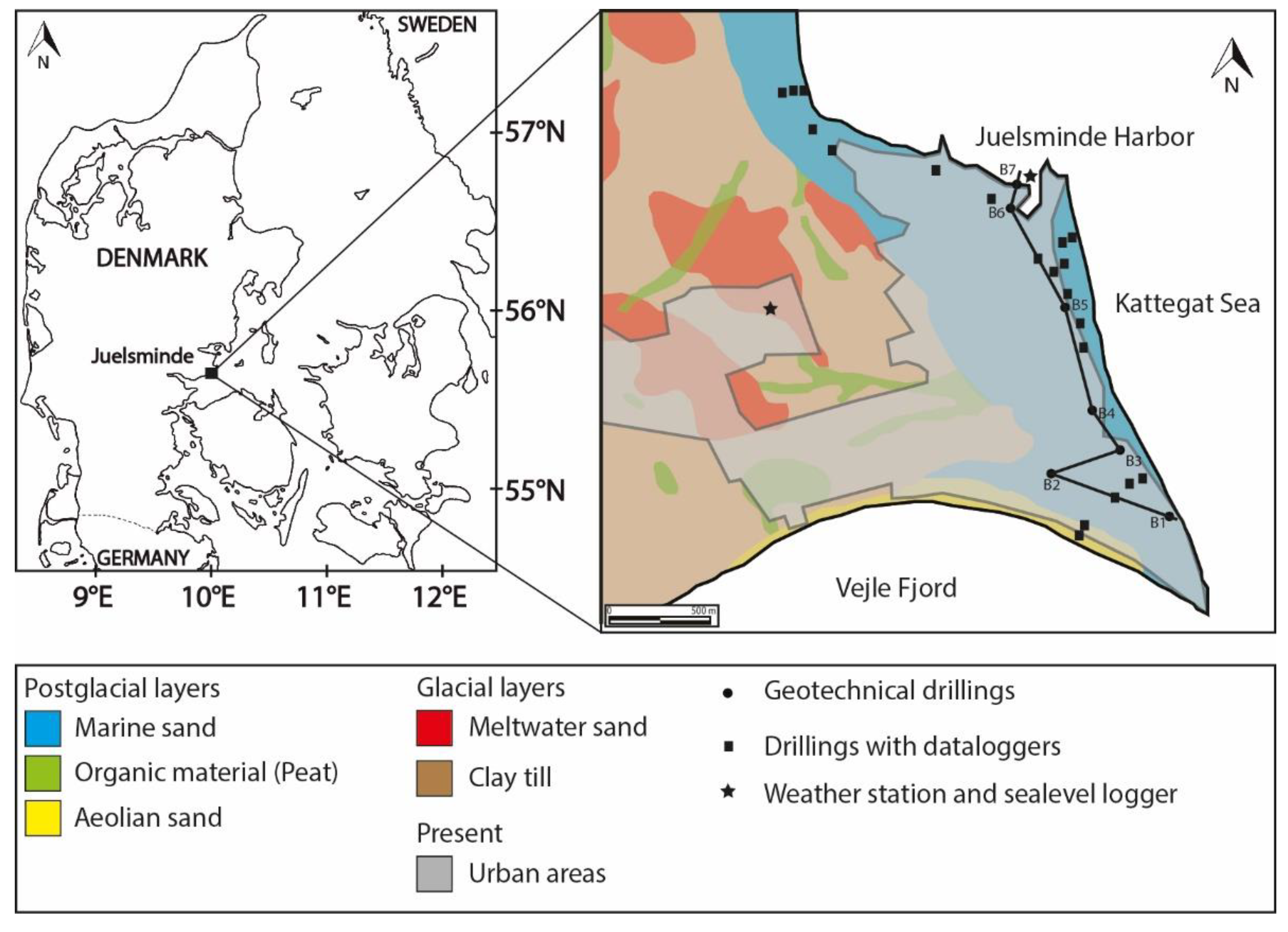
Figure 2.
Cross section through Juelsminde showing borehole lithologies.
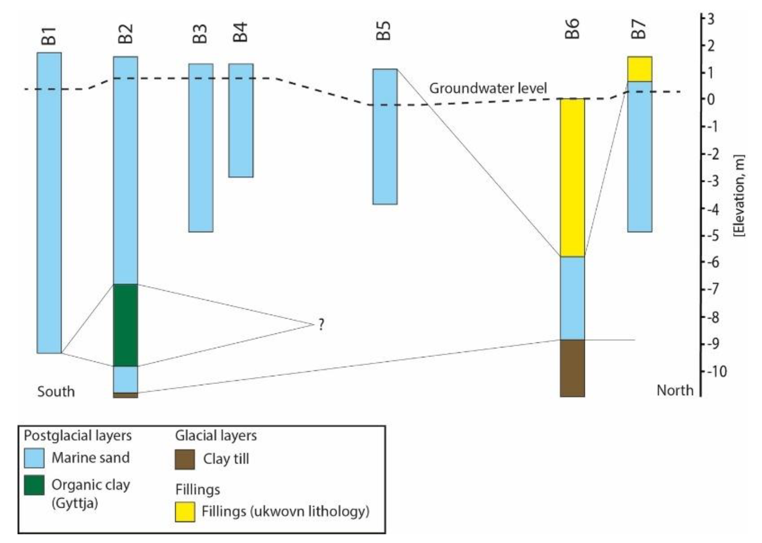
Figure 3.
Location of the different logger types installed in the Juelsminde area.
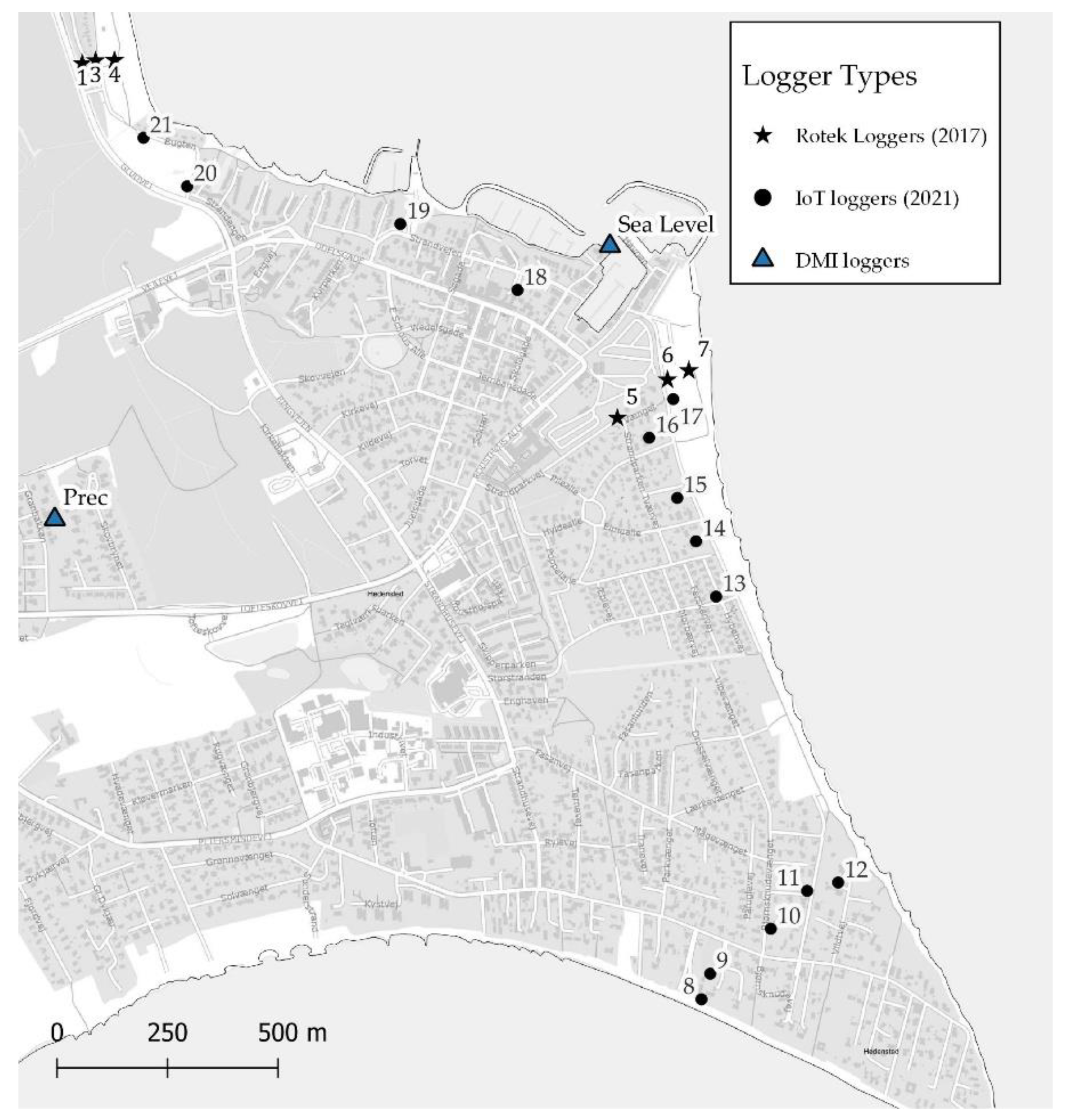
Figure 4.
Workflow of the data treatment, analysis and model process.
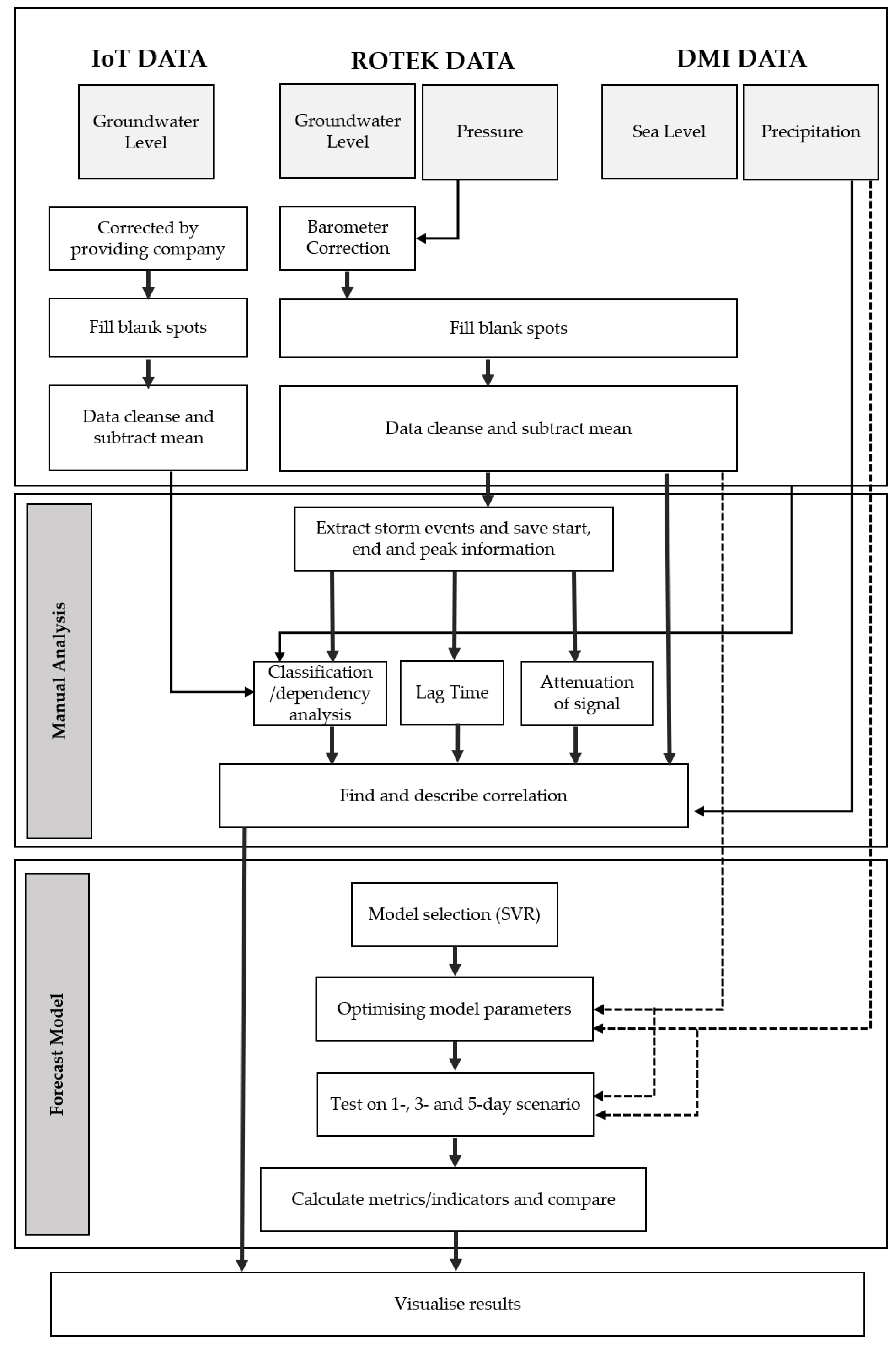
Figure 5.
An example of the automatic selection of high sea level events. The blues crosses representing the peak levels exceeding the the minimum criterias.
Figure 5.
An example of the automatic selection of high sea level events. The blues crosses representing the peak levels exceeding the the minimum criterias.
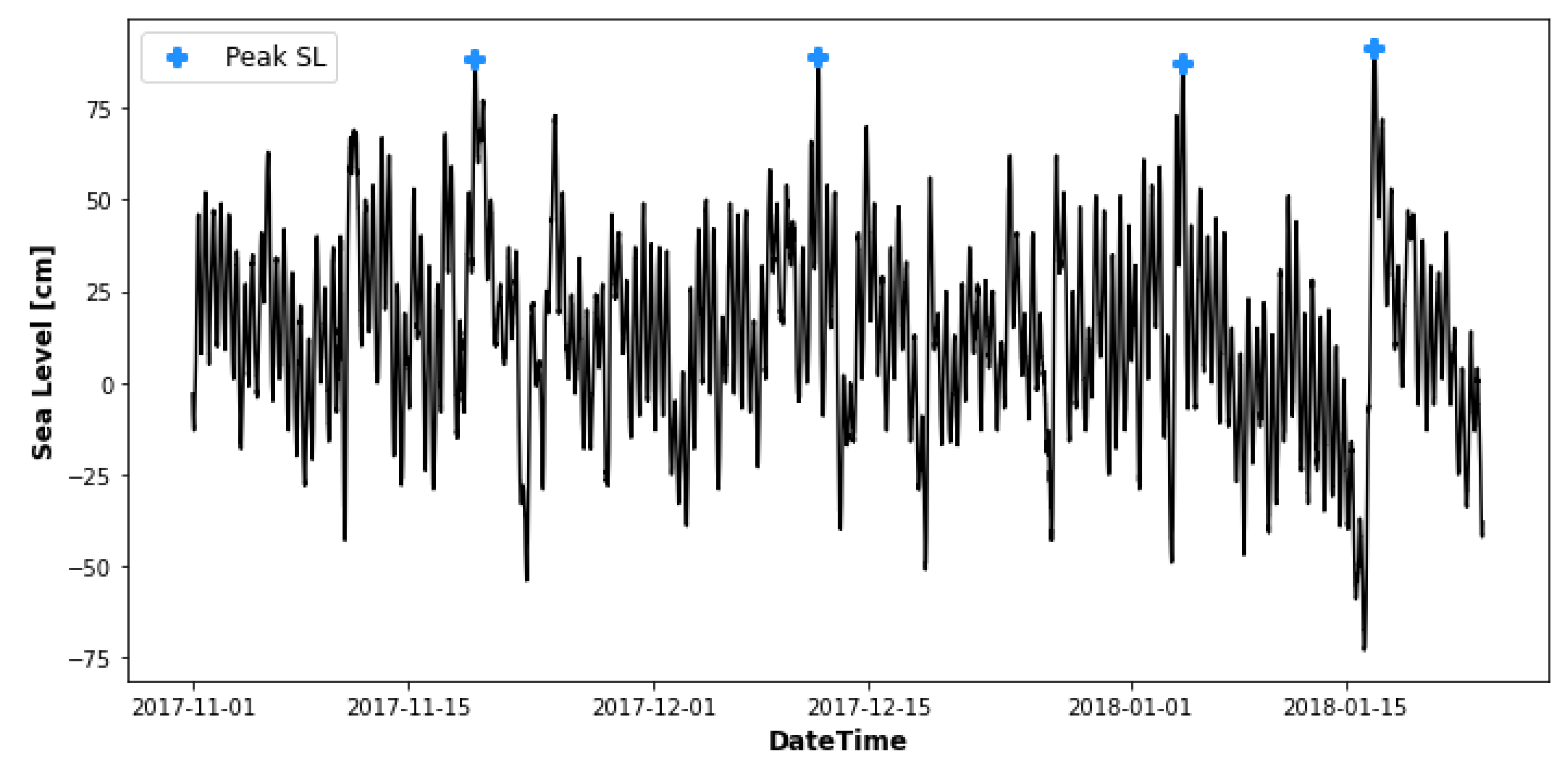
Figure 6.
Boxplot (25% and 75% quartiles) visualising the lag times for the delayed responses in the groundwater table initiated by a sudden rise in sea level in the northern (black) and the southern (grey) profiles.
Figure 6.
Boxplot (25% and 75% quartiles) visualising the lag times for the delayed responses in the groundwater table initiated by a sudden rise in sea level in the northern (black) and the southern (grey) profiles.
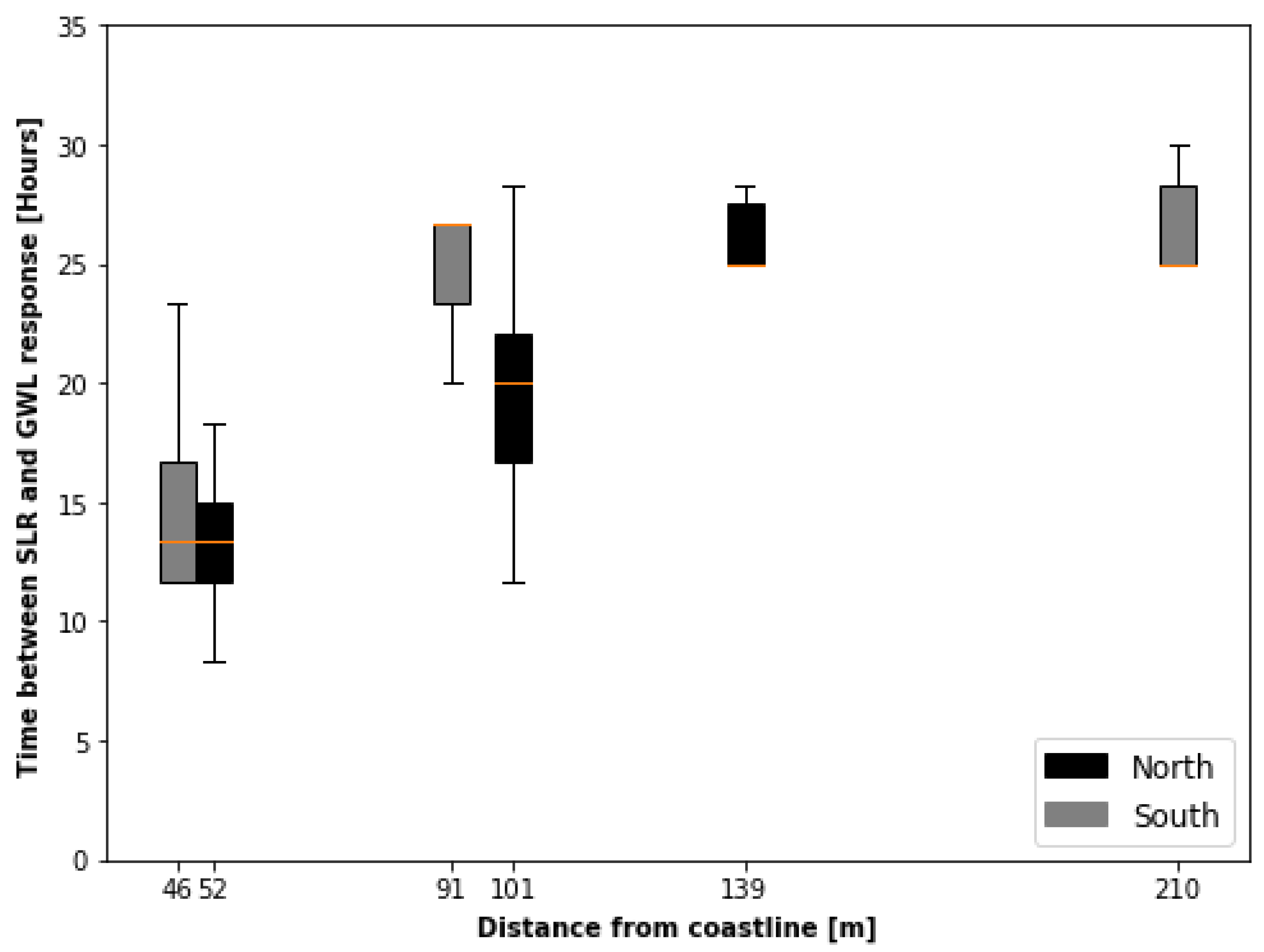
Figure 7.
The relative rise in ground water level monitored in the wells for each of the 30 SLR events.
Figure 7.
The relative rise in ground water level monitored in the wells for each of the 30 SLR events.
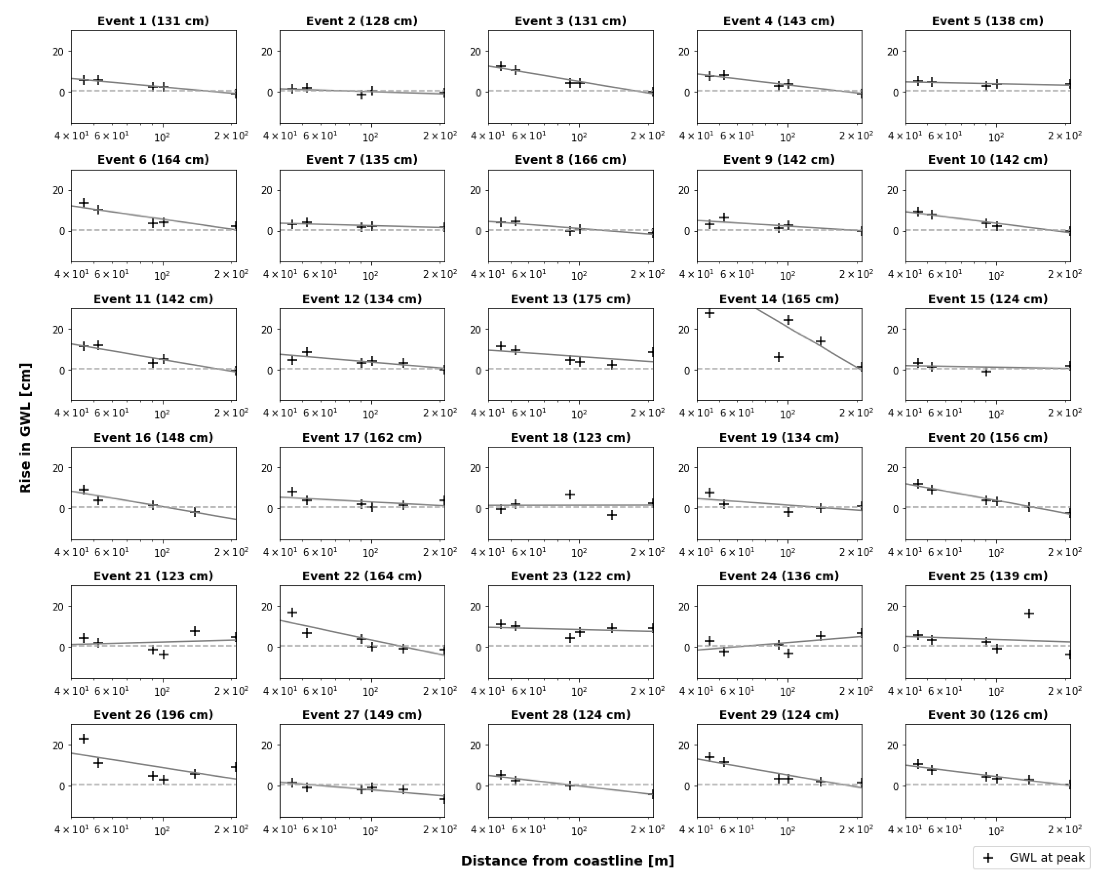
Figure 8.
The relative rise in groundwater level registered in the wells during 30 SLR events.
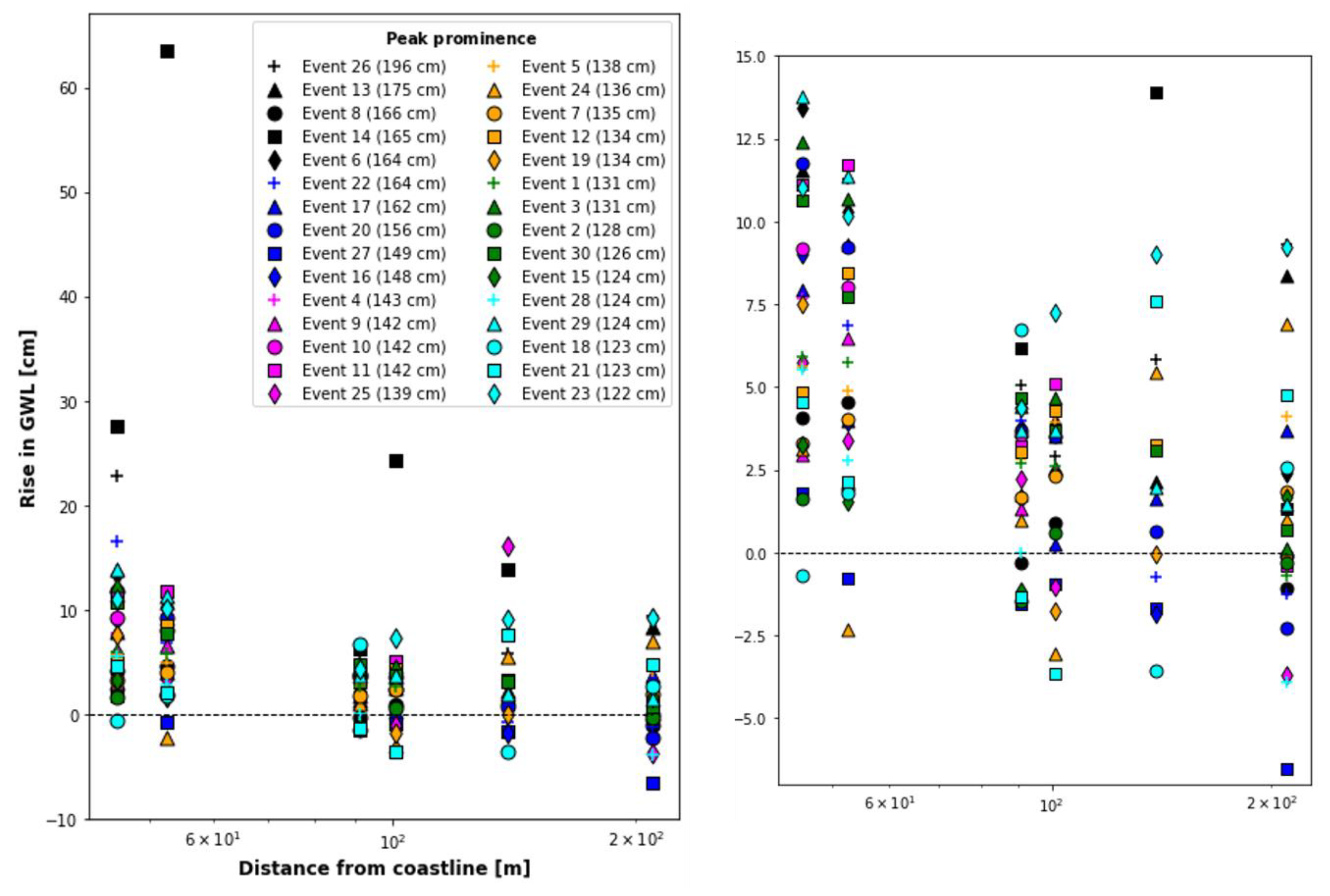
Figure 9.
The relative rise in GWL plotted against the SLR peak prominence for the six wells from 2017.
Figure 9.
The relative rise in GWL plotted against the SLR peak prominence for the six wells from 2017.
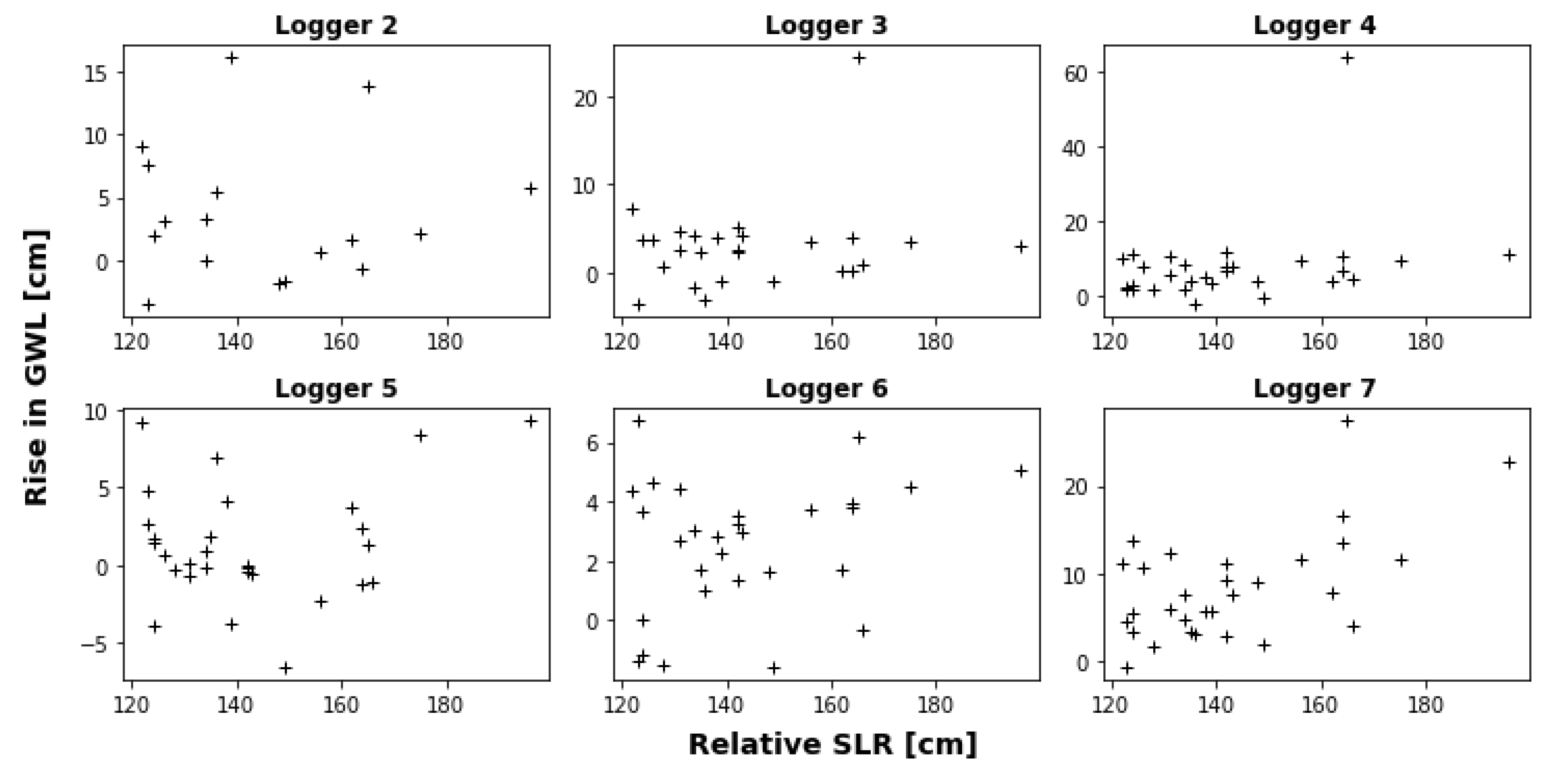
Figure 10.
The classification result for the GWL in each wells dependency of SLR and precipitation events.
Figure 10.
The classification result for the GWL in each wells dependency of SLR and precipitation events.
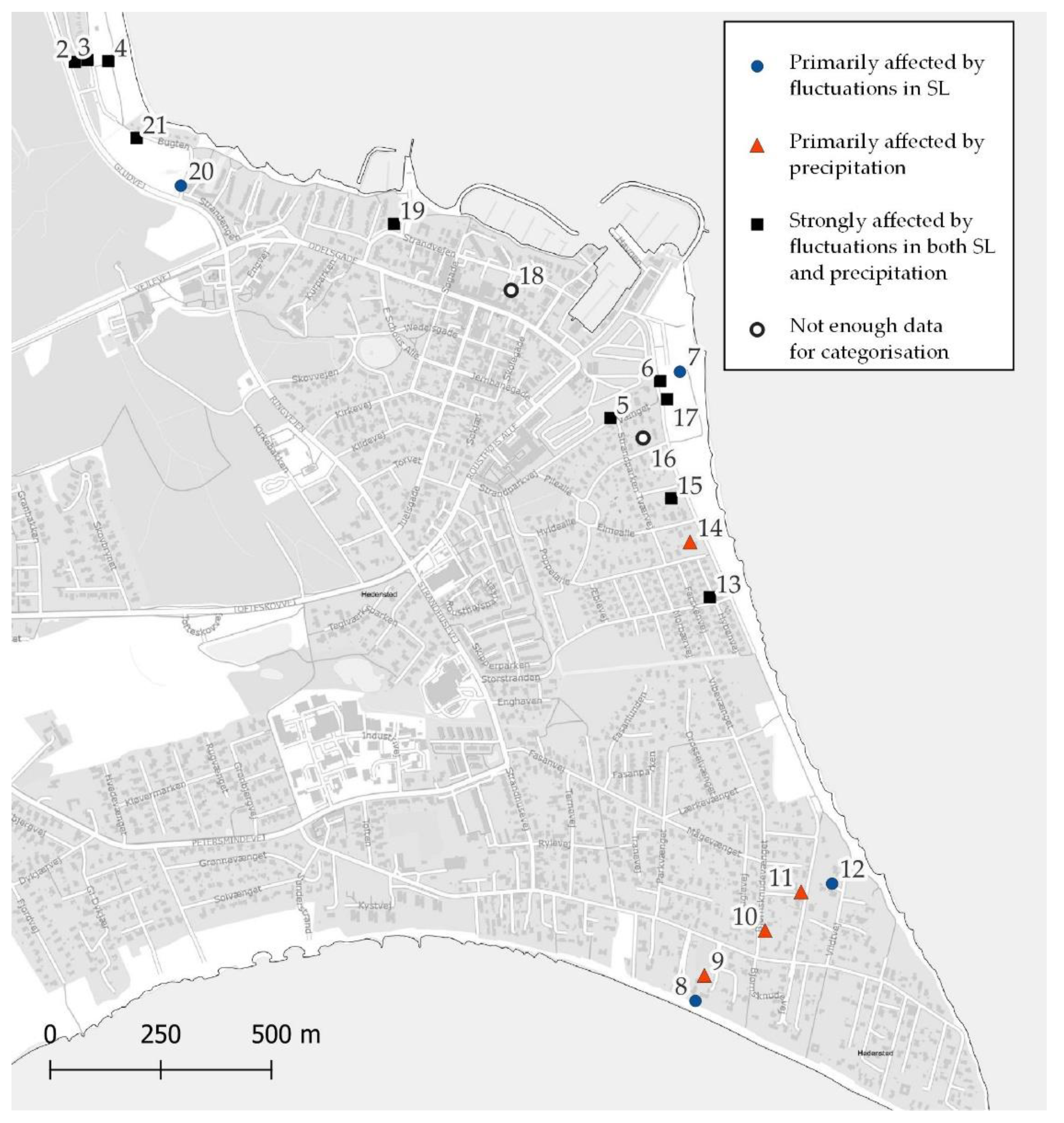
Figure 11.
The modelled and observed GWR in the well 2,3 and 4 during a SLR event.
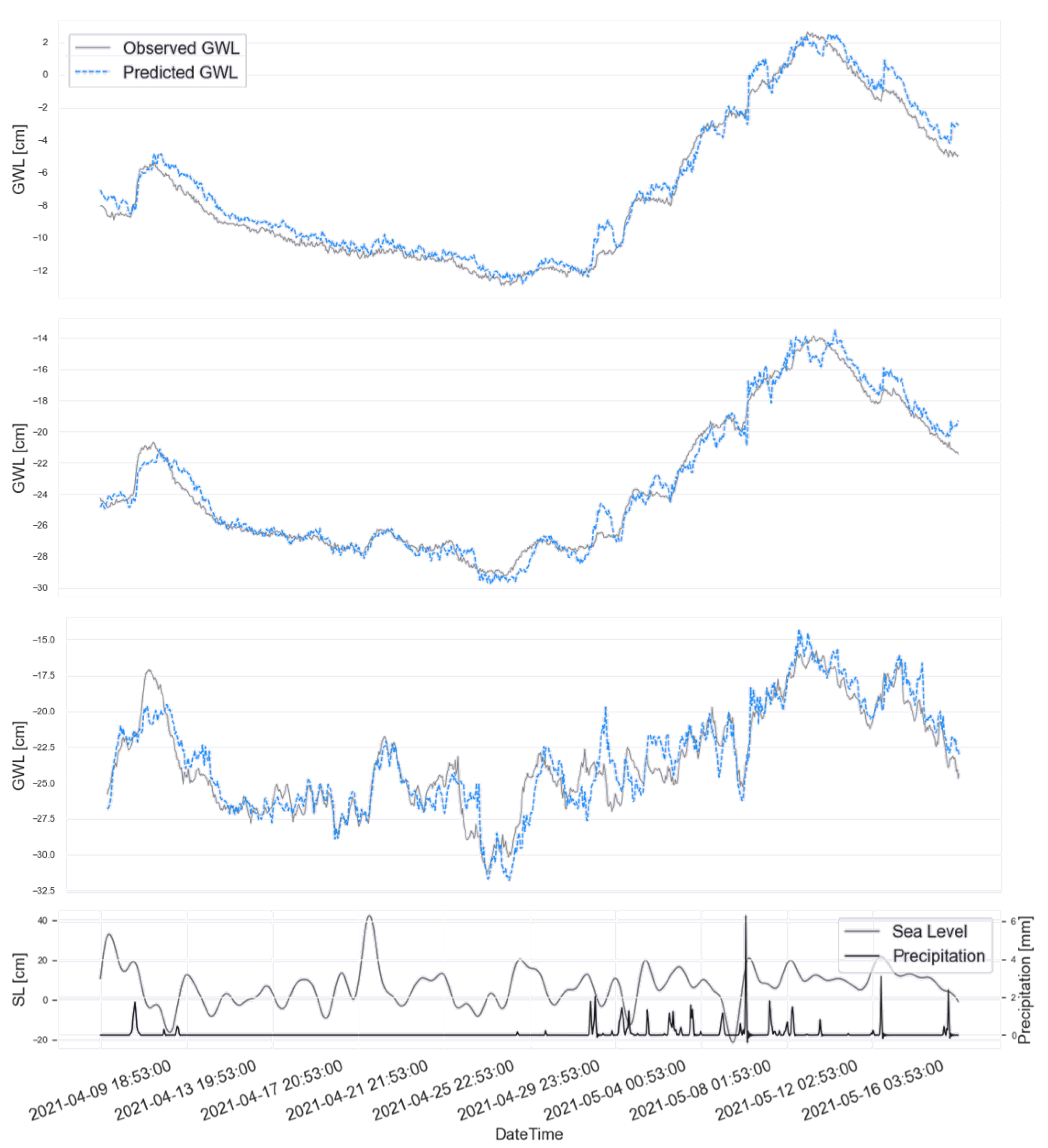
Figure 12.
The modelled and observed GWR in the well 5,6 and 7 during a SLR event.
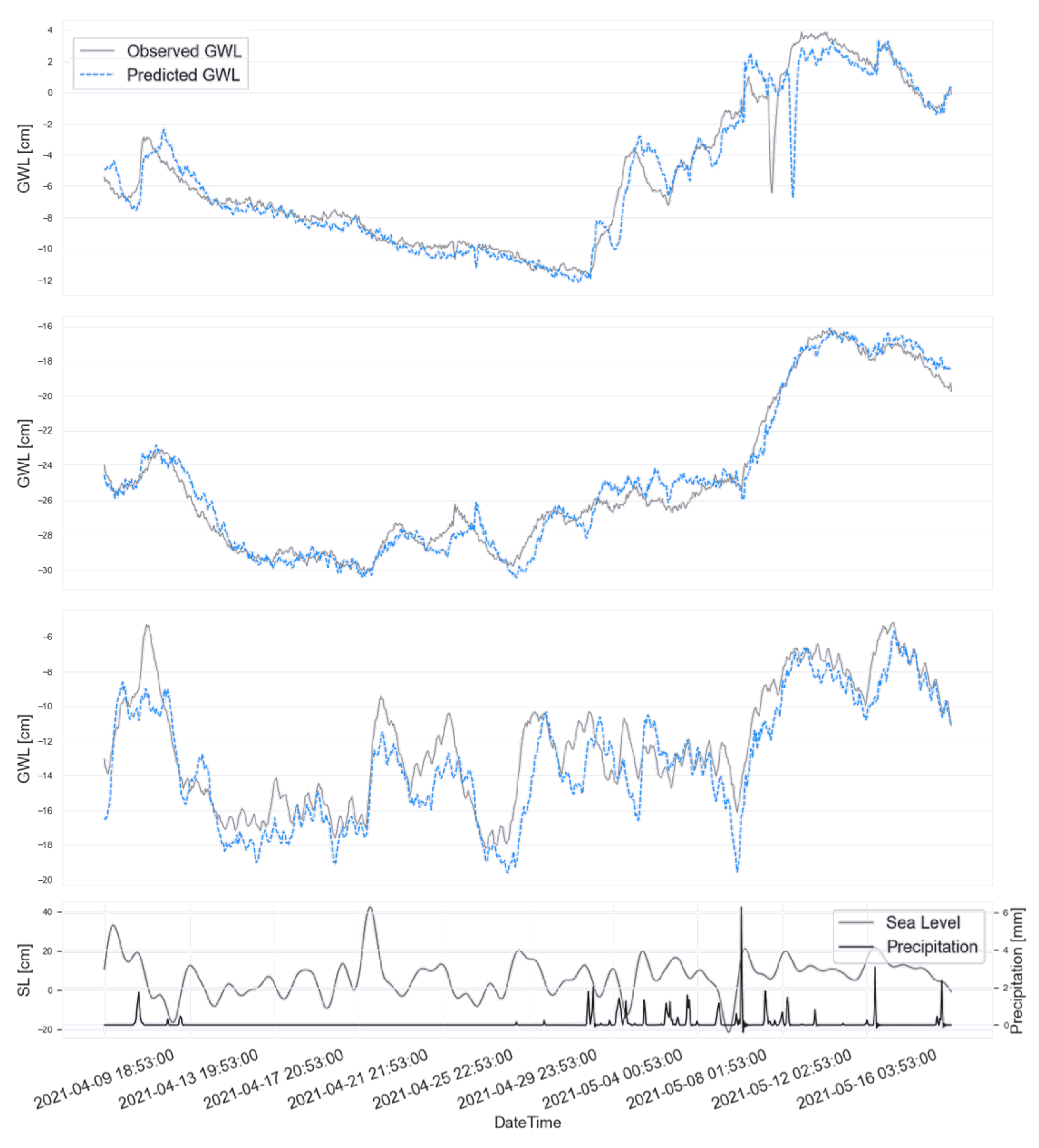

Table 1.
An overview of the data sources used in this study.
| Logger Type | Logger No. | Parameter | LON | LAT | Distance to Coast [m] | Start Time |
|---|---|---|---|---|---|---|
| Rotek loggers |
1 | Barometer | 55,719466 | 9,997424 | 139 | 2017-09-27 |
| 2 | GWL | 55,719519 | 9,997907 | 139 | 2018-08-01 | |
| 3 | GWL | 55,719519 | 9,998589 | 101 | 2017-09-27 | |
| 4 | GWL | 55,712096 | 10,01651 | 52,5 | 2017-09-27 | |
| 5 | GWL | 55,712857 | 10,018334 | 210 | 2017-09-27 | |
| 6 | GWL | 55,713039 | 10,019108 | 91 | 2017-09-27 | |
| 7 | GWL | 55,715592 | 10,016333 | 45,5 | 2017-09-27 | |
| IoT loggers |
8 | GWL | 55,700241 | 10,019238 | 25 | 2021-11-09 |
| 9 | GWL | 55,700759 | 10,019567 | 85 | 2021-11-09 | |
| 10 | GWL | 55,701656 | 10,021771 | 237 | 2021-11-09 | |
| 11 | GWL | 55,702416 | 10,023098 | 166 | 2021-11-09 | |
| 12 | GWL | 55,702576 | 10,024219 | 95 | 2021-11-09 | |
| 13 | GWL | 55,708428 | 10,019977 | 93 | 2021-11-09 | |
| 14 | GWL | 55,70956 | 10,019282 | 93 | 2021-12-07 | |
| 15 | GWL | 55,710447 | 10,018632 | 111 | 2021-12-07 | |
| 16 | GWL | 55,711681 | 10,01765 | 153 | 2021-12-07 | |
| 17 | GWL | 55,712459 | 10,018539 | 90 | 2021-11-10 | |
| 18 | GWL | 55,714725 | 10,012991 | 106 | 2021-11-10 | |
| 19 | GWL | 55,716101 | 10,008804 | 75 | 2021-11-09 | |
| 20 | GWL | 55,716932 | 9,999464 | 122 | 2021-12-07 | |
| 21 | GWL | 55,717932 | 10,001148 | 67 | 2021-12-07 | |
| DMI loggers |
100 | Sea level | 55,7156 | 10,0163 | - | 2017-09-27 |
| 101 | Precipitation | 55,7102 | 9,9962 | - | 2017-09-27 |
Table 2.
The selected SLR events and the corresponding peak values.
| Event No. | Start Datetime | Peak Datetime | End Datetime | PeakProminence | SL at Peak |
|---|---|---|---|---|---|
| 1 | 2017-10-07 20:00:00 | 2017-10-13 02:20:00 | 2017-10-19 18:40:00 | 131 | 79 |
| 2 | 2017-10-13 14:10:00 | 2017-10-18 21:20:00 | 2017-10-25 12:50:00 | 128 | 76 |
| 3 | 2017-11-14 03:40:00 | 2017-11-19 10:00:00 | 2017-11-26 02:20:00 | 131 | 88 |
| 4 | 2017-12-06 11:40:00 | 2017-12-11 17:20:00 | 2017-12-18 10:20:00 | 143 | 89 |
| 5 | 2017-12-30 04:40:00 | 2018-01-04 10:10:00 | 2018-01-11 03:20:00 | 138 | 87 |
| 6 | 2018-01-11 12:00:00 | 2018-01-16 21:10:00 | 2018-01-23 10:40:00 | 164 | 91 |
| 7 | 2018-01-23 12:10:00 | 2018-01-28 20:30:00 | 2018-02-04 10:50:00 | 135 | 74 |
| 8 | 2018-02-07 11:20:00 | 2018-02-12 20:30:00 | 2018-02-19 10:00:00 | 166 | 68 |
| 9 | 2018-02-11 02:00:00 | 2018-02-16 10:20:00 | 2018-02-23 00:40:00 | 142 | 60 |
| 10 | 2018-02-22 16:10:00 | 2018-02-27 20:40:00 | 2018-03-06 14:50:00 | 142 | 60 |
| 11 | 2018-03-11 17:20:00 | 2018-03-16 22:50:00 | 2018-03-23 16:00:00 | 142 | 60 |
| 12 | 2018-11-13 13:30:00 | 2018-11-18 19:30:00 | 2018-11-25 12:10:00 | 134 | 55 |
| 13 | 2018-11-29 14:00:00 | 2018-12-04 20:00:00 | 2018-12-11 12:40:00 | 175 | 109 |
| 14 | 2019-01-03 15:20:00 | 2019-01-08 23:50:00 | 2019-01-15 14:00:00 | 165 | 136 |
| 15 | 2019-01-13 01:30:00 | 2019-01-18 07:40:00 | 2019-01-25 00:10:00 | 124 | 74 |
| 16 | 2019-02-06 04:35:00 | 2019-02-11 15:25:00 | 2019-02-18 03:15:00 | 148 | 79 |
| 17 | 2019-03-03 01:55:00 | 2019-03-08 22:15:00 | 2019-03-15 00:35:00 | 162 | 104 |
| 18 | 2019-03-11 13:05:00 | 2019-03-16 17:45:00 | 2019-03-23 11:45:00 | 123 | 71 |
| 19 | 2019-03-13 13:15:00 | 2019-03-18 20:45:00 | 2019-03-25 11:55:00 | 134 | 76 |
| 20 | 2019-09-10 14:55:00 | 2019-09-15 23:45:00 | 2019-09-22 13:35:00 | 156 | 108 |
| 21 | 2019-10-23 09:35:00 | 2019-10-28 21:05:00 | 2019-11-04 08:15:00 | 123 | 79 |
| 22 | 2019-11-24 11:35:00 | 2019-11-29 11:55:00 | 2019-12-06 10:15:00 | 164 | 111 |
| 23 | 2019-12-02 11:35:00 | 2019-12-07 18:25:00 | 2019-12-14 10:15:00 | 122 | 102 |
| 24 | 2019-12-07 03:35:00 | 2019-12-12 08:15:00 | 2019-12-19 02:15:00 | 136 | 86 |
| 25 | 2020-01-30 07:35:00 | 2020-02-04 19:35:00 | 2020-02-11 06:15:00 | 139 | 93 |
| 26 | 2020-02-04 18:25:00 | 2020-02-10 22:55:00 | 2020-02-16 17:05:00 | 196 | 136 |
| 27 | 2020-02-18 07:45:00 | 2020-02-23 10:05:00 | 2020-03-01 06:25:00 | 149 | 102 |
| 28 | 2020-03-08 18:05:00 | 2020-03-14 01:35:00 | 2020-03-20 16:45:00 | 124 | 79 |
| 29 | 2020-03-24 07:25:00 | 2020-03-29 14:05:00 | 2020-04-05 06:05:00 | 124 | 75 |
| 30 | 2020-09-11 23:15:00 | 2020-09-17 09:15:00 | 2020-09-23 21:55:00 | 126 | 78 |
Table 3.
The main outcomes of the SVR model predictions of the groundwater level 1, 3 and 5 days ahead using data from Logger 4.
Table 3.
The main outcomes of the SVR model predictions of the groundwater level 1, 3 and 5 days ahead using data from Logger 4.
| 1 Day | 3 Days | 5 Days | ||||
|---|---|---|---|---|---|---|
| Average | Std. dev. | Average | Std. dev. | Average | Std. dev. | |
| R2adj | 0.76 | 0.19 | 0.43 | 0.37 | -0.27 | 0.78 |
| R2pred | 0.10 | 0.99 | 0.23 | 0.51 | -0.65 | 1.12 |
| MAE | 1.30 | 0.56 | 3.14 | 1.06 | 4.90 | 1.67 |
| RMSE | 1.99 | 1.07 | 6.94 | 2.45 | 13.02 | 4.29 |
Disclaimer/Publisher’s Note: The statements, opinions and data contained in all publications are solely those of the individual author(s) and contributor(s) and not of MDPI and/or the editor(s). MDPI and/or the editor(s) disclaim responsibility for any injury to people or property resulting from any ideas, methods, instructions or products referred to in the content. |
© 2023 by the authors. Licensee MDPI, Basel, Switzerland. This article is an open access article distributed under the terms and conditions of the Creative Commons Attribution (CC BY) license (http://creativecommons.org/licenses/by/4.0/).
Copyright: This open access article is published under a Creative Commons CC BY 4.0 license, which permit the free download, distribution, and reuse, provided that the author and preprint are cited in any reuse.


