
Submitted:
01 June 2023
Posted:
02 June 2023
You are already at the latest version
Abstract
In Taiwan, peanuts are classified by hand. The kernel quality is judged based on the appearance of peanuts. The identification takes considerable time and labor. Fatigue can induce misrecogni-tion or grade cognition instability due. Peanut defects are generally divided into health, underde-velopment, insect bite, and rupture. This study employed two imaging methods push-boom FX10 and Snapshot. Deep learning was used to detect peanut defects. A push-broom instrument was used for testing. There were 1,560 peanuts, including 240 good and 240 bad ones. There were a total of 1,080 good peanuts and bad peanuts in the test set data, the band selection was used, and a CNN model was built. Based on the results from three methods, 3DCNN could classify with 97%accuracy. The Snapshot was used to achieve the real-time design of a lightweight CNN model. Finally, five bands were selected using PCA, and the screening could be accurate and efficient. The maximum overall accuracy was about 98.5%. Kappa was 97.3% with real-time recognition. This will be a major advantage in the future practical application and commercialization processes. This technique can reduce labor costs, achieve intelligent detection and intelligent grading, and bring breakthroughs to smart agriculture for other crops as well.
Keywords:
Hyperspectral
; Deep Learning
; Peanuts
; Band selection
1. Introduction
Hyperspectral imaging has been recently used in agriculture [1,2] with high accuracy. The drone’s remote sensing accuracy [3] is considerable. The peanut species used in this study is Fabaceae arachis. It is a common agricultural product in Taiwan [4]. It is an essential raw material of edible oil [5]. Peanuts are rich in oil, fat, vitamin A, vitamin B complex, and vitamin E. They contain folic acid and many trace elements like Ca, Fe, and Zn, which are good for humans. Peanuts can be used as raw food or for extracting edible peanut oil, peanut butter, and peanut candies. The quality of peanuts can influence the consumer's health and taste. Peanuts of good quality benefit the consumer's health, whereas those of bad quality have a bad taste. If peanuts are dampened, the consumer may ingest aflatoxin, which harms human bodies. A foreign study on judging peanut maturity through appearance [6] divided peanuts into seven maturity levels. Most existing peanut quality detection machines judge freshly harvested and unprocessed peanuts with low accuracy. Peanuts must be fried before selling. Therefore, this study aims to classify fried peanuts with high accuracy. Peanuts are classified universally by hand-picking in Taiwan, as shown in Figure 1. In the detection phase, the workers judge the kernel quality and class based on appearance and determine whether they are suitable to be sold to consumers for consumption. This method is not objective. The decision is based on the identifier's experience, and eye strain or visual angle may induce misrecognition. This study combined nondestructive hyperspectral imaging with deep learning to improve prediction accuracy. This method could improve prediction accuracy without damaging the peanut’s appearance. Many peanut recognition methods have been proposed recently, but few studies used spectra for peanut shell defect detection and quality analysis. In 2016, Jiang et al. [7] proposed using PCA to identify peanut aflatoxin with 98.7% accuracy. Qi et al. [8] separated healthy peanuts from peanuts with aflatoxin. Han and Gao [9] used control classification before and after infection with aflatoxin with 95% accuracy. Xueming et al. [10] so separated healthy peanuts from peanuts with aflatoxin with 94% accuracy. Liu et al. [11] used Unet and the self-created Hypernet method to search for aflatoxin, and the self-created method was able to single out peanuts with aflatoxin. Qi et al. [8] used an SVM classifier with an accuracy of 98%, which yields the highest accuracy among all the above-mentioned methods. However, when comparing it with the method proposed in this study, the accuracy of the SVM method was lower than expected. Zou et al. [12] used RGB graphs to classify peanut shells’ health and various growth levels with an accuracy of 91.15%. However, they only looked for the fullness of peanut shells and judged the growth of peanuts. Qi et al. [13] used GoogleNet of 2DCNN to search for peanut leaf distribution with an accuracy of 97%. Both methods used 2DCNN, but they did not aim at peanut shells. Therefore, this study proposed a CNN method and focused on analyzing the quality of peanut shells with high accuracy. The above-mentioned research methods and related data are compared in Table 1. With the assistance of peanut farmers in Yuanchang Township of Yunlin County in Taiwan, about 3,000 peanuts were collected to create a database for this study. The peanut processing procedure is shown in Figure 1. A color sorter selected the harvested peanuts. Then these peanuts are manually sorted and packed. This study sorted the tumbled peanuts to screen insect-damaged, underdeveloped, and broken peanuts. The FX10 push-broom camera was used for imaging with a spectral range of 400 nm~1000 nm. The band selection was combined with deep learning for training so that the 3DCNN model can classify peanuts more accurately, With an accuracy of 97%. The push-broom camera takes a long time, and peanuts cannot be instantly sorted. The spectral range of 700 nm~900 nm had the best performance. This study used a Snapshot camera to shoot the peanuts in real-time with a spectral range of 600 nm~1000 nm. The band selection mechanism was used to select five bands and used lightweight 2DCNN as the core of recognition. The real-time (30 FPS) accuracy was 98.5%. Therefore, the hand-picking method can be replaced by a rapid and real-time nondestructive method. Different from other papers, this study used peanut shells instead of peanut kernels for recognition. In the model architecture, only one convolution layer was used to reduce the number of features, and the Group Normalization method was used for convergence with higher accuracy. The proposed method could be combined with robot arms to make a peanut screening machine for the farmers to reduce labor costs in the future. This machine can be applied to other crops, bringing breakthroughs to smart new agriculture.
2. Materials and Methods
2.1. Peanut samples
There are wide varieties of peanuts. The black peanuts having high yield and value in Taiwan were selected. These peanuts are produced in Yuanchang Township, Yunlin County, Taiwan. This study collected healthy, underdeveloped, insect-damaged, and ruptured peanuts. The ruptured peanuts included two classes of peanuts with and without peanut kernels inside. There were only two classes good and bad.
Table 1 shows the peanut quantity data of the FX10 push-broom camera experiment. The training set data is 477 peanuts (237 good peanuts and 240 bad peanuts). The test set data is divided into three batches, and each batch of data contains 180 good peanuts and 180 bad peanuts. The total test set data is 1,080 peanuts. Table 2 shows the peanut quantity data of the Snapshot camera experiment, the training set data is 700 peanuts (350 good peanuts and 350 bad peanuts), and the test set data is 2,700 peanuts.
2.2. Hyperspectral imaging system
The push-broom FX10 and snapshot HSI cameras were used for shooting in this experiment. The FX10 is made by SPECIM Ltd., Finland. The spectral range used in this study was 400–1000 nm. The spatial resolution was 1024x629 with 224 bands. The snapshot HSI camera is made by Belgium Imec. As shown in Figure 3, the wavelength range was 600~1000 nm with 25 bands. The spatial resolution was 216x409. USB communication interface was used. The snapshot HSI camera was more convenient to assemble than the line-scan system with a plug-and-play setting. Furthermore, it can obtain hyperspectral data immediately and analyze spectral differences.
During the FX10 push-broom sampling, the samples were placed on a movable plate and spaced without overlapping. Twelve peanuts were analyzed for each sample. Peanut shooting is arranged as shown in Figure 4. There were six good, and six bad peanuts shot each time. A mobile platform and a correction whiteboard were placed underneath. The shooting was performed in a dark box to prevent interference from other light sources. The spectral range was 400 nm-1000 nm, and 224 spectral images were taken by the hyperspectral camera, with 1024x629x224 resolution.
During the snapshot sampling, the samples were placed on the plate and spaced apart. Four peanuts were analyzed for each sample. Peanut shooting is arranged as shown in Figure 4. Two good and two bad peanuts were shot each time. The correction whiteboard was used before shooting. The spectral range was 600-1000 nm. The hyperspectral camera took 25 images with 216x409x25 resolution.
After obtaining the hyperspectral image, the spectral features of normal, underdevelopment, insect bite, and rupture with/without kernels were drawn, as shown in Figure 5
2.3. Principal Component Analysis (PCA)
In Dunteman’s study [14], the principal component analysis (PCA) is an unsupervised linear transformation technique. The technique proposed by Martinez and Kak [15] is extensively used in different fields, primarily in feature extraction and dimension reduction. The dimension reduction aims to reduce the number of data dimensions maintaining performance. In hyperspectral images [16], PCA is mostly used for band selection.
2.4. Preprocessing
The primary objective of preprocessing is to use a threshold [17] for binarization to segment the background. The background is set as 0 and the position of the peanut is set as 1. The connected component labeling [18] and edge contour [19] detection methods are used for image segmentation. However, the same number of inputs is required with the deep learning model. Therefore, the hyperspectral image of the region of interest (ROI) is resized [20] to unify the ROI images of peanuts. Finally, images were randomly rotated and horizontally and vertically flipped to increase the training data volume and facilitate subsequent training and prediction. The overall process is shown in Figure 7.
2.5. Convolutional Neural Network (CNN)
Present deep learning is one of the largest application domains in machine learning and one of the major tools in AI (Artificial Intelligence). The architecture of a neural network is approximately divided into three parts: input layer, hidden layer or layers, and output layer. The input layer consists of multiple data nodes. Its main function is to input and receive data into the network. The hidden layer intervenes between the input layer and the output layer. There is no standard for the number of hidden layers and the number of neurons in each layer. The optimum number is usually determined by the experimental purpose or results. With an increase in the number of hidden layers the complexity of the problems to be handled increases. However, when there are too many hidden layers, the network is difficult to converge. This may lead to low accuracy or overfitting. Overfitting occurs when training accuracy is high but prediction/validation/test accuracy is low. The output layer computes the result/output. Hyperspectral is a special and emerging imaging technique with high-dimensional characteristics and multiband correlation. In recent years, the hyperspectral image has been extensively used in many areas, such as geology [21], agriculture [22,23], global change [24,25,26], national defense [27], industry [28,29], and food [11,30,31], especially in food quality and safety assessment. The machine learning models based on the images of an FX10 camera and snapshot camera were built respectively in this study. To achieve real-time results, one convolution layer was used with Group Normalization.
2.5.1. 1D-CNN
This study used one-dimensional CNN, and general models were trained using a pixel base. Zhang et al. [32] built a model in 1DCNN and achieved good results in spectral images. Hsieh & Kiang [33] also achieved good results in crops and mixed vegetation. Pang et al. [34] performed rapid viability estimation and prediction of corn seeds in images. Yang et al. [35] performed novel leak detection in oil and gas pipeline systems. Laban et al. [36] performed urban area classification in satellite images. The rough peanuts resulted in signal differences, so the target objects in hyperspectral images were averaged to obtain one-dimensional data. One peanut image was convolved into a pixel using average pooling and trained in the depth model.
2.5.1.1. 1D-CNN model
After removing the background, the images of individual peanuts were convolved into 1 pixel using average pooling before the convolution operation. This study used two convolution layers. The ReLU activation function was used to take 8 and 24 feature maps. Then they were combined using Batch Normalization for convergence. The information was modeled using Flatten layer and imported into the fully connected layer. Finally, SoftMax was used for binary classification. The kernel size was a red frame of 3x1 with a stride of 1 and a batch_size of 10.
Figure 9.
Realtime-1DCNN model.
2.5.1.2. Realtime-1DCNN
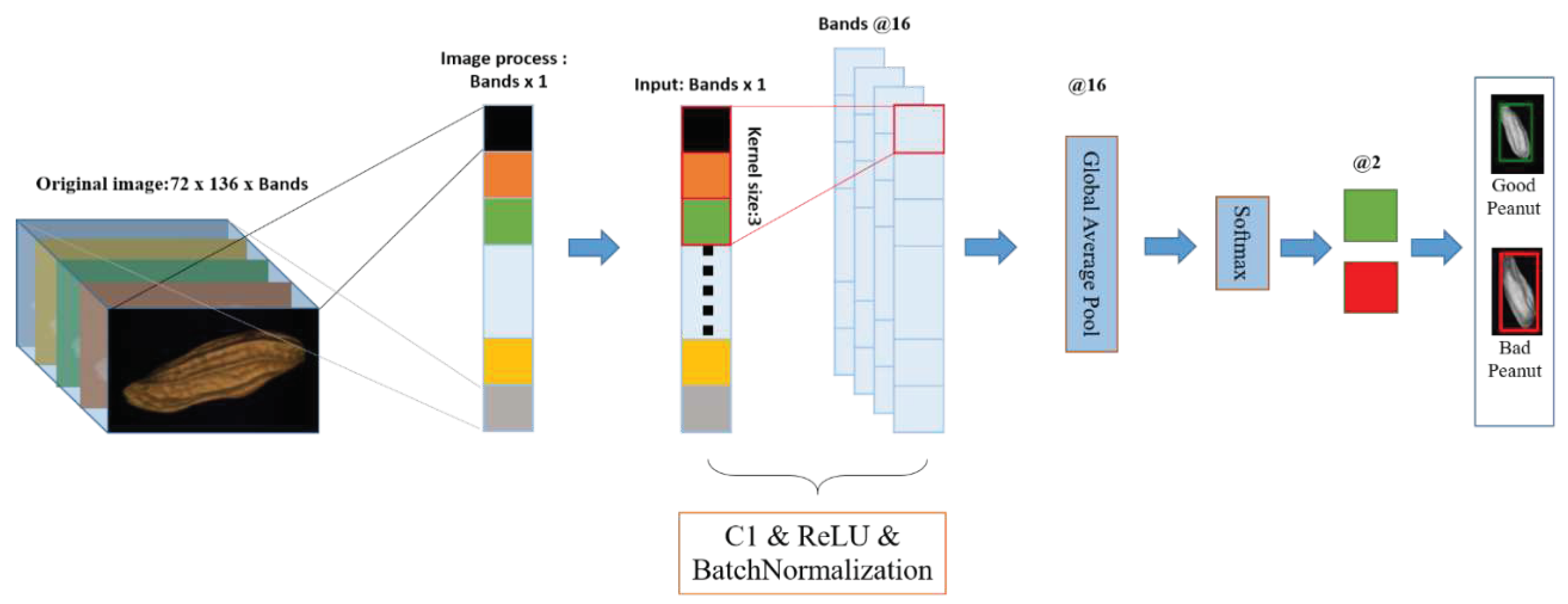
After removing the background, the peanuts were averaged 1 pixel before the convolution operation. This model used one convolutional layer to extract the image features. The activation function was ReLU combined with GroupNormalization. Then the features were averaged using the Global Pooling layer. Finally, the good peanuts and bad peanuts were classified using SoftMax. The kernel size was red frame 3x1 with a step size of 1 and a batch_size of 8.
2.5.2. 2D-CNN
Wang et al. [37] used 2DCNN for detecting water and chlorophyll content in agricultural products and obtained very good results. They prove that the final classification can be influenced by increasing the network depth. The VGG enhances the network classification capacity through deep networks. The number of convolution layers is increased between different layers to enhance the image classification capacity. Rustowicz et al. [38]mentioned that applying 2DCNN to crops has a considerable level. Moreno-Revelo et al. [39] used tens of plant types for classification with good accuracy. Toraman [40] used it for predicting epileptic attacks and identifying ongoing seizures. The VGG-16 and VGG-19 network architectures are the most frequently used. The major advantage is that a moderate network depth can reduce the number of parameters and computing time.
2.5.2.1. 2D-CNN model
As illustrated by the model in Figure 10, the model was trained in 2D. The kernel size used in this model was 3x3 (red frame) with a stride of 1. Three convolution operations with 32, 64, and 128 feature maps were performed. Three Max-Pooling operations were performed to reduce the dimension of the feature maps. One Global Average Pooling operation was used to reduce the dimension of the feature maps. Afterward, two fully connected layers were used, and the good and bad peanuts were classified by using SoftMax. The batch_size was 10.
2.5.2.2. Realtime-2DCNN
As illustrated by the model in Figure 11, the model was trained in 2D. The kernel size was 3x3 (red frame), and the step size was 1. This model used one convolution layer to extract 16 image features with Group Normalization. Then one Global Average Pooling operation was used for the eigenmatrix dimension reduction operation. Finally, the good and bad peanuts were classified using SoftMax. The batch_size was 8.
2.5.3. 3D-CNN
Ji et al. [41] used 3DCNN in airport monitoring. Saveliev et al. [42] obtained a good recognition rate in 3DCNN activity recognition in real-time. The model had the best accuracy with a 3x3x3 kernel. Ji et al. [43,44] used it to recognize a wide range of crops with high accuracy. In the current study, the RandomNormal initialization of Keras was used to obtain better initial values.
2.5.3.1. 3D-CNN model
As illustrated by the model in Figure 12, the model was trained by space and spectrum in 3D. The kernel size was 3x3x3 (red frame), and the step size was 1. Three convolution layers were used to extract image features. The three layers were 4, 16, and 32 feature maps. Two Max-Pooling layers were used to reduce the dimension of the feature maps. Then one layer of Global Average Pooling was used. Finally, the good and bad peanuts were classified using SoftMax with a batch_size of 10.
2.5.3.2. Realtime-3DCNN
As illustrated by the model in Figure 13, the model was trained by space and spectrum in 3D. The kernel size was 3x3x3 (red frame), and the step size was 1. One convolution layer (16 feature maps) was used to extract image features with GroupNormalization. Then one layer of Global Average Pooling was used to reduce the dimension. Finally, the good and bad peanuts were classified using SoftMax with a batch_size of 10.
2.6. Flow chart
The processing procedures of the hyperspectral images captured by FX10 and Snapshot were the same. The dimension of the original data was reduced by PCA band selection, and discriminative spectral information remained. Then the CNN input data were derived from the image by image preprocessing. First, the peanut was separated from the background in the original image. Then the connected component labeling was used to calculate edge contours. As a result, each peanut was segmented into one image and resized. The data augmentation was performed at last (random horizontal and vertical flipping). The preprocessed data were classified using the self-built CNN model, 1DCNN, 2DCNN, and 3DCNN. The complete process and related processing results are shown in Figure 14. The rightmost picture of Figure 14 shows the final classification results. The green frames represent the correctly identified healthy peanuts, the red frames represent the correctly identified defective peanuts, and the unframed ones represent system misidentification.
3. Results
3.1. Band selection results
This section describes the band selection method used in Section 2.3. PCA was used to find bands with obvious differences between defective and good peanuts. The bands selected by the band selection method were visualized. This study used 3, 5, 10, and 20 bands for detection. The number of bands was up to 20 because excessive bands would induce data confusion and replication. Excessive bands could induce difficulties in future automated hardware design. Therefore, the number of bands was controlled within 20. The FX10 and snapshot band selection results are given below.
3.1.1. FX10 hyperspectral image band selection results
The FX10 push-broom camera was used in this section to show the spectral information of peanuts in different states. The selected bands were displayed and visualized by PCA. As shown in Figure 15, the results of band selection were concentrated between 700 and 800 nm. This means that the spectra in the two band ranges were most effective. Table 4 lists the representative 20, 10, 5, and 3 bands selected by PCA.
3.1.2. Snapshot band selection results
Figure 16 shows the spectral information of different types of peanuts captured by the snapshot camera. The discriminative bands were selected by PCA and visualization. As shown in Figure 16, the bands selected by the PCA method were concentrated between 750 and 1000 nm, meaning the largest difference between the features of healthy and defective peanuts was in the band range. Table 5 lists the 20, 10, 5, and 3 bands selected by PCA as the basis of subsequent processing and analyzes which bands were the most discriminative.
3.2. Classification results flow
3.2.1. FX10 data
The specific ROI of peanuts was segmented from the hyperspectral image of peanuts taken by the FX10 push-broom hyperspectral camera, and then the good and bad ones were classified. Finally, the predicted results were displayed in pseudo-color images. Figure 17 shows the image of a general RGB camera. In this image, the upper six peanuts are healthy, while the lower six are abnormally developed and ruptured peanuts. The healthy and defective peanuts are represented by green and red frames, respectively. Whereas, misjudged peanuts are unframed. Figure 18 shows an experimental image example. There were 20, 10, 5, and 3 bands selected by all band and PCA band selection methods. These were combined with FX10-1D-CNN, FX10-2D-CNN, FX10-3D-CNN, Hypernet [11], Snapshot-1D-CNN, Snapshot-2D-CNN, and Snapshot-3D-CNN for classification, and the results were displayed.
Figure 17.
The upper six are good peanuts, and the lower six are bad peanuts in the peanut RGB image.
Figure 17.
The upper six are good peanuts, and the lower six are bad peanuts in the peanut RGB image.
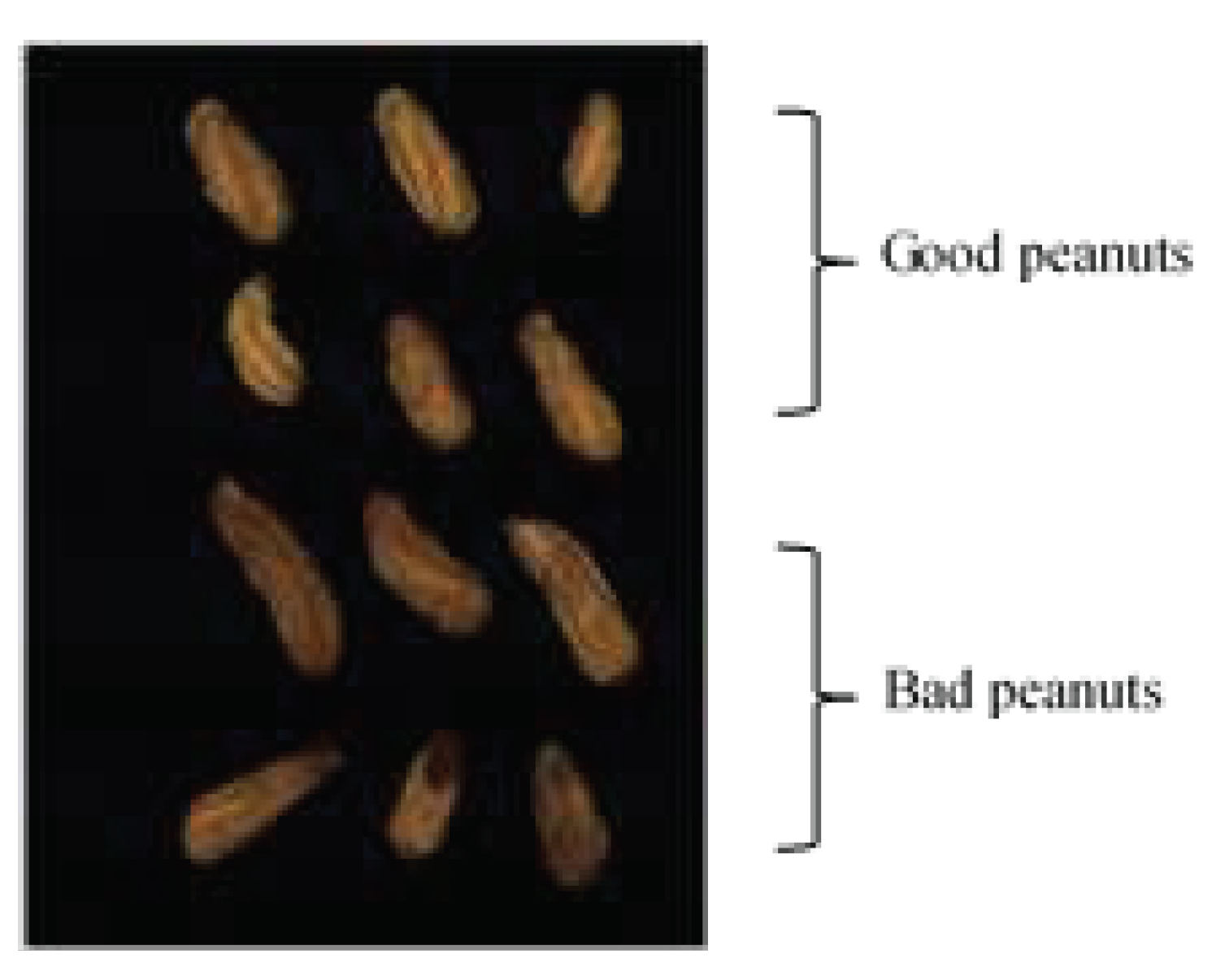
Figure 18.
All band results of peanuts. Green represents healthy peanuts, Red represents defective peanuts, and Unframed peanuts represent misrecognition.
Figure 18.
All band results of peanuts. Green represents healthy peanuts, Red represents defective peanuts, and Unframed peanuts represent misrecognition.
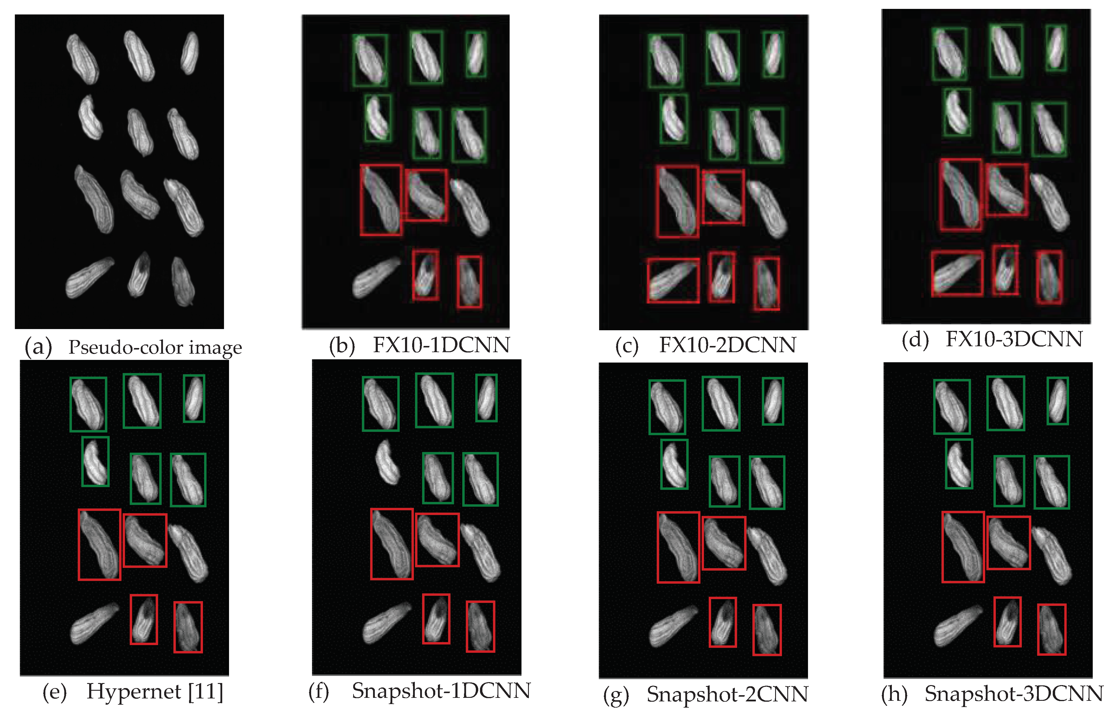
Figure 19.
Classification results of 20 bands. Green represents healthy peanuts, Red represents defective peanuts, and the unframed peanuts represent misrecognition.
Figure 19.
Classification results of 20 bands. Green represents healthy peanuts, Red represents defective peanuts, and the unframed peanuts represent misrecognition.
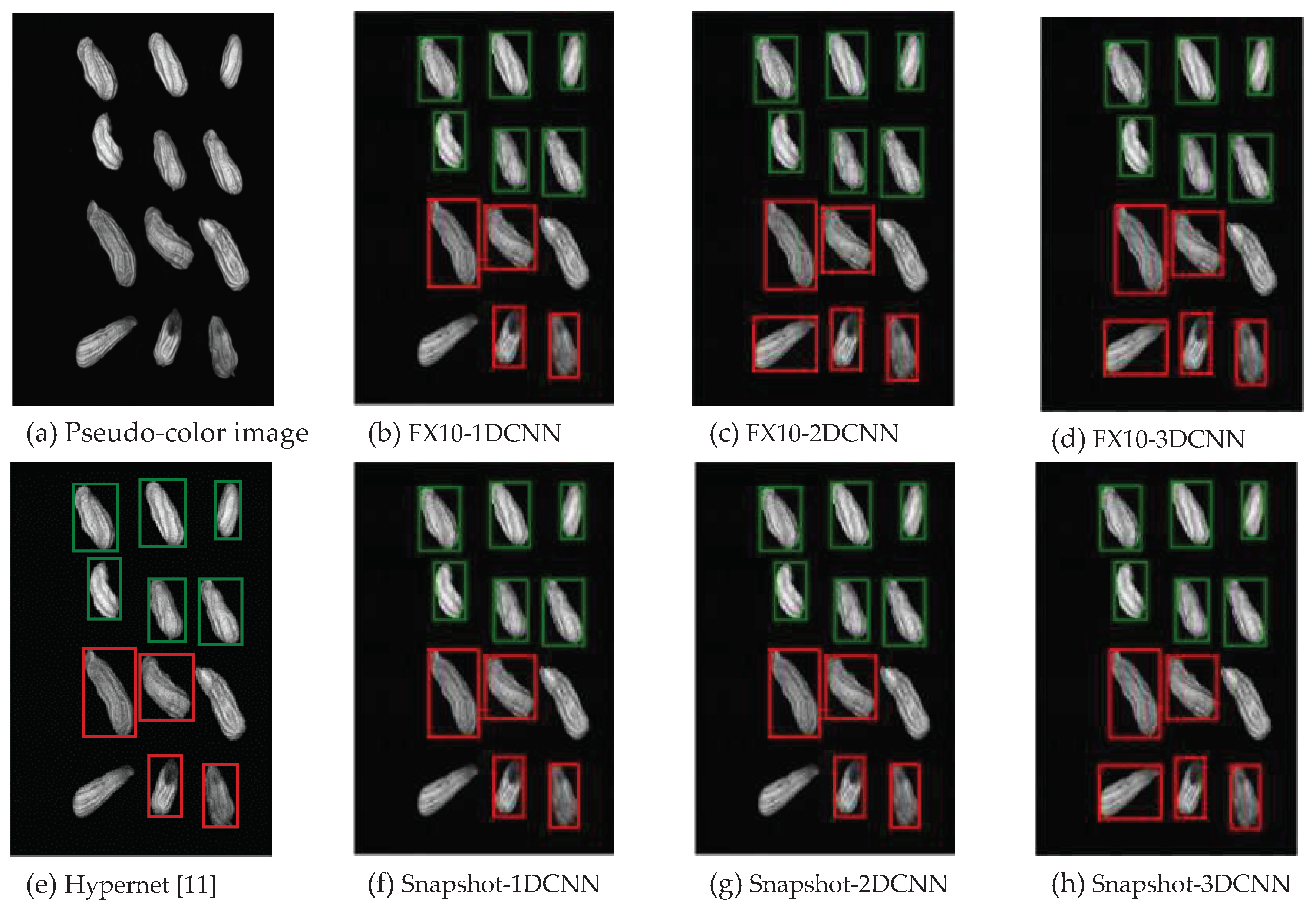
Figure 20.
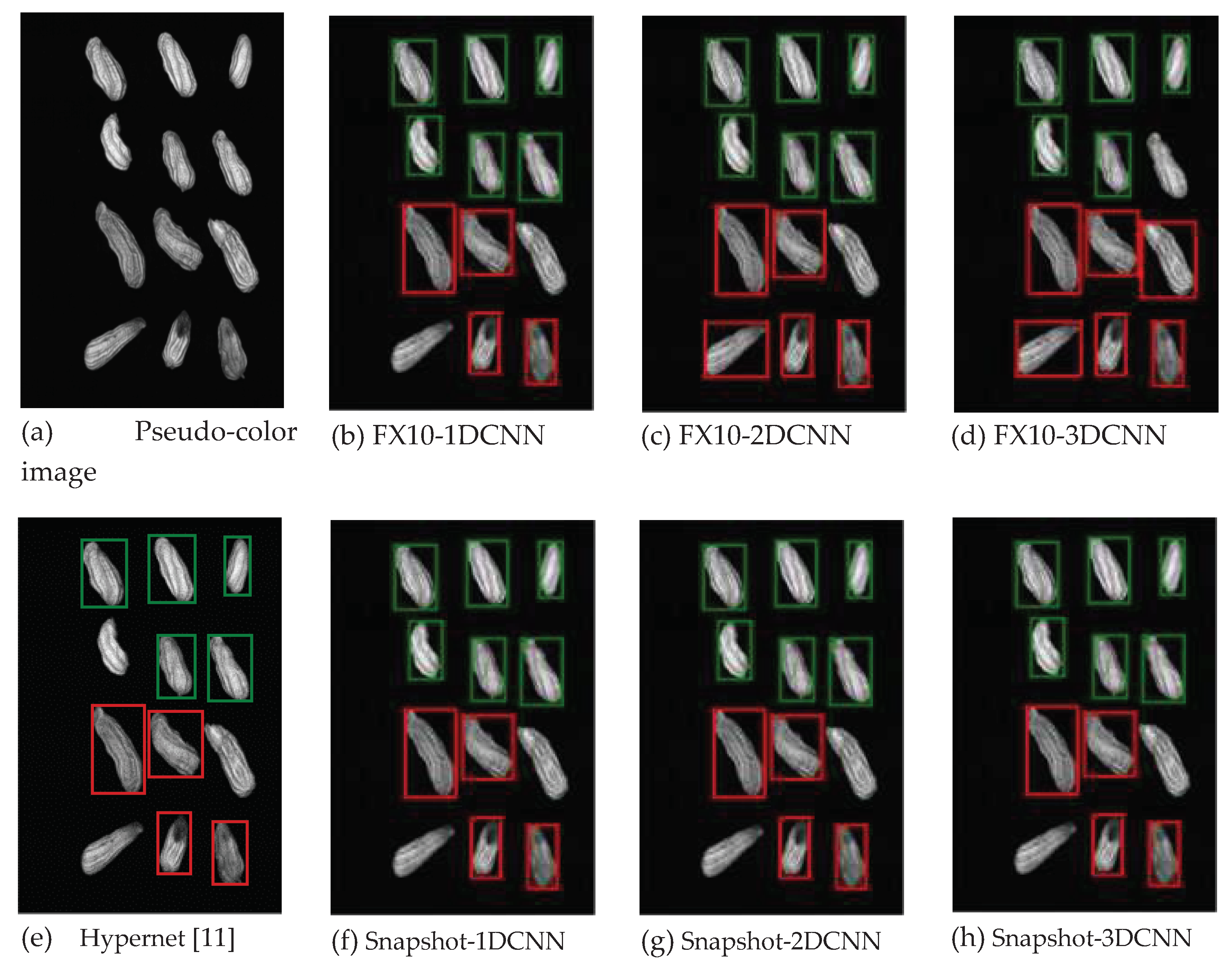
Classification results of 10 bands. Green represents healthy peanuts, Red represents defective peanuts. The unframed peanuts represent misrecognition.
Figure 20.
Classification results of 10 bands. Green represents healthy peanuts, Red represents defective peanuts. The unframed peanuts represent misrecognition.
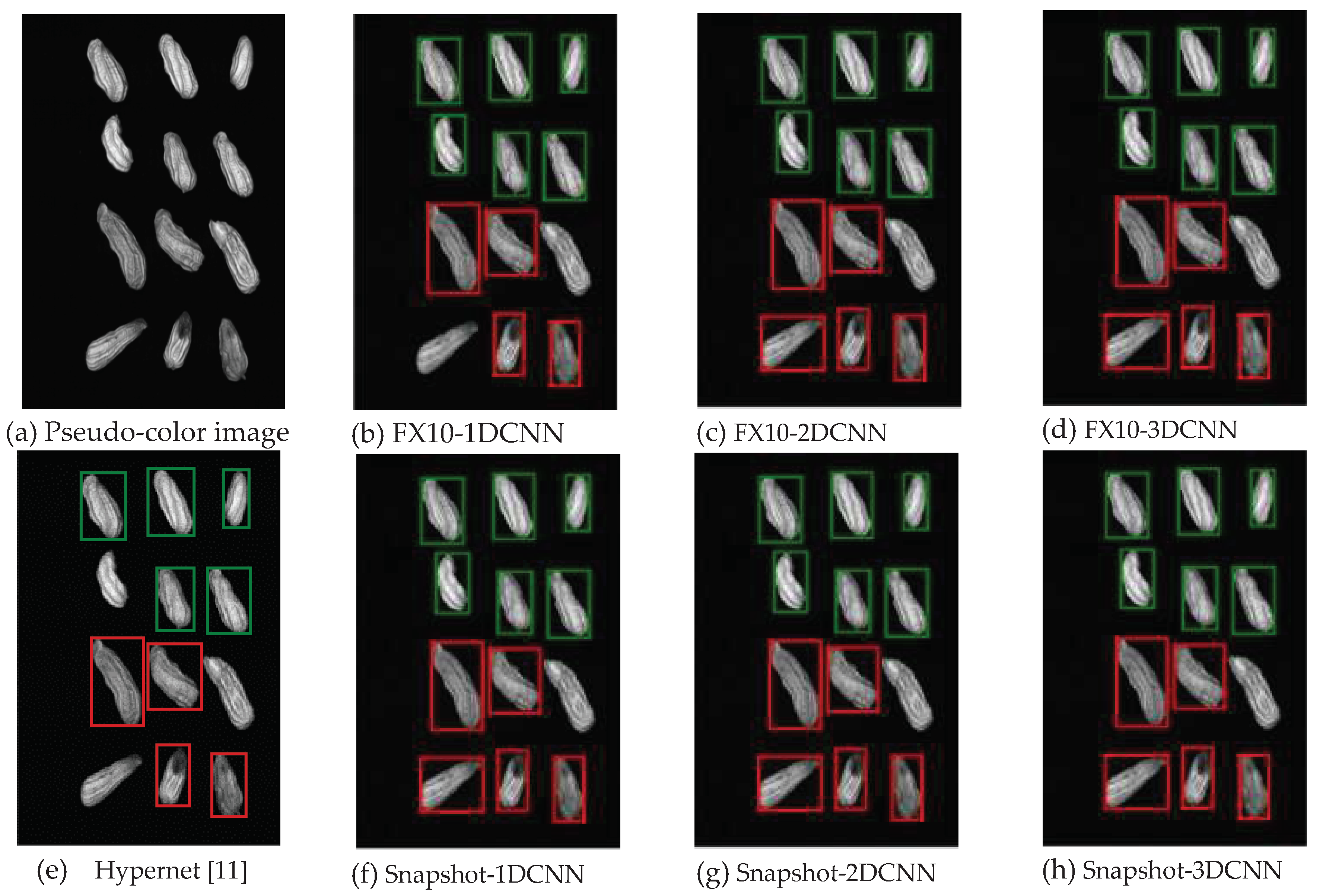
Figure 21.
Classification results of 5 bands. Green represents healthy peanuts, Red represents defective peanuts. Unframed peanuts represent misrecognition.
Figure 21.
Classification results of 5 bands. Green represents healthy peanuts, Red represents defective peanuts. Unframed peanuts represent misrecognition.
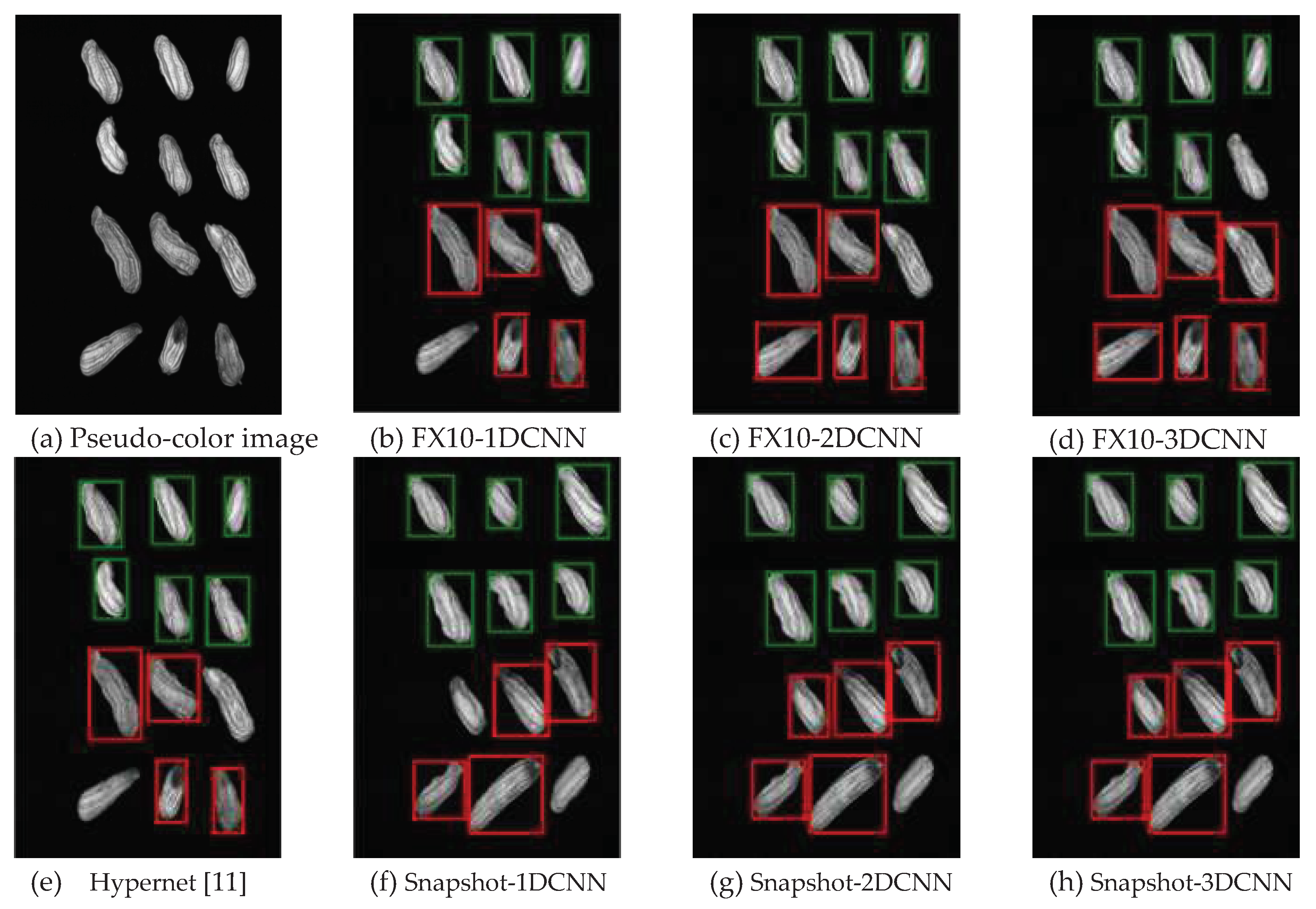
Figure 22.
Classification results of 3 bands. Green represents healthy peanuts, Red represents defective peanuts. The unframed peanuts represent misrecognition.
Figure 22.
Classification results of 3 bands. Green represents healthy peanuts, Red represents defective peanuts. The unframed peanuts represent misrecognition.
3.2.1.Snapshot data
The hyperspectral image of peanuts was obtained using the snapshot hyperspectral camera. The ROI of each peanut was segmented. Then the good and bad ones were classified. Finally, the predicted results were displayed in a pseudo-color image. Figure 23 shows the image taken by a general RGB camera. The two peanuts on the left are normally developed healthy peanuts, and the two on the right are abnormally developed ruptured peanuts. The healthy peanuts are represented by green frames in the recognition result. The defective peanuts are represented by red frames. The unframed peanuts represent misrecognition. The classification result examples of 20 bands (Figure 25), 10 bands (Figure 26), 5 bands (Figure 27), and 3 bands (Figure 28) selected by all bands (Figure 24) and PCA band selection methods with FX10-1D-CNN, FX10-2D-CNN, FX10-3D-CNN, Hypernet [11], Snapshot-1D-CNN, Snapshot-2D-CNN, and Snapshot-3D-CNN are given below.
| Model | Number of bands | TPR | FPR | Acc | Kappa | Runtime(ms) |
| 1D-CNN | Full band | 0.971 | 0.098 | 0.933 | 0.867 | 23.9 |
| 20 band | 0.919 | 0.086 | 0.917 | 0.833 | 23.5 | |
| 10 band | 0.915 | 0.126 | 0.893 | 0.787 | 23.4 | |
| 5 band | 0.933 | 0.145 | 0.890 | 0.780 | 23.3 | |
| 3 band | 0.931 | 0.222 | 0.837 | 0.673 | 23.3 | |
| 2D-CNN | Full band | 0.991 | 0.036 | 0.977 | 0.954 | 30.7 |
| 20 band | 0.997 | 0.047 | 0.974 | 0.949 | 29.4 | |
| 10 band | 0.994 | 0.025 | 0.982 | 0.969 | 27.8 | |
| 5 band | 0.980 | 0.028 | 0.976 | 0.951 | 26 | |
| 3 band | 0.988 | 0.025 | 0.981 | 0.963 | 25.5 | |
| 3D-CNN | Full band | 0.976 | 0.066 | 0.954 | 0.909 | 47.1 |
| 20 band | 0.968 | 0.064 | 0.951 | 0.903 | 33.1 | |
| 10 band | 0.962 | 0.067 | 0.947 | 0.894 | 31.3 | |
| 5 band | 0.971 | 0.050 | 0.960 | 0.920 | 29.6 | |
| 3 band | 0.980 | 0.042 | 0.969 | 0.937 | 28.7 | |
| Hypernet [11] | Full band | 0.930 | 0.021 | 0.953 | 0.906 | 33 |
| 20 band | 0.979 | 0.050 | 0.964 | 0.929 | 31.5 | |
| 10 band | 0.997 | 0.072 | 0.960 | 0.920 | 30.4 | |
| 5 band | 0.979 | 0.047 | 0.966 | 0.931 | 26.5 | |
| 3 band | 0.939 | 0.038 | 0.950 | 0.900 | 24.7 | |
| Realtime-1DCNN | Full band | 0.92 | 0.17 | 0.86 | 0.73 | 23.8 |
| 20 band | 0.907 | 0.269 | 0.793 | 0.586 | 23.4 | |
| 10 band | 0.871 | 0.169 | 0.850 | 0.700 | 23.2 | |
| 5 band | 0.98 | 0.08 | 0.96 | 0.91 | 23 | |
| 3 band | 0.880 | 0.090 | 0.930 | 0.870 | 22.8 | |
| Realtime-2DCNN | Full band | 0.990 | 0.037 | 0.977 | 0.954 | 29.1 |
| 20 band | 1.000 | 0.031 | 0.984 | 0.969 | 28.3 | |
| 10 band | 1.000 | 0.033 | 0.983 | 0.965 | 25.9 | |
| 5 band | 1.000 | 0.031 | 0.985 | 0.973 | 24.8 | |
| 3 band | 0.980 | 0.045 | 0.967 | 0.934 | 24.2 | |
| Realtime-3DCNN | Full band | 0.996 | 0.187 | 0.884 | 0.769 | 28.4 |
| 20 band | 0.948 | 0.073 | 0.937 | 0.874 | 27.9 | |
| 10 band | 0.997 | 0.077 | 0.957 | 0.914 | 26.9 | |
| 5 band | 0.985 | 0.060 | 0.961 | 0.922 | 26.3 | |
| 3 band | 0.988 | 0.050 | 0.969 | 0.937 | 24.4 |
4. Discussion
4.1. Data analysis
This study aims to find the differences between the methods suggested in other literature and the current study and to compare the differences between the results of full band and PCA selected bands. For this purpose, the Kappa, ACC, and time parameters were used for comparison, and the data were displayed in histograms. It was obvious that the Kappa and ACC of FX10 imaging data using the self-developed 3DCNN model were better than other methods. However, the FX10 is very slow in imaging and cannot be applied to production lines. To achieve a high detection rate in the production lines, this study used SnapShot for imaging. To increase the overall speed, this study built a real-time-2DCNN classification model. Based on the accuracy and processing time, the real-time-2DCNN was better than 3DCNN. The detection speed of an image with four peanuts could reach 40 (FPS).
4.1.1. FX10 Data
In the full band condition, the 1DCNN has a better prediction speed but low accuracy than the other two CNN models. However, this problem was solved after band selection. The 1DCNN performs an average operation for the target object so that the target object loses spatial information; only spectral information is used. In the spectral information, the full band is doped with many bands that can cause classification interference and induce misrecognition. Therefore, 20 bands selected by PCA were used as source data, achieving good accuracy. Based on the results, the 1DCNN had the best accuracy with 20 bands. The accuracy slightly decreased with 10 and 5 bands. This means that there might be some important bands influencing the peanut quality discrimination between 10 and 20 bands. The 2DCNN had the second-highest accuracy in this study. A good classification effect could be obtained with a full band. The accuracy of 2DCNN was only maintained at about 96%, possibly because only the spatial information was considered while the information advantage of multiple bands was absent. The advantage of 2DCNN is speed. While it was not as fast as 1DCNN but it was several times faster than 3DCNN. Furthermore, it had the steadiest accuracy among the three models. The 3DCNN had the highest accuracy in FX10 data, but the 3DCNN was not as good as expected with a full band. This might be because the 3DCNN considered spatial information and multiple spectral information simultaneously. The accuracy increased when the PCA was used to select 20 meaningful bands for 3DCNN classification. However, the defect of 3DCNN was that its computing time was higher than 2DCNN. This problem might be solved by reducing the number of bands. A better classification accuracy could be obtained using 3DCNN, disregarding the time cost. Realtime-CNN model’s accuracy was not higher than the original CNN. This might be because the realtime-CNN only used one convolution layer, leading to insufficient features or a lack of higher-level and more complex features.
Figure 29.
FX10 camera hyperspectral ACC histogram.
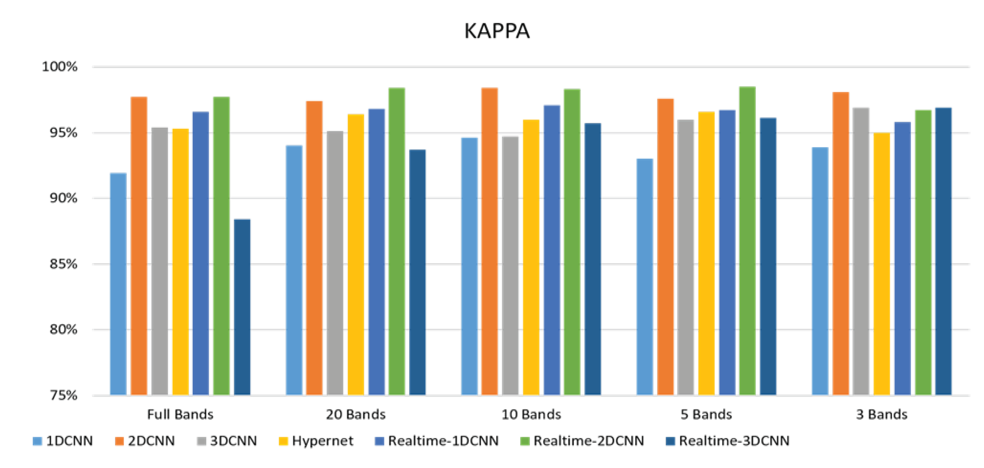
Figure 30.
FX10 camera hyperspectral KAPPA histogram.
4.1.2. FX10 Data
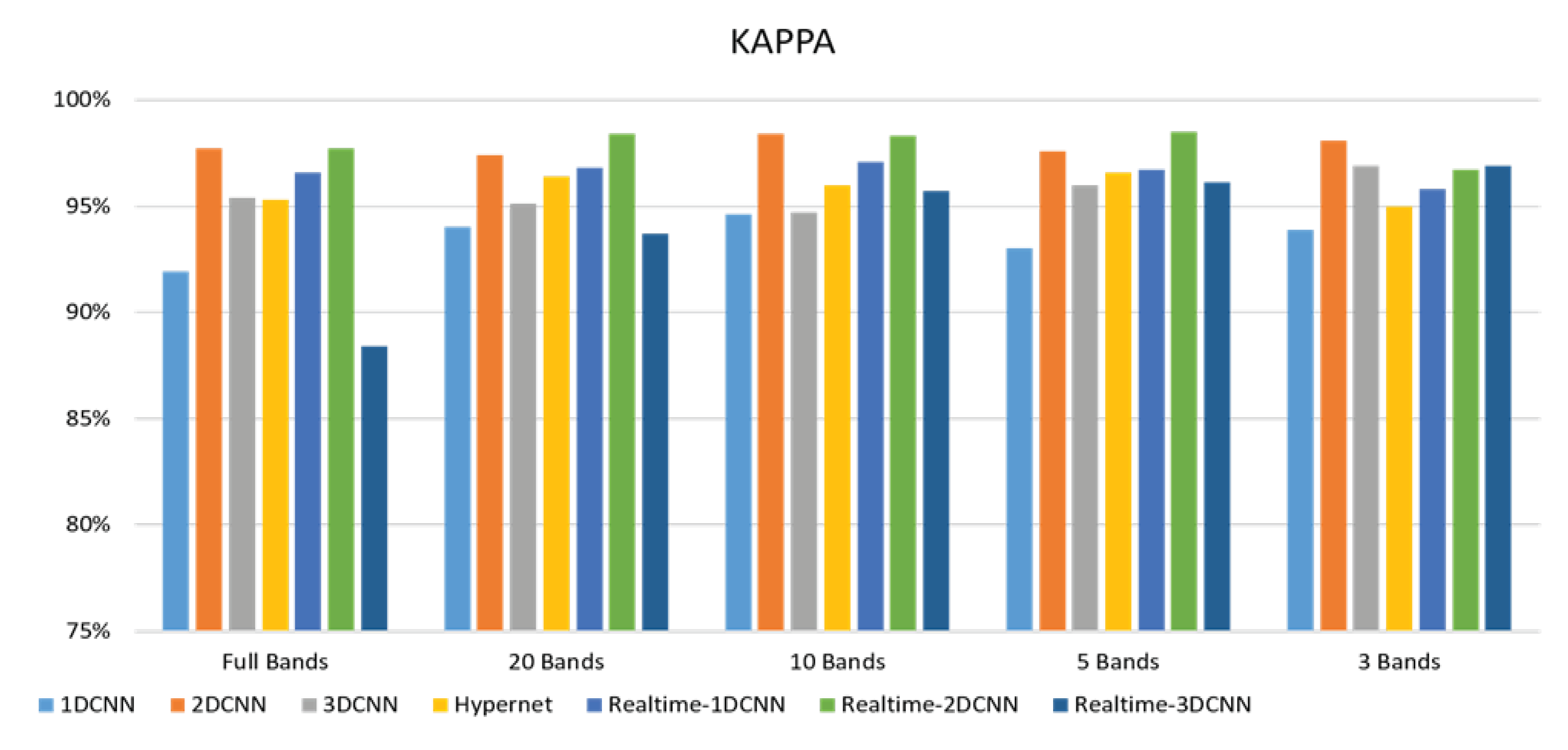
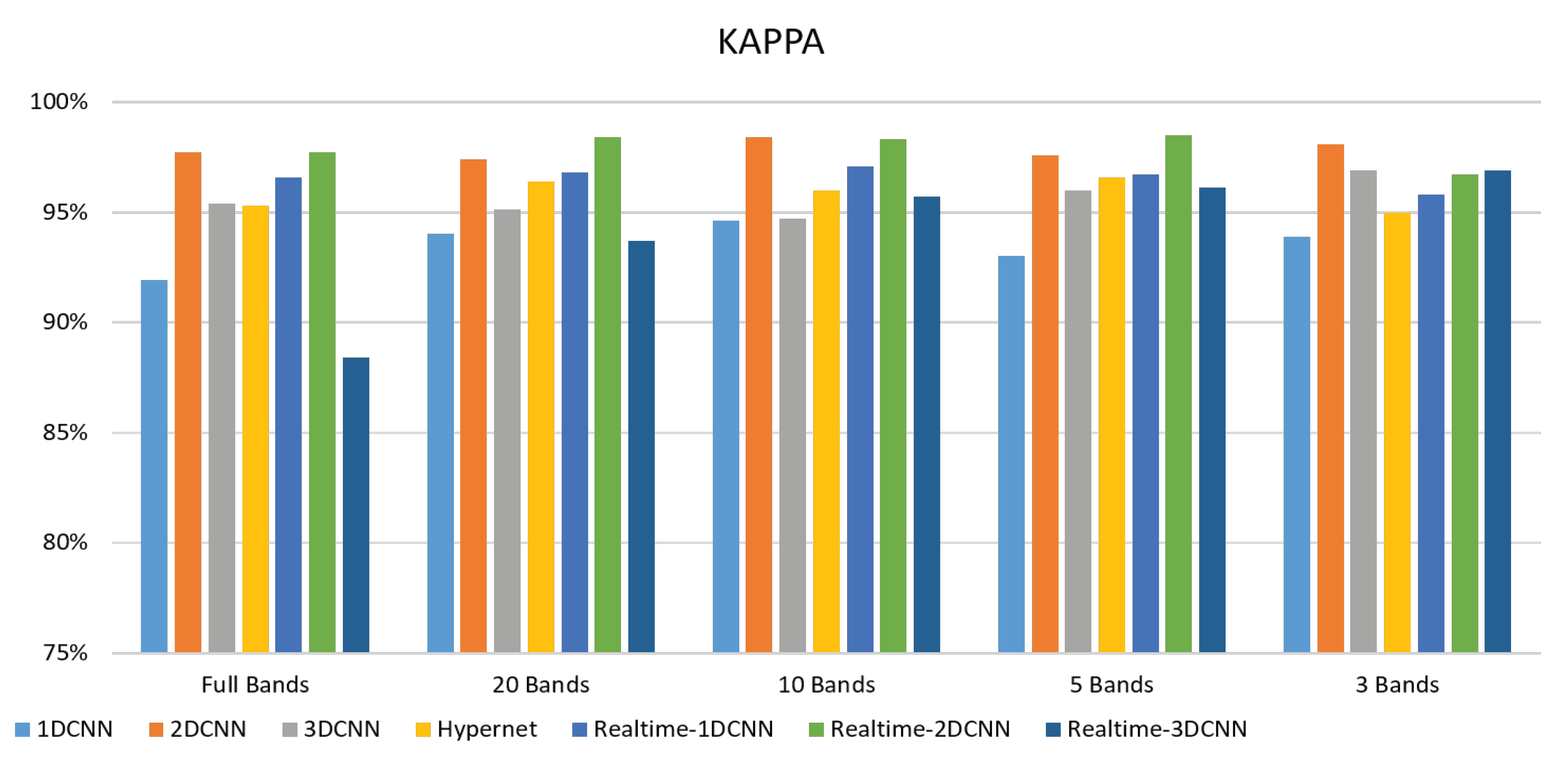
The snapshot camera uses filter discs for spectral sampling. The spectral information is relatively discrete. The FX10 push-broom camera performs spectral sampling by light splitting so the information is continuous and relatively complete. Therefore, if a network with a few layers is used, different features can be learned from the discrete signals. This avoids learning meaningless information or too much information with similar features. The real-time-1DCNN performs an average operation for the spatial information of the target object, losing spatial information and keeping spectral information that can be used for classification. Although the accuracy of real-time-1DCNN was higher than 95%, it was lower than that of the two models (realtime-2DCNN and realtime-3DCNN). A smaller number of bands leads to a faster speed. Therefore, real-time-1DCNN is unsuitable in practice. Realtime-2DCNN had the highest accuracy of 98% in this study, possibly because only spatial information was considered. The advantage of real-time-2DCNN is that the speed could be 40 (FPS). While this speed was not as fast as realtime-1DCNN, it was faster than realtime-3DCNN. The Realtime-2DCNN model with 5 bands had the most accurate model. The overall computing time was shortened a lot as the convolution was reduced. Realtime-2DCNN model had the steadiest accuracy among the three models. The real-time-3DCNN was not the most accurate model. This might be because the real-time-3DCNN considers the spatial and spectral information simultaneously. It could also be possible that there was only one convolution layer, and the important features could not be extracted.
Figure 31.
Snapshot camera hyperspectral ACC histogram.
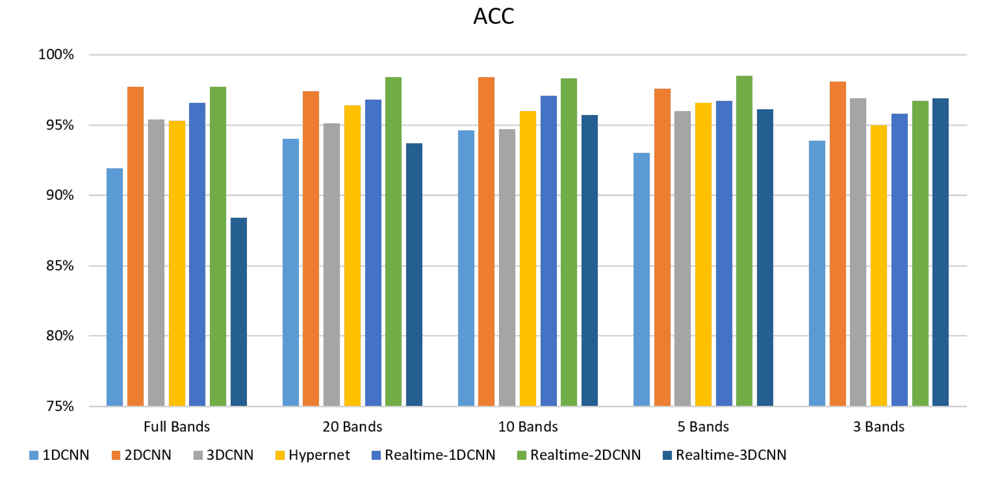
Figure 32.
Snapshot camera hyperspectral KAPPA histogram.
5. Conclusions
Currently, the classification of peanuts on the market is mostly based on visual identification. However, visual fatigue is likely to induce misrecognition when selecting large quantities. Color sorters are on the market, but their accuracy is only 70% or 80%. To solve this problem, the spectral analysis technique was required. The surface features were used, and the spectral information of targets was captured to fuse their spatial information. In this study, the FX10 push-broom camera was used for shooting, and 1,557 peanut shells were used for training, with 777 healthy and plump peanuts and 780 defective peanuts. Feasibility and high accuracy were determined first, then the snapshot camera was used for shooting and analyses. There were 2,700 peanut shells for training, with 1,350 healthy and plump peanuts and 1,350 defective peanuts. There were 4,257 peanut samples collected in this study, including normal, insect bite, underdevelopment, and rupture. First, the band selection was performed for the image. Then the samples were classified using 1D-CNN, 2D-CNN, 3D-CNN, real-time-1DCNN, realtime-2DCNN, and real-time-3DCNN. Finally, the FX10 push-broom camera was used for detection. The maximum accuracy was 98%, and Kappa was 97%. With the snapshot camera, the maximum detection accuracy was 98%, and Kappa was 97%. The training data were augmented by random rotation and horizontal and vertical flipping. This helped achieve steady model performance and accuracy. The contributions of this study are given below:
- (1)
- The FX10 had a lot of data/information. The ACC was 98% when the 3DCNN was used for analysis. On the contrary, the ACC of the snapshot was 98% when the 2DCNN was used. The number of convolution layers was reduced.
- (2)
- With the assistance of peanut farmers, more than 4,000 hyperspectral peanut images were collected. A database was created to get closer to the practical situation.
- (3)
- A 2DCNN model based on spatial information was developed. A good recognition rate could be achieved. The recognition speed could reach real-time, which was about 40 (FPS).
- (4)
- The PCA has been successfully used for selecting important and representative bands. The main characteristic bands were between 700 and 850 nm.
References
- Thenkabail, P. S., Smith, R. B., & De Pauw, E. (2000). Hyperspectral vegetation indices and their relationships with agricultural crop characteristics. Remote sensing of Environment, 71(2), 158-182.
- Dale, L. M., Thewis, A., Boudry, C., Rotar, I., Dardenne, P., Baeten, V., & Pierna, J. A. F. (2013). Hyperspectral imaging applications in agriculture and agro-food product quality and safety control: A review. Applied Spectroscopy Reviews, 48(2), 142-159.
- Adão, T., Hruška, J., Pádua, L., Bessa, J., Peres, E., Morais, R., & Sousa, J. J. (2017). Hyperspectral imaging: A review on UAV-based sensors, data processing and applications for agriculture and forestry. Remote Sensing, 9(11), 1110.
- Council of Agriculture, Executive Yuan. (2001). Peanut. https://www.coa.gov.tw/ws.php?id=1012&print=Y.
- Huang, L., He, H., Chen, W., Ren, X., Chen, Y., Zhou, X., Xia, Y., Wang, X., Jiang, X., & Liao, B. (2015). Quantitative trait locus analysis of agronomic and quality-related traits in cultivated peanut (Arachis hypogaea L.). Theoretical and Applied Genetics, 128(6), 1103-1115.
- Bindlish, E., Abbott, A. L., & Balota, M. (2017). Assessment of peanut pod maturity. 2017 IEEE Winter Conference on Applications of Computer Vision (WACV).
- Jiang, J., Qiao, X., & He, R. (2016). Use of Near-Infrared hyperspectral images to identify moldy peanuts. Journal of Food Engineering, 169, 284-290.
- Qi, X., Jiang, J., Cui, X., & Yuan, D. (2019). Identification of fungi-contaminated peanuts using hyperspectral imaging technology and joint sparse representation model. Journal of food science and technology, 56(7), 3195-3204.
- Han, Z., & Gao, J. (2019). Pixel-level aflatoxin detecting based on deep learning and hyperspectral imaging. Computers and Electronics in Agriculture, 164, 104888.
- Xueming He, Chen Yan, Xuesong Jiang, Fei Shen, Jie You, Yong Fang (2021) Classification of aflatoxin B1 naturally contaminated peanut using visible and near-infrared hyperspectral imaging by integrating spectral and texture features.
- Liu, Z., Jiang, J., Qiao, X., Qi, X., Pan, Y., & Pan, X. (2020). Using convolution neural network and hyperspectral image to identify moldy peanut kernels. LWT, 132, 109815.
- Zou, S., Tseng, Y.-C., Zare, A., Rowland, D. L., Tillman, B. L., & Yoon, S.-C. (2019). Peanut maturity classification using hyperspectral imagery. biosystems engineering, 188, 165-177.
- Qi, H., Liang, Y., Ding, Q., & Zou, J. (2021). Automatic Identification of Peanut-Leaf Diseases Based on Stack Ensemble. Applied Sciences, 11(4), 1950.
- Dunteman, G. H. (1989). Principal components analysis. Sage.
- Martinez, A. M., & Kak, A. C. (2001). Pca versus lda. IEEE transactions on pattern analysis and machine intelligence, 23(2), 228-233.
- Chang, C.-I., Du, Q., Sun, T.-L., & Althouse, M. L. (1999). A joint band prioritization and band-decorrelation approach to band selection for hyperspectral image classification. IEEE Transactions on Geoscience and Remote Sensing, 37(6), 2631-2641.
- Al-Amri, S. S., & Kalyankar, N. V. (2010). Image segmentation by using threshold techniques. arXiv preprint arXiv:1005.4020.
- Wu, K., Otoo, E., & Shoshani, A. (2005). Optimizing connected component labeling algorithms. Medical Imaging 2005: Image Processing,.
- Suzuki, S. (1985). Topological structural analysis of digitized binary images by border following. Computer vision, graphics, and image processing, 30(1), 32-46.
- Wang, Ping, et al. “Deep Convolutional Neural Network for Coffee Bean Inspection.” Sensors and Materials 33.7 (2021): 2299-2310.
- Murphy, R. J., Monteiro, S. T., & Schneider, S. (2012). Evaluating classification techniques for mapping vertical geology using field-based hyperspectral sensors. IEEE Transactions on Geoscience and Remote Sensing, 50(8), 3066-3080.
- Singh, C. B., Jayas, D. S., Paliwal, J. N. D. G., & White, N. D. G. (2009). Detection of insect-damaged wheat kernels using near-infrared hyperspectral imaging. Journal of stored products research, 45(3), 151-158.
- Qin, J., Burks, T. F., Ritenour, M. A., & Bonn, W. G. (2009). Detection of citrus canker using hyperspectral reflectance imaging with spectral information divergence. Journal of food engineering, 93(2), 183-191.
- Hestir, E. L., Brando, V. E., Bresciani, M., Giardino, C., Matta, E., Villa, P., & Dekker, A. G. (2015). Measuring freshwater aquatic ecosystems: The need for a hyperspectral global mapping satellite mission. Remote Sensing of Environment, 167, 181-195.
- Chen, S. Y., Lin, C., Tai, C. H., & Chuang, S. J. (2018). Adaptive window-based constrained energy minimization for detection of newly grown tree leaves. Remote Sensing, 10(1), 96.
- Chen S-Y, Lin C, Chuang S-J, Kao Z-Y. Weighted Background Suppression Target Detection Using Sparse Image Enhancement Technique for Newly Grown Tree Leaves. Remote Sensing. 2019; 11(9):1081.
- Tiwari, K. C., Arora, M. K., & Singh, D. (2011). An assessment of independent component analysis for detection of military targets from hyperspectral images. International Journal of Applied Earth Observation and Geoinformation, 13(5), 730-740.
- Chen, S. Y., Cheng, Y. C., Yang, W. L., & Wang, M. Y. (2021). Surface defect detection of wet-blue leather using hyperspectral imaging. IEEE Access, 9, 127685-127702.
- Kelley, D. B., Goyal, A. K., Zhu, N., Wood, D. A., Myers, T. R., Kotidis, P & Müller, A. (2017, May). High-speed mid-infrared hyperspectral imaging using quantum cascade lasers. In Chemical, Biological, Radiological, Nuclear, and Explosives (CBRNE) Sensing XVIII (Vol. 10183, p. 1018304). International Society for Optics and Photonics.
- Dai, Q., Cheng, J. H., Sun, D. W., & Zeng, X. A. (2015). Advances in feature selection methods for hyperspectral image processing in food industry applications: A review. Critical reviews in food science and nutrition, 55(10), 1368-1382.
- Ariana, D. P., Lu, R., & Guyer, D. E. (2006). Near-infrared hyperspectral reflectance imaging for detection of bruises on pickling cucumbers. Computers and electronics in agriculture, 53(1), 60-70.
- Li, D., Zhang, J., Zhang, Q., & Wei, X. (2017, October). Classification of ECG signals based on 1D convolution neural network. In 2017 IEEE 19th International Conference on e-Health Networking, Applications and Services (Healthcom) (pp. 1-6). IEEE.
- Hsieh, T.-H., & Kiang, J.-F. (2020). Comparison of CNN algorithms on hyperspectral image classification in agricultural lands. Sensors, 20(6), 1734.
- Pang, L., Men, S., Yan, L., & Xiao, J. (2020). Rapid vitality estimation and prediction of corn seeds based on spectra and images using deep learning and hyperspectral imaging techniques. IEEE Access, 8, 123026-123036.
- Yang, D., Hou, N., Lu, J., & Ji, D. (2022). Novel leakage detection by ensemble 1DCNN-VAPSO-SVM in oil and gas pipeline systems. Applied Soft Computing, 115, 108212.
- Laban, N., Abdellatif, B., Moushier, H., & Tolba, M. (2021). Enhanced pixel based urban area classification of satellite images using convolutional neural network. International Journal of Intelligent Computing and Information Sciences, 21(3), 13-28.
- Wang, C., Liu, B., Liu, L., Zhu, Y., Hou, J., Liu, P., & Li, X. (2021). A review of deep learning used in the hyperspectral image analysis for agriculture. Artificial Intelligence Review, 1-49.
- M Rustowicz, R., Cheong, R., Wang, L., Ermon, S., Burke, M., & Lobell, D. (2019). Semantic segmentation of crop type in Africa: A novel dataset and analysis of deep learning methods. Proceedings of the IEEE/CVF Conference on Computer Vision and Pattern Recognition Workshops,.
- Moreno-Revelo, M. Y., Guachi-Guachi, L., Gómez-Mendoza, J. B., Revelo-Fuelagán, J., & Peluffo-Ordóñez, D. H. (2021). Enhanced Convolutional-Neural-Network Architecture for Crop Classification. Applied Sciences, 11(9), 4292.
- Toraman, S. (2020). Preictal and Interictal Recognition for Epileptic Seizure Prediction Using Pre-trained 2DCNN Models. Traitement du Signal, 37(6).
- Ji, S., Xu, W., Yang, M., & Yu, K. (2012). 3D convolutional neural networks for human action recognition. IEEE transactions on pattern analysis and machine intelligence, 35(1), 221-231.
- Saveliev, A., Uzdiaev, M., & Dmitrii, M. (2019). Aggressive action recognition using 3d cnn architectures. 2019 12th International Conference on Developments in eSystems Engineering (DeSE).
- Ji, S., Zhang, C., Xu, A., Shi, Y., & Duan, Y. (2018). 3D convolutional neural networks for crop classification with multi-temporal remote sensing images. Remote Sensing, 10(1), 75.
- Ji, S., Zhang, Z., Zhang, C., Wei, S., Lu, M., & Duan, Y. (2020). Learning discriminative spatiotemporal features for precise crop classification from multi-temporal satellite images. International Journal of Remote Sensing, 41(8), 3162-3174.
Figure 1.
Peanut classification procedure.
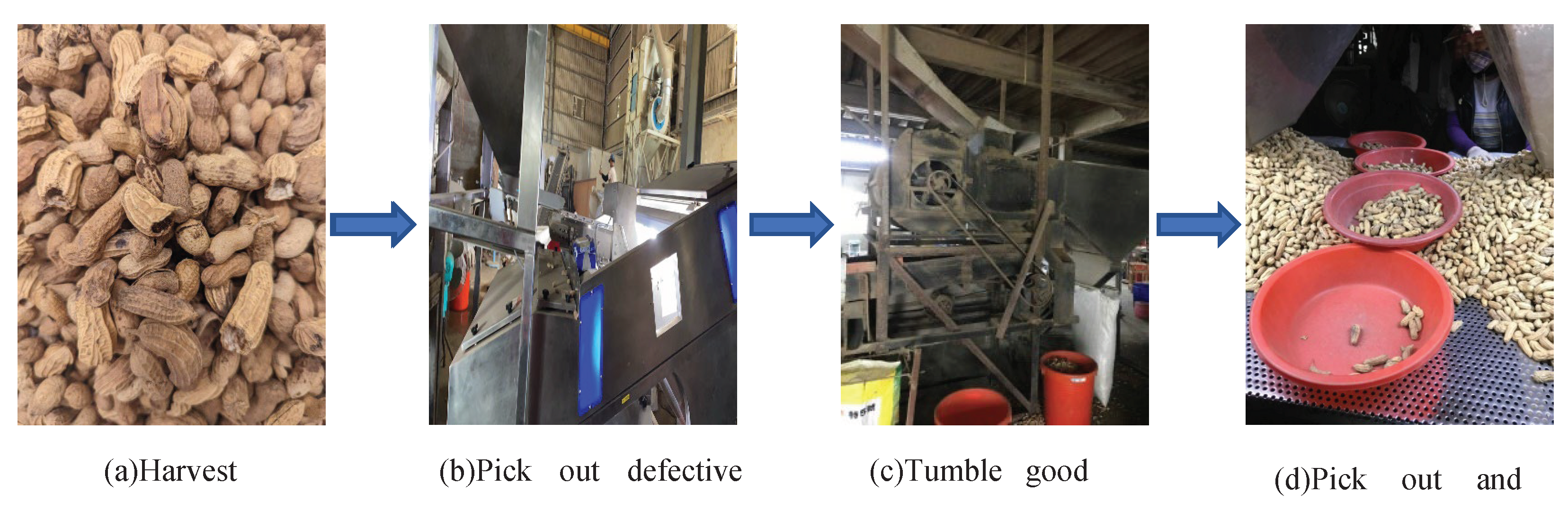
Figure 2.
The appearances of normal and defective peanuts (a) a healthy peanut, (b) underdevelopment, (c) insect bite, (d) a ruptured peanut (with kernels), (e) a ruptured peanut (without kernels).
Figure 2.
The appearances of normal and defective peanuts (a) a healthy peanut, (b) underdevelopment, (c) insect bite, (d) a ruptured peanut (with kernels), (e) a ruptured peanut (without kernels).
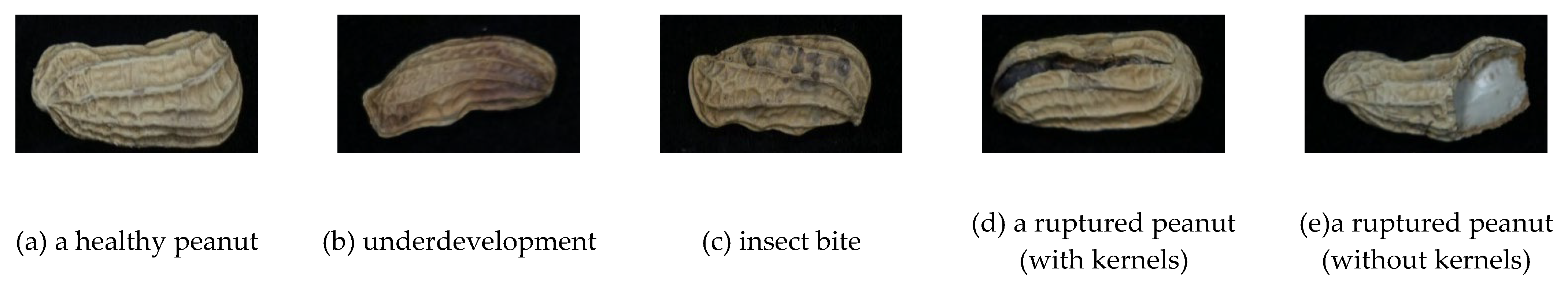
Figure 3.
Hyperspectral imaging system (a) FX10 hyperspectral camera, (b) snapshot hyperspectral camera.
Figure 3.
Hyperspectral imaging system (a) FX10 hyperspectral camera, (b) snapshot hyperspectral camera.
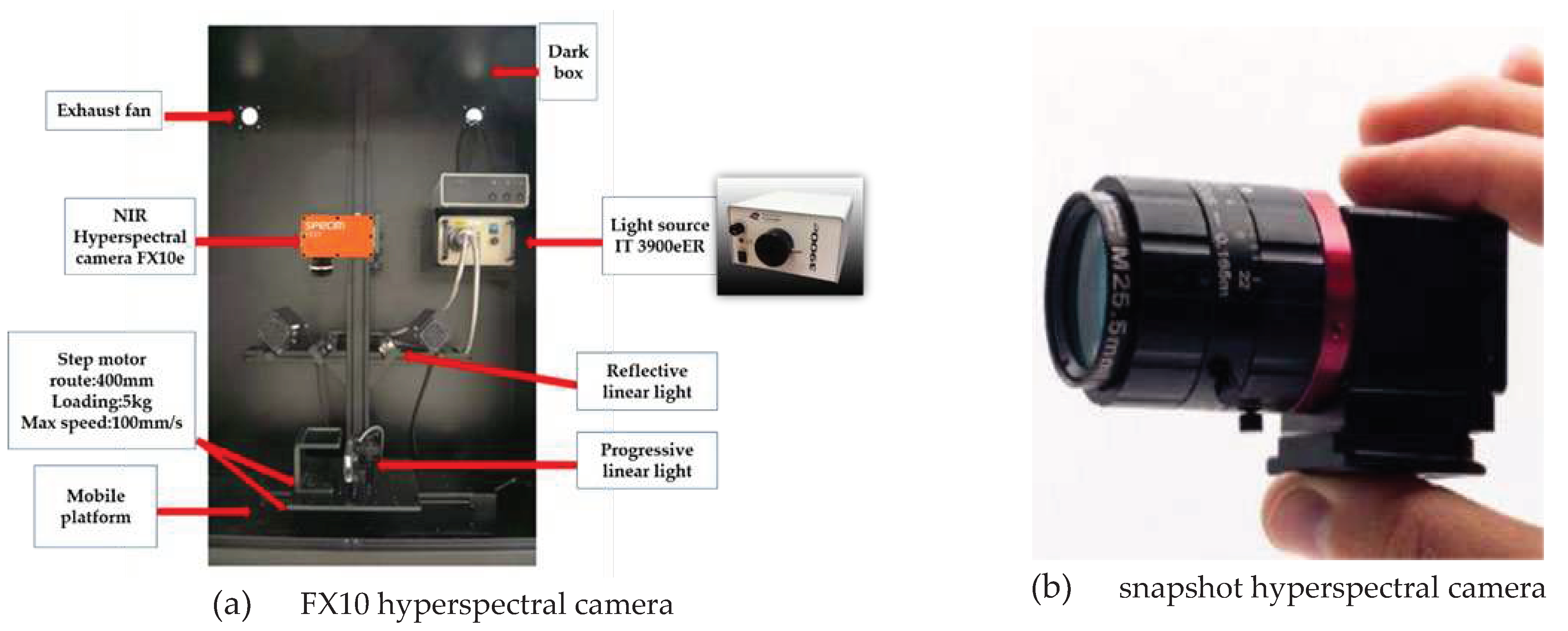
Figure 4.
Peanut color image (RGB) (a) FX10 hyperspectral camera, (b) snapshot hyperspectral camera.
Figure 4.
Peanut color image (RGB) (a) FX10 hyperspectral camera, (b) snapshot hyperspectral camera.
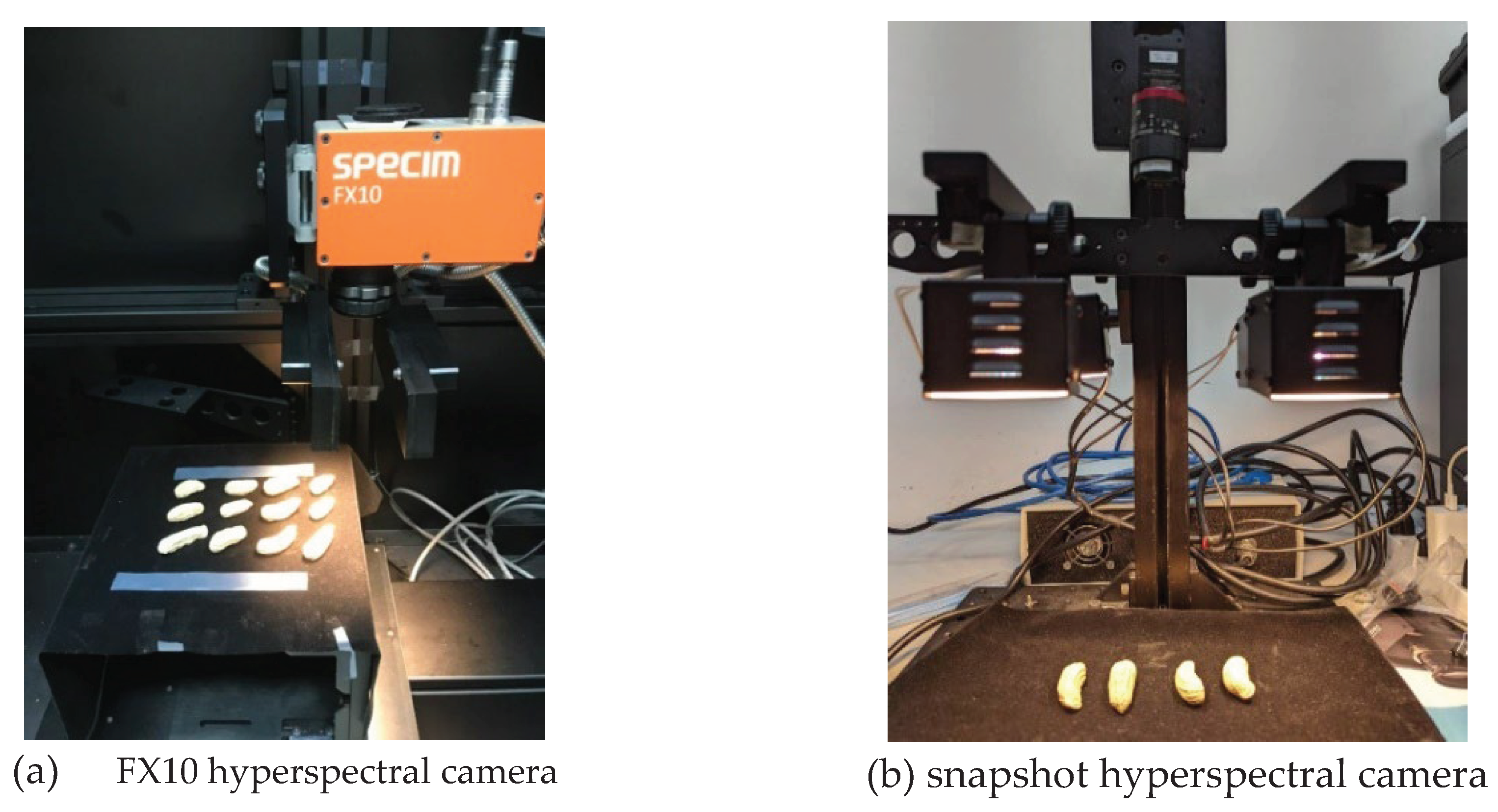
Figure 5.
Spectrum signals of normal and defective peanuts (a) spectrum signals of different states of FX10 hyperspectral cameras (b) spectrum signals of different states of Snapshot hyperspectral camera.
Figure 5.
Spectrum signals of normal and defective peanuts (a) spectrum signals of different states of FX10 hyperspectral cameras (b) spectrum signals of different states of Snapshot hyperspectral camera.
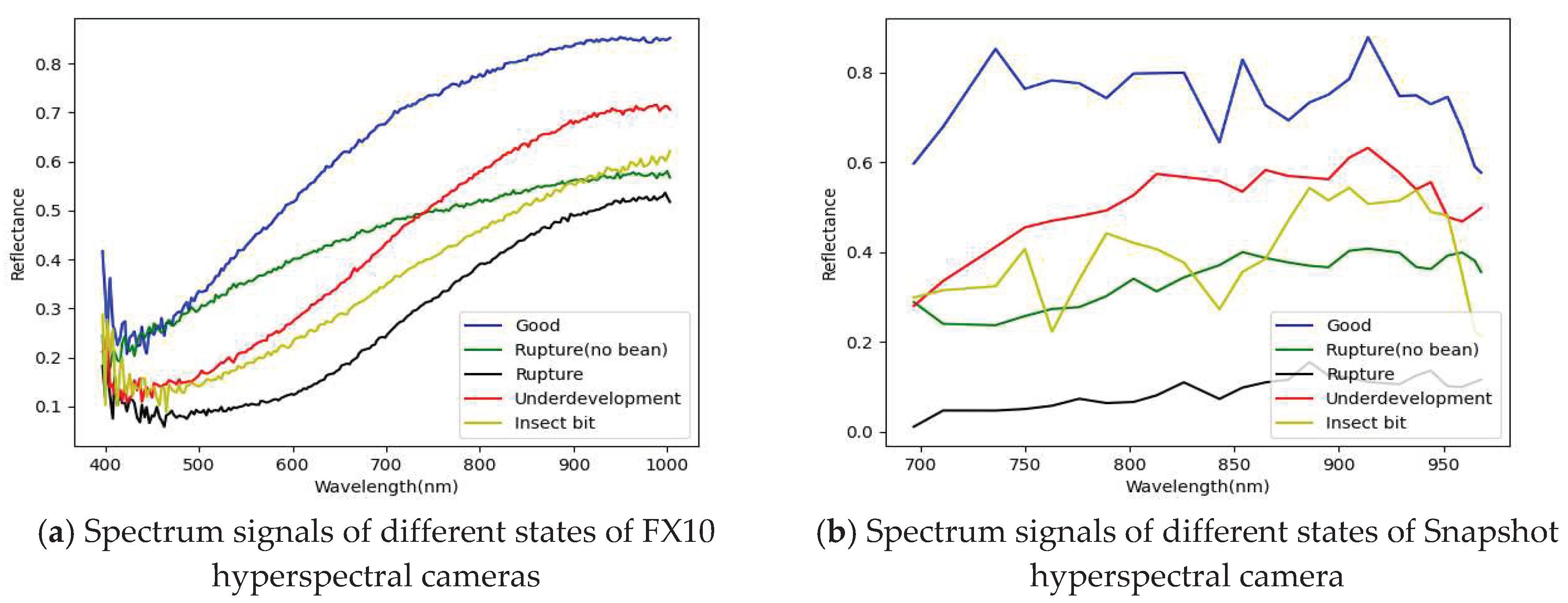
Figure 6.
A plot of the PCA projection vectors.
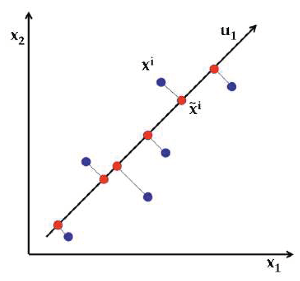
Figure 7.
ROI peanut images.
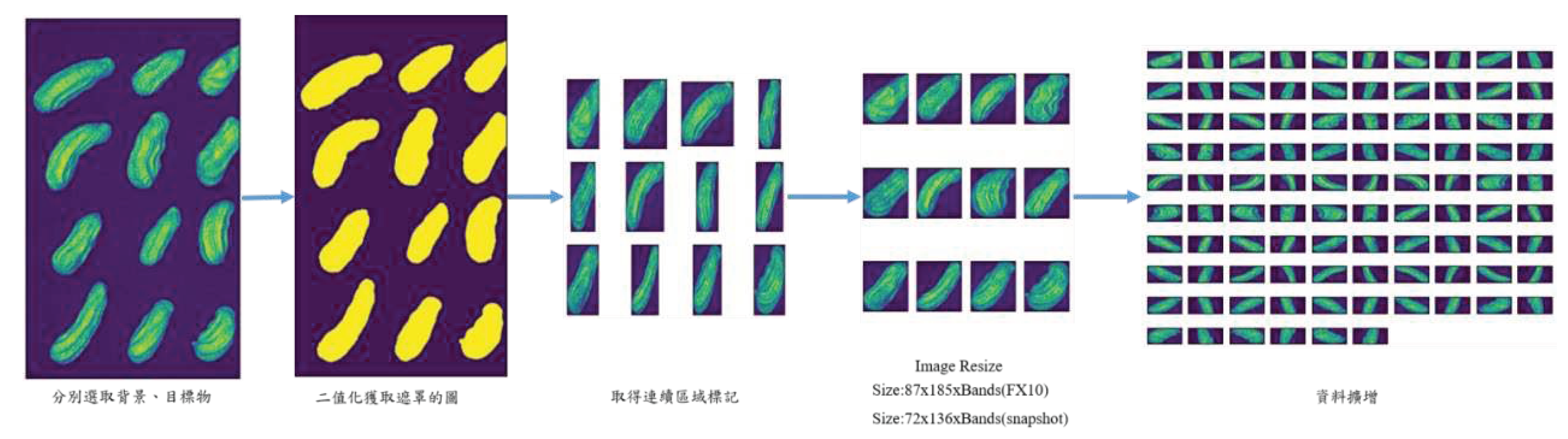
Figure 8.
1D-CNN model.
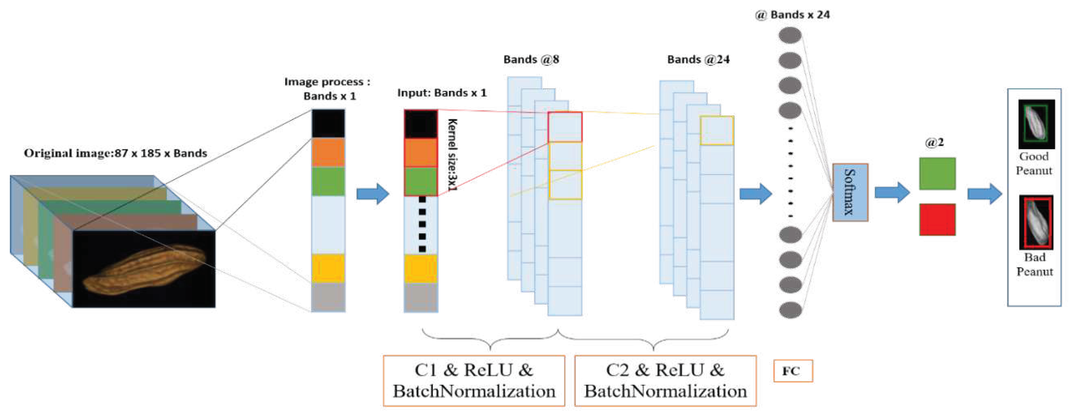
Figure 10.
1D-CNN model.
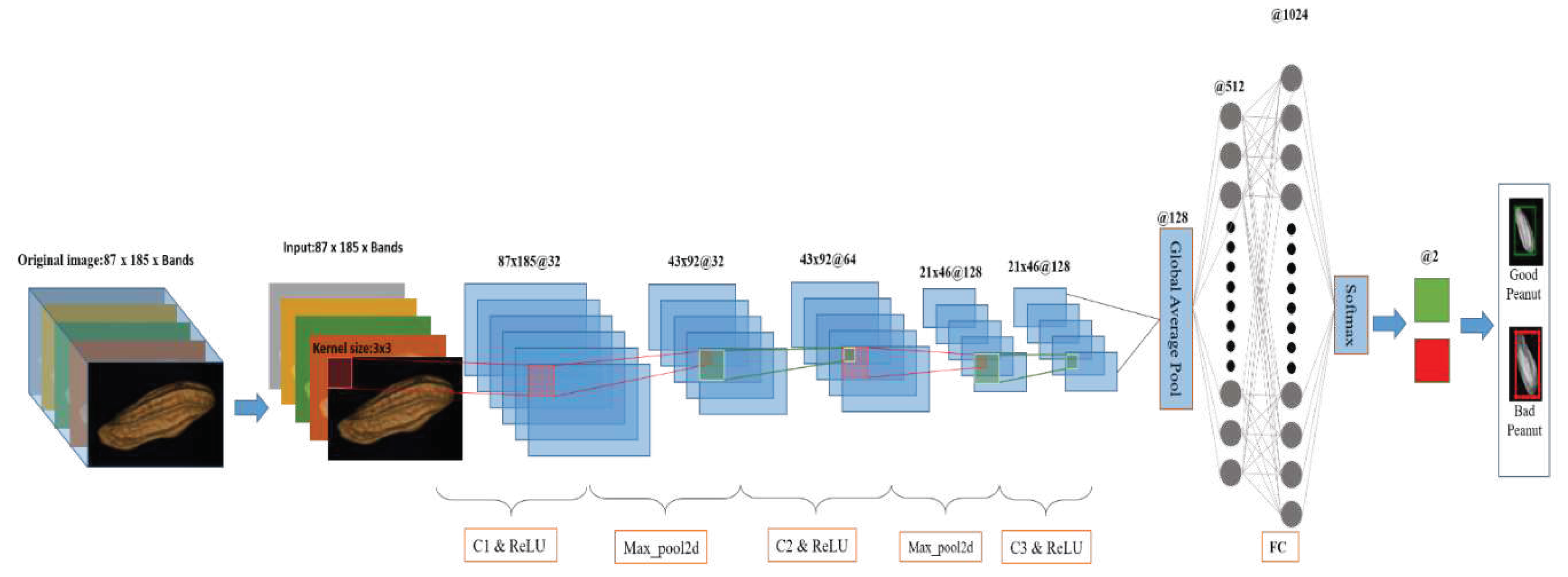
Figure 11.
Realtime-2DCNN model.
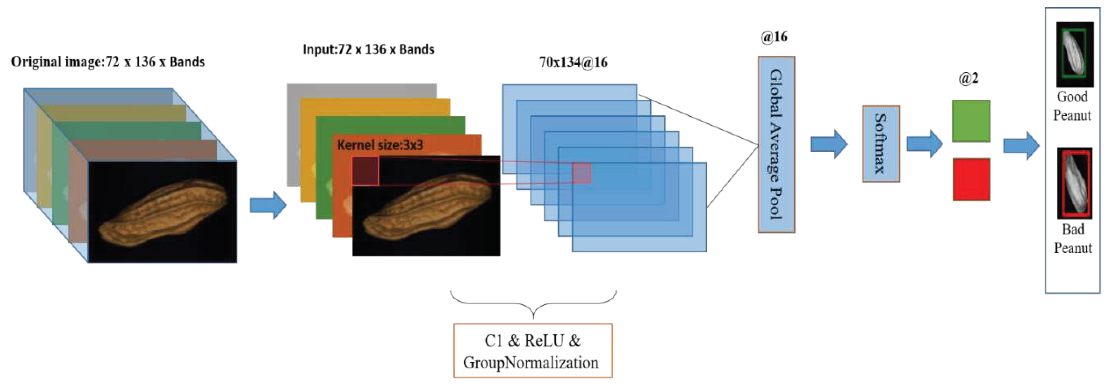
Figure 12.
3D-CNN Model.
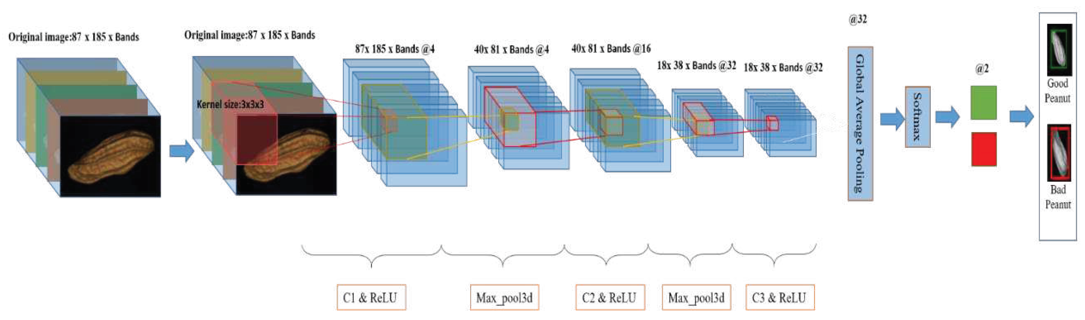
Figure 13.
Realtime-3DCNN model.

Figure 14.
Flow chart.
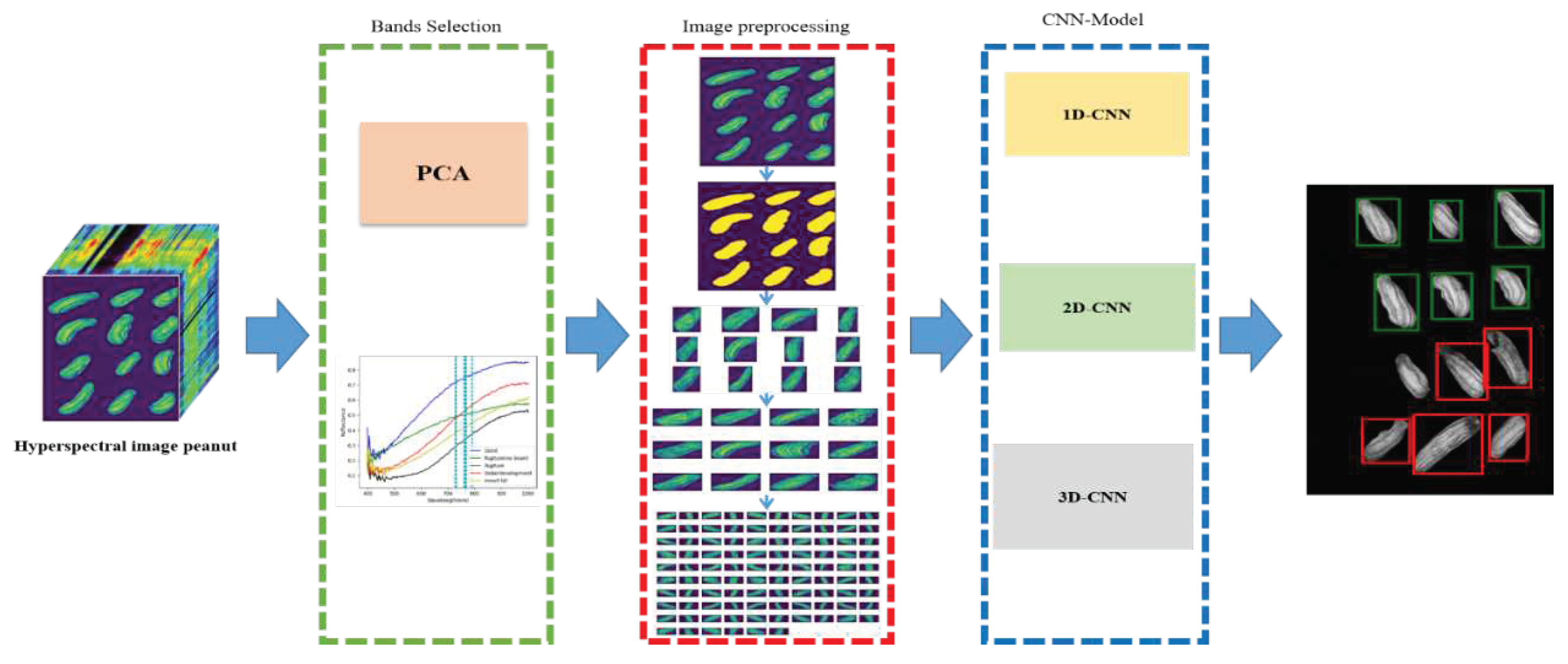
Figure 15.
Visualization after PCA band selection (a) 20 Bands selection results, (b) 10 Bands selection results, (c) 5 Bands selection results, (d) 3 Bands selection results.
Figure 15.
Visualization after PCA band selection (a) 20 Bands selection results, (b) 10 Bands selection results, (c) 5 Bands selection results, (d) 3 Bands selection results.
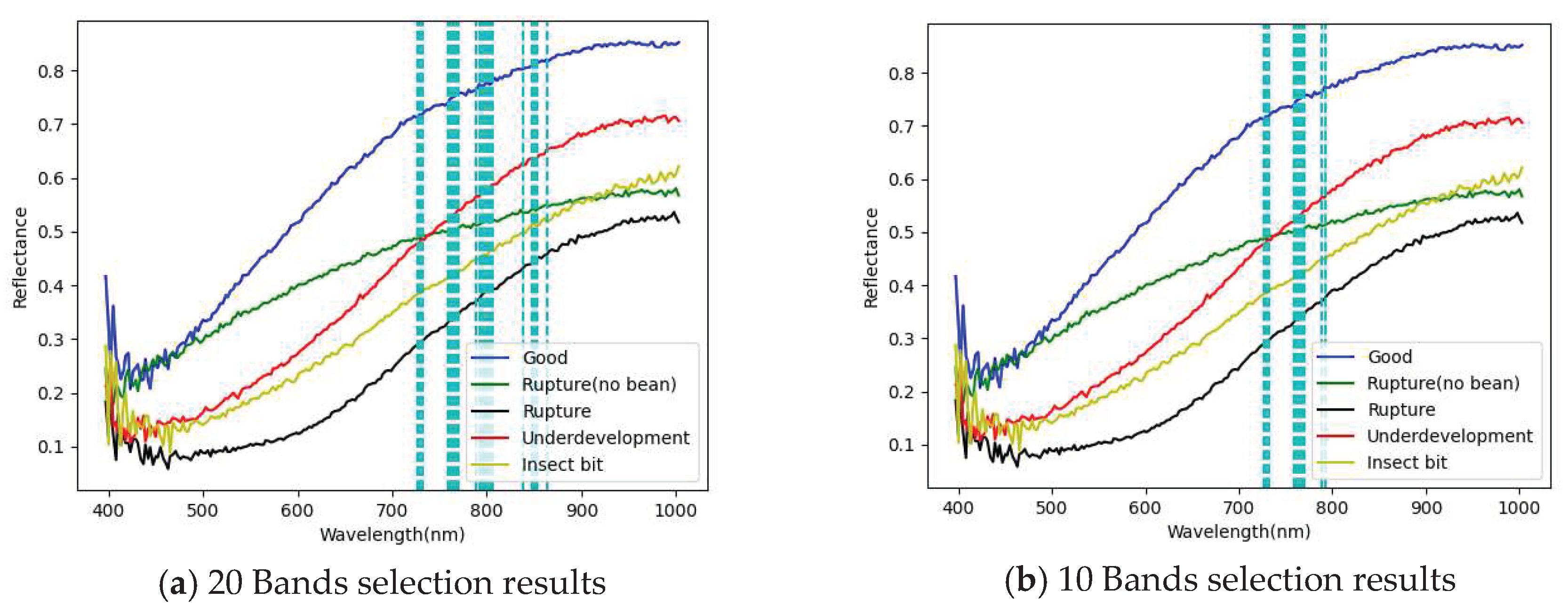
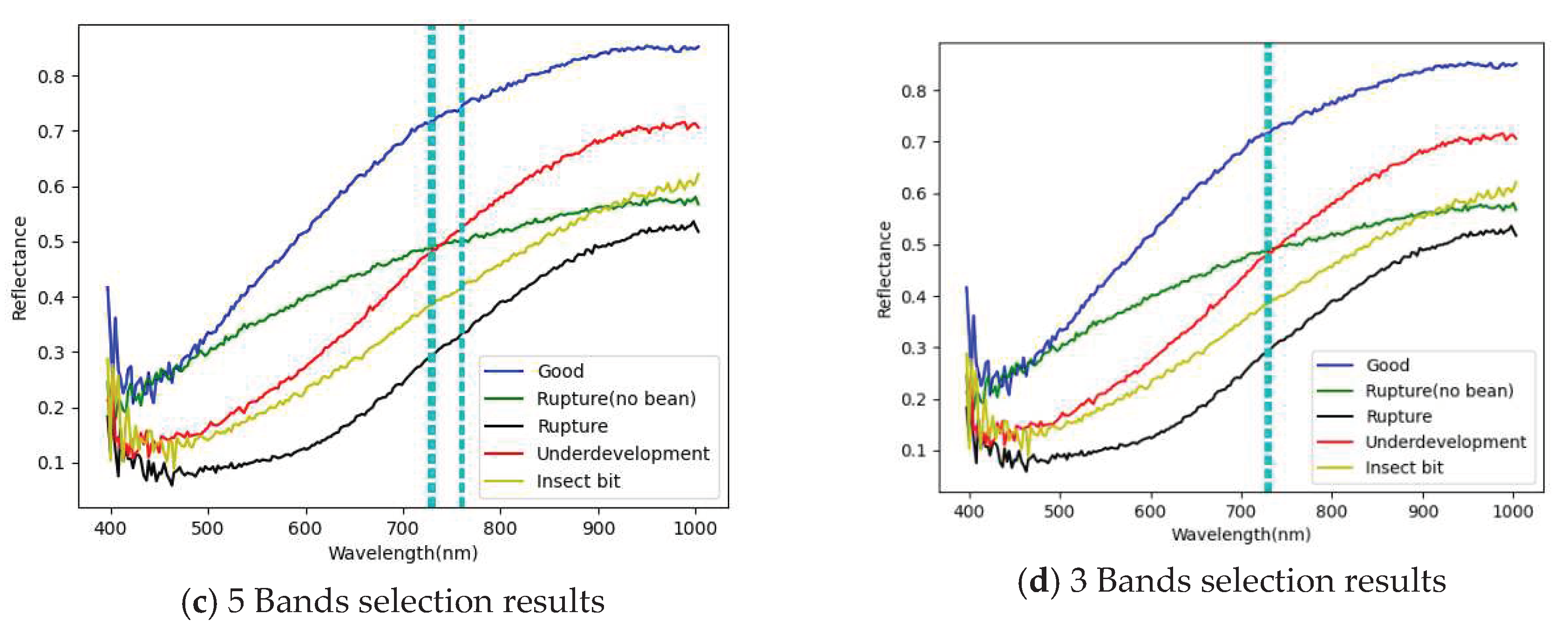
Figure 16.
PCA band selection result visualization (a) 20 Bands selection results, (b) 10 Bands selection results, (c) 5 Bands selection results, (d) 3 Bands selection results.
Figure 16.
PCA band selection result visualization (a) 20 Bands selection results, (b) 10 Bands selection results, (c) 5 Bands selection results, (d) 3 Bands selection results.
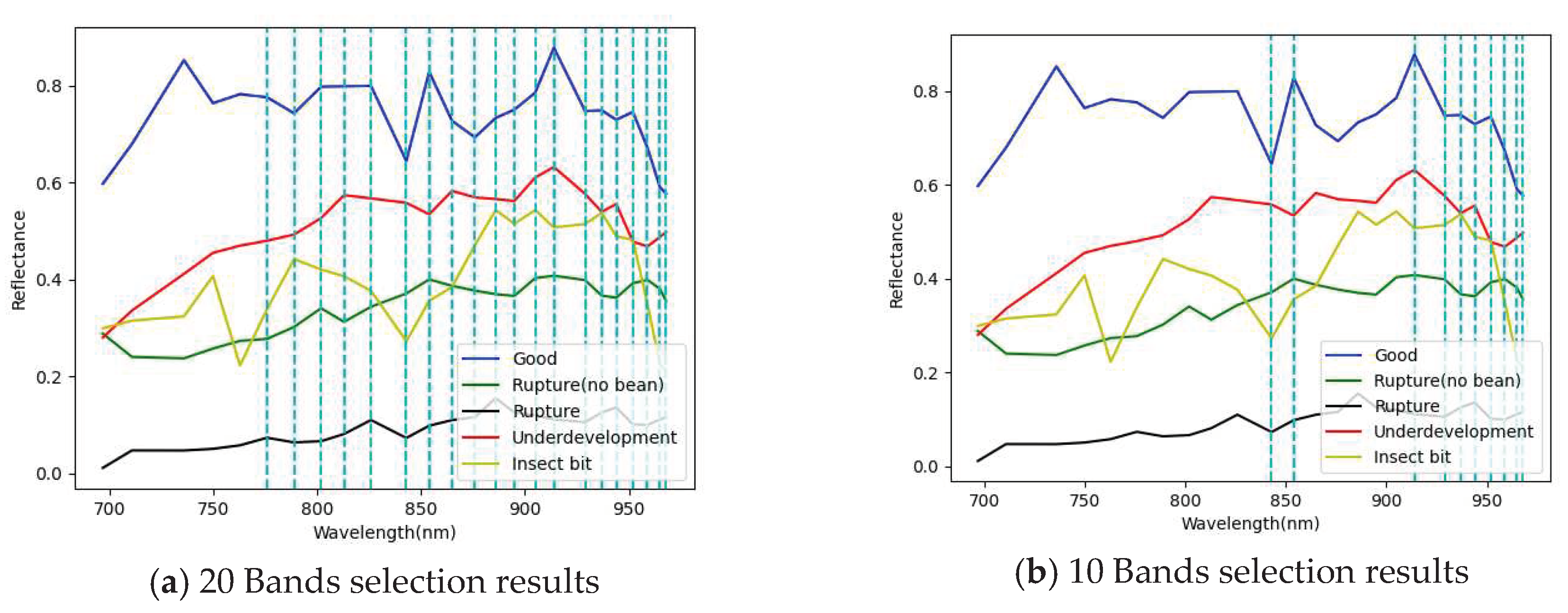
Figure 23.
RGB peanut original image.
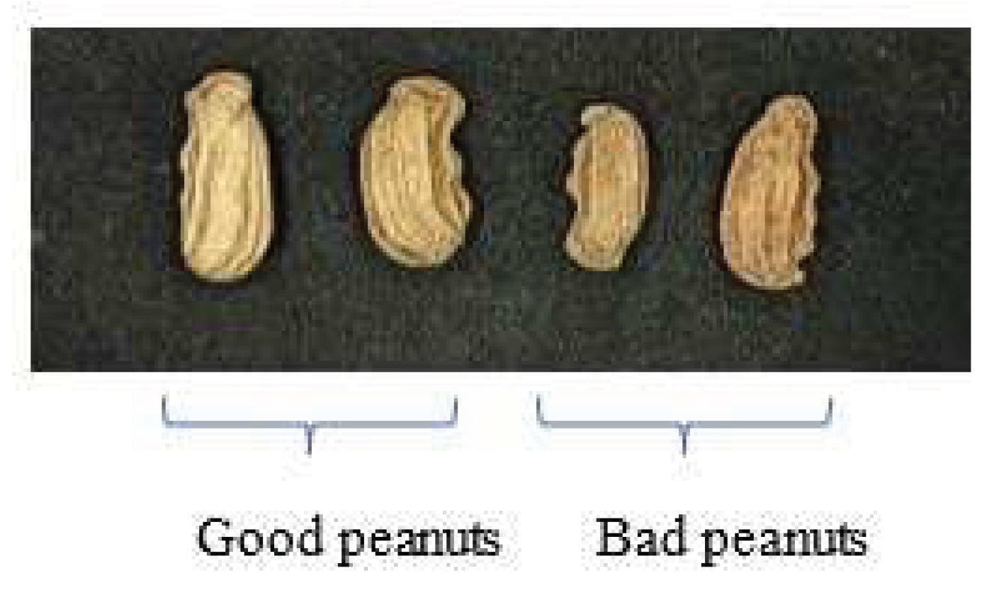
Figure 24.
All band results of peanuts. Green represents healthy peanuts, Red represents defective peanuts, and the unframed peanuts represent misrecognition.
Figure 24.
All band results of peanuts. Green represents healthy peanuts, Red represents defective peanuts, and the unframed peanuts represent misrecognition.
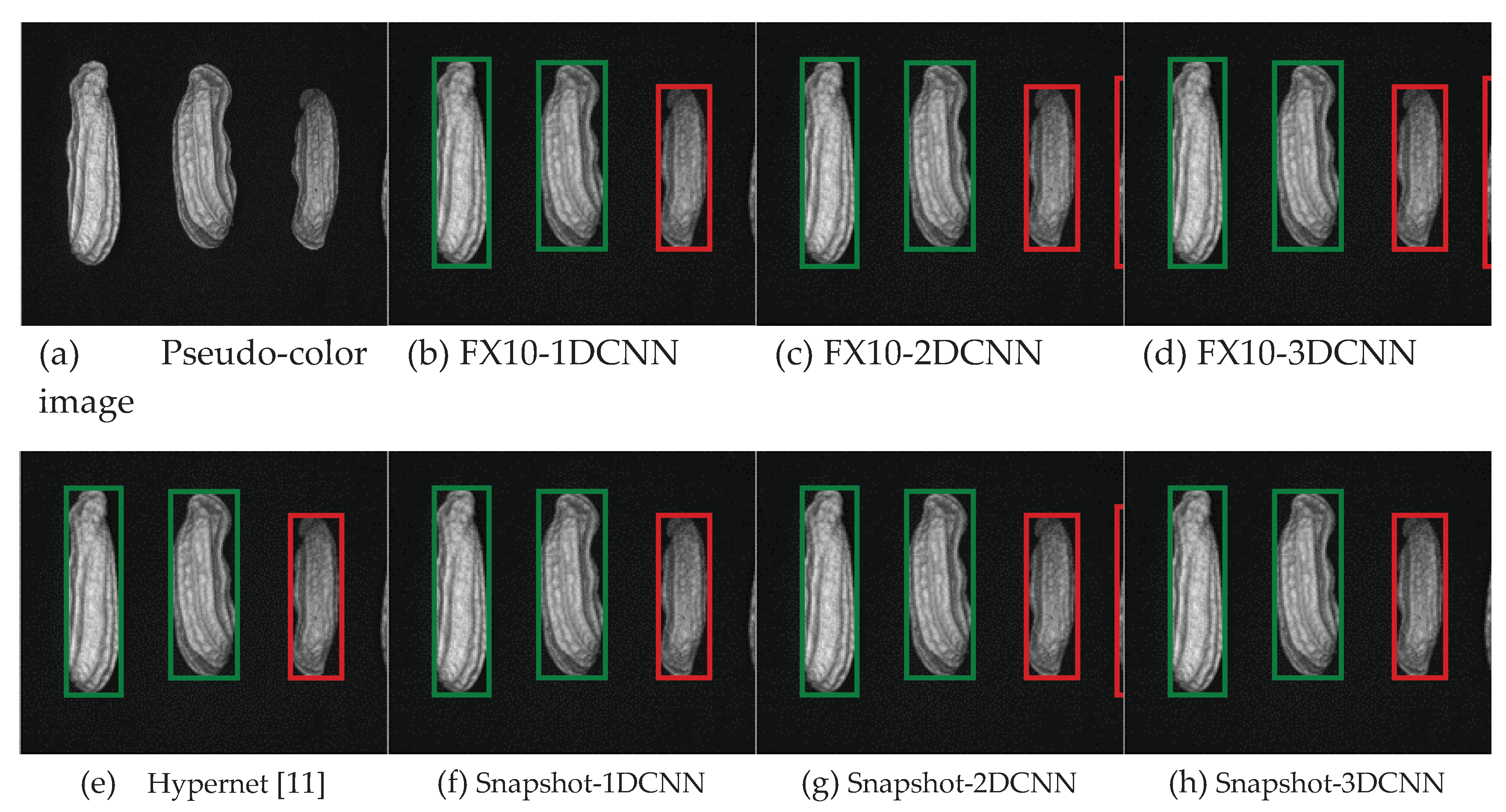
Figure 25.
Classification results of 20 bands. Green represents healthy peanuts, Red represents defective peanuts, and the unframed peanuts represent misrecognition.
Figure 25.
Classification results of 20 bands. Green represents healthy peanuts, Red represents defective peanuts, and the unframed peanuts represent misrecognition.
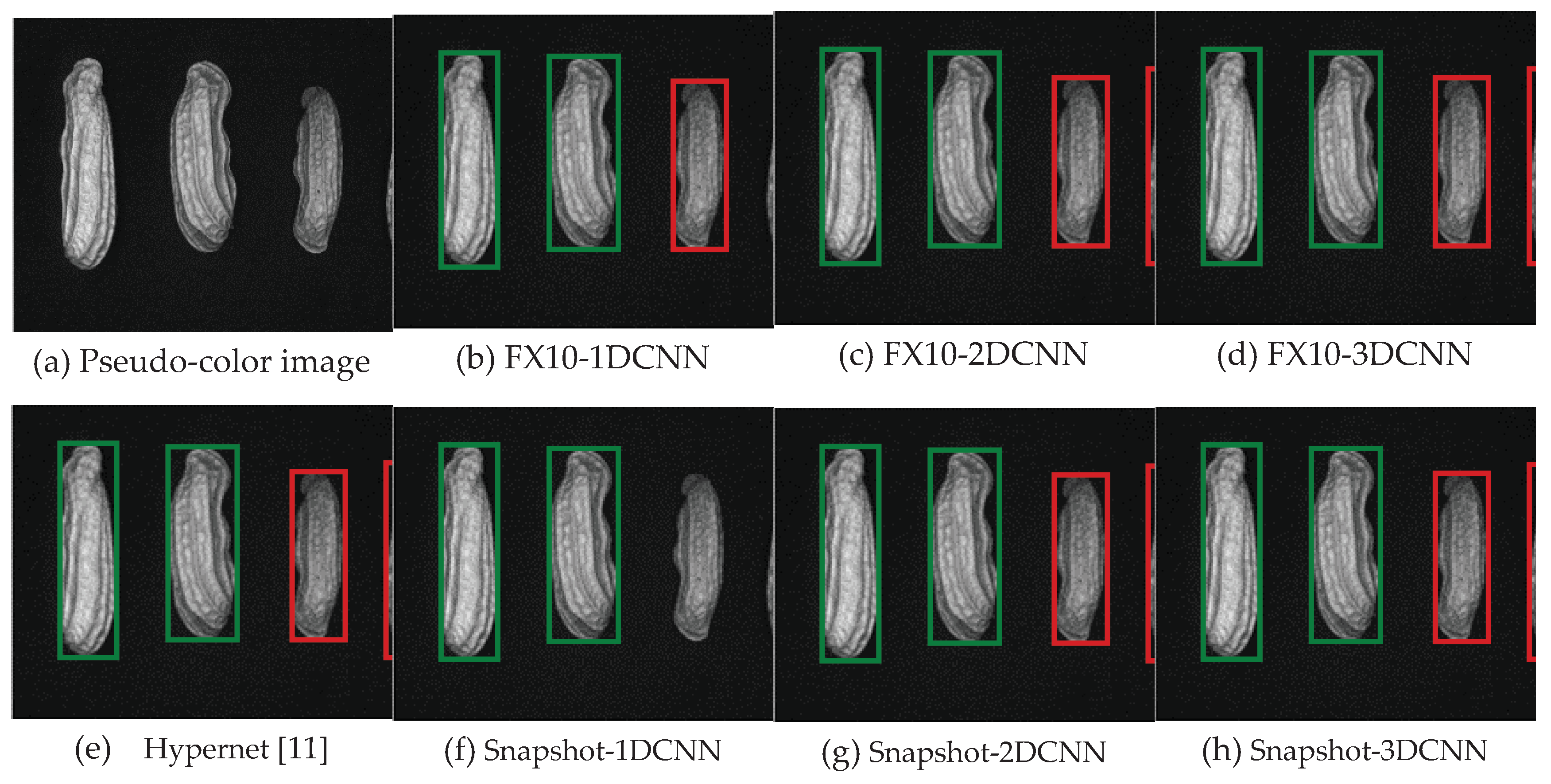
Figure 26.
Classification results of 10 bands. Green represents healthy peanuts, Red represents defective peanuts, and the unframed peanuts represent misrecognition.
Figure 26.
Classification results of 10 bands. Green represents healthy peanuts, Red represents defective peanuts, and the unframed peanuts represent misrecognition.
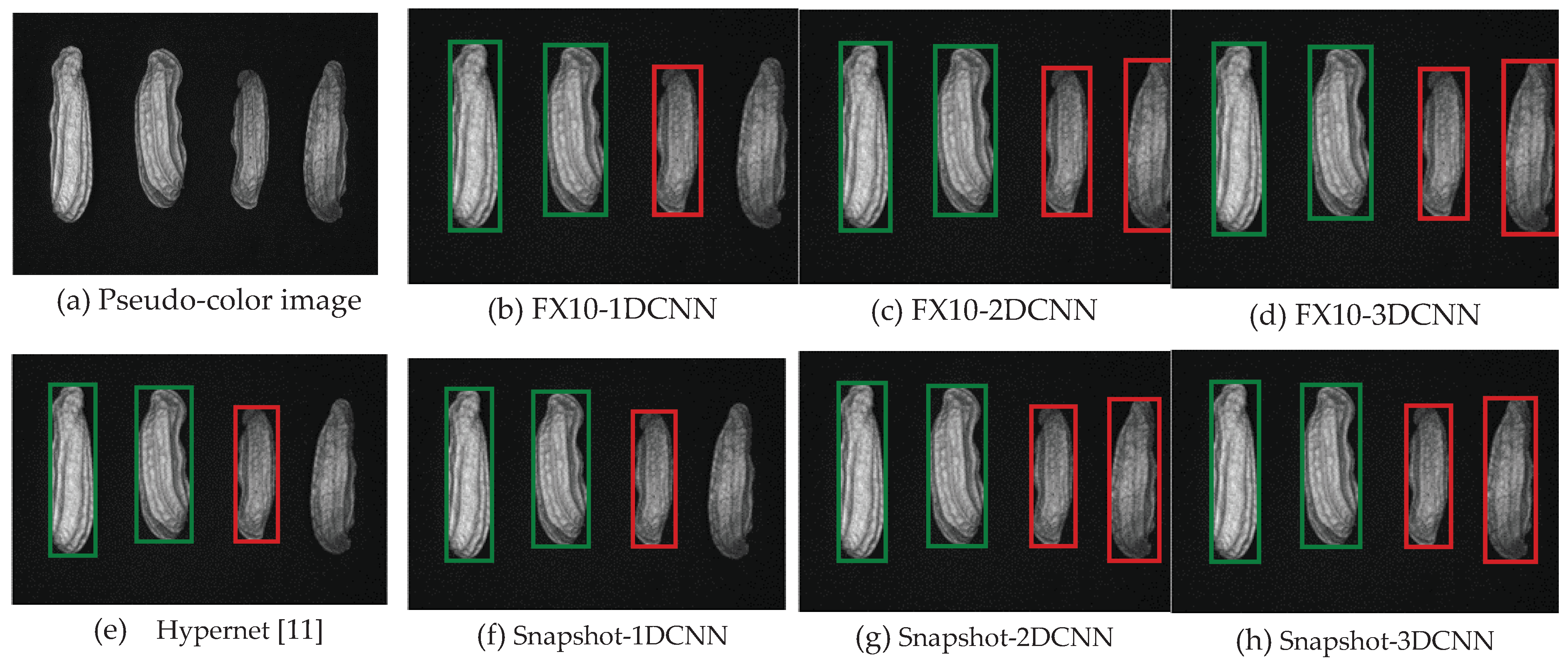
Figure 27.
Classification results of 10 bands. Green represents healthy peanuts, Red represents defective peanuts, and the unframed peanuts represent misrecognition.
Figure 27.
Classification results of 10 bands. Green represents healthy peanuts, Red represents defective peanuts, and the unframed peanuts represent misrecognition.
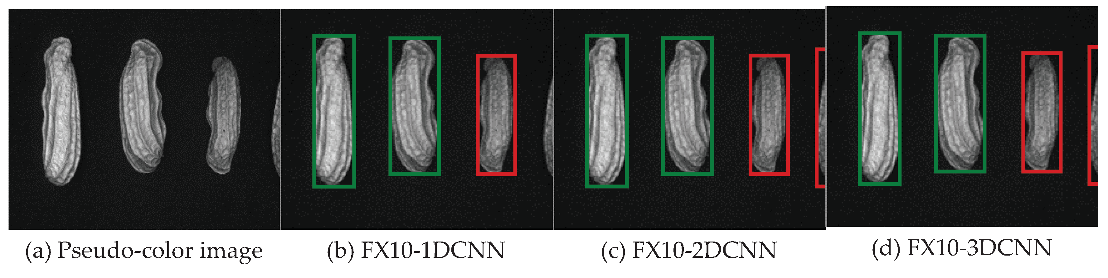
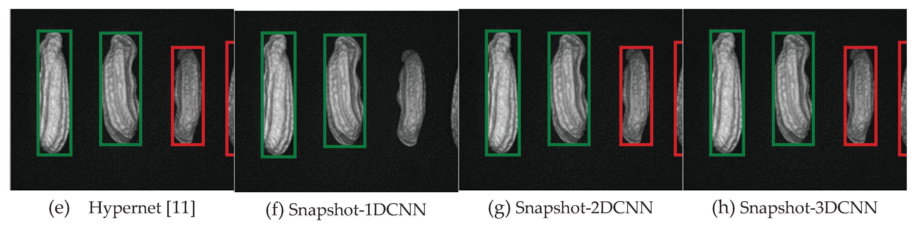
Figure 28.
Classification results of 3 bands. Green represents healthy peanuts, Red represents defective peanuts, and the unframed peanuts represent misrecognition.
Figure 28.
Classification results of 3 bands. Green represents healthy peanuts, Red represents defective peanuts, and the unframed peanuts represent misrecognition.
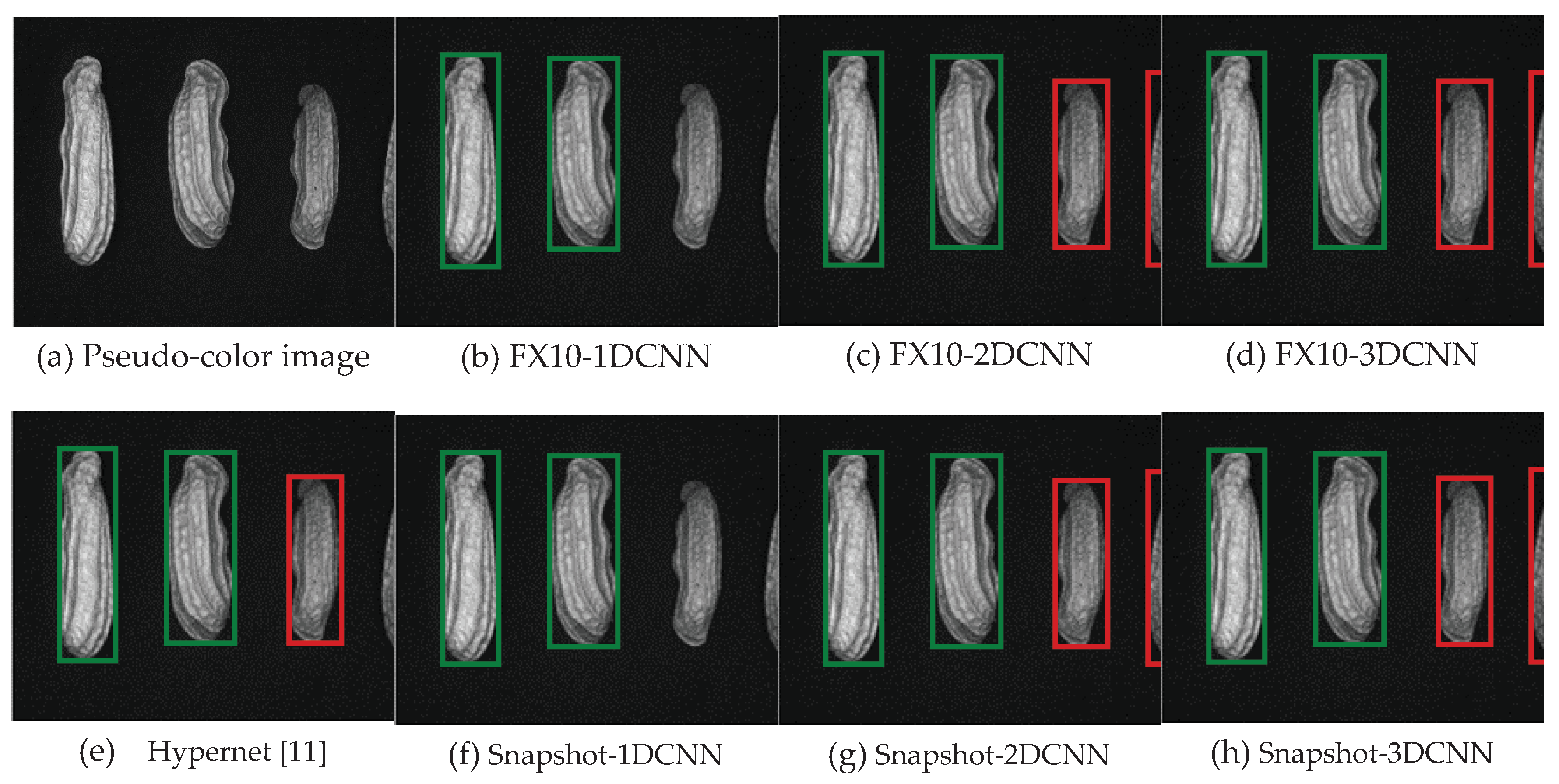

Table 1.
Comparison of documents about peanut defect detection.
| References | Detection target | Spectral range (nm) | Data quantity | Data analysis | Overall accuracy |
|---|---|---|---|---|---|
| (Jiang et al., 2016) [7] | Aflatoxin | 970-2,570 nm | 149 pcs | PCA+ Threshold | 98.7 |
| (Qi et al., 2019) [8] | Aflatoxin | 967-2,499 nm | 2,312 pixels | JSRC+SVM | 98.4 |
| (Han & Gao, 2019) [9] | Aflatoxin | 292-865 nm | 146 pcs | CNN | 96 |
| (Zou et al., 2019) [12] | Peanut shell maturity | 400-1,000 nm | 540 pcs | LMM+RGB | 91.15 |
| (Liu et al., 2020) [11] | Aflatoxin | 400-1000 nm | 1,066 pcs | Unet, Hypernet | 92.07 |
| (Qi et al., 2021) [13] | Peanut leaves | RGB | 3,205 images | GoogleNet | 97.59 |
| (Xueming et al., 2021) [10] | Aflatoxin | 400-1,000 nm | 150 pcs | SGS+SNV | 94 |
Table 2.
Sample quantity for FX10 experiment.
| Classification | Normal Peanut | Defect Peanut | Total |
|---|---|---|---|
| Training amount | 237 | 240 | 477 |
| Testing amount | 540 | 540 | 1080 |
| Total | 777 | 780 | 1557 |
Table 3.
Sample quantity for Snapshot experiment.
| Classification | Normal Peanut | Defect Peanut | Total |
|---|---|---|---|
| Training amount | 350 | 350 | 700 |
| Testing amount | 1000 | 1000 | 2000 |
| Total | 1350 | 1350 | 2700 |
Table 4.
band selection.
| Analysis method | Important band |
|---|---|
| PCA 20 Band | 726.33,729.06,731.79,759.14,761.88,764.62,767.36,770.11, 789.33,792.08,794.84,797.59,800.34,803.1, 805.85,838.98,847.29,852.83, 850.06, 863.92 |
| PCA 10 Band | 726,729,731,759,761,764,767,770,789,792, |
| PCA 5 Band | 726,729,731,759,761 |
| PCA 3 Band | 726,729,731 |
Table 5.
band selection.
| Analysis method | Important band |
|---|---|
| 20 Band | 854, 843, 929, 914, 959, 968, 965, 952, 944, 937, 905, 895, 886, 876, 865, 826, 813, 802, 789, 776 |
| 10 Band | 854, 843, 929, 914, 959, 968, 965, 952, 944, 937 |
| 5 Band | 854, 843, 929, 914, 959 |
| 3 Band | 854, 843, 929 |
Table 6.
Comparison table of bands selected from hyperspectral data captured by FX10 camera with different models.
Table 6.
Comparison table of bands selected from hyperspectral data captured by FX10 camera with different models.
| Model | Number of bands | TPR | FPR | Acc | Kappa | Runtime(ms) |
|---|---|---|---|---|---|---|
| 1D-CNN | Full band | 0.92 | 0.29 | 0.83 | 0.67 | 44.2 |
| 20 bands | 0.937 | 0.002 | 0.967 | 0.935 | 35.4 | |
| 10 bands | 0.924 | 0.024 | 0.962 | 0.908 | 32.8 | |
| 5 bands | 0.913 | 0.023 | 0.956 | 0.907 | 31.1 | |
| 3 bands | 0.91 | 0.03 | 0.954 | 0.904 | 30.7 | |
| 2D-CNN | Full band | 0.94 | 0.07 | 0.971 | 0.940 | 58 |
| 20 bands | 0.959 | 0.004 | 0.977 | 0.956 | 32.6 | |
| 10 bands | 0.956 | 0.062 | 0.977 | 0.933 | 28.6 | |
| 5 bands | 0.957 | 0.011 | 0.973 | 0.941 | 26.9 | |
| 3 bands | 0.94 | 0.07 | 0.96 | 0.93 | 26 | |
| 3D-CNN | Full band | 0.990 | 0.170 | 0.910 | 0.820 | 61 |
| 20 bands | 0.980 | 0.013 | 0.983 | 0.967 | 37 | |
| 10 bands | 0.967 | 0.035 | 0.981 | 0.961 | 32.8 | |
| 5 bands | 0.961 | 0.068 | 0.978 | 0.957 | 30.5 | |
| 3 bands | 1.0 | 0.05 | 0.97 | 0.94 | 29.3 | |
| Hypernet [11] | Full band | 0.14 | 0.93 | 0.85 | 54.5 | |
| 20 bands | 0.964 | 0.0736 | 0.9444 | 0.888 | 32.3 | |
| 10 bands | 0.9634 | 0.1020 | 0.9277 | 0.855 | 29.6 | |
| 5 bands | 0.98787 | 0.07692 | 0.9527 | 0.90546 | 25.7 | |
| 3 bands | 0.9875 | 0.1 | 0.938 | 0.87 | 25.4 | |
| Realtime-1DCNN | Full band | 0.92307 | 0.1764 | 0.86666 | 0.73333 | 51.2 |
| 20 bands | 1.0 | 0.150 | 0.9111 | 0.82222 | 23.4 | |
| 10 bands | 0.98 | 0.07 | 0.96 | 0.922 | 23.2 | |
| 5 bands | 0.976 | 0.077 | 0.958 | 0.91 | 23 | |
| 3 bands | 0.8823 | 0.09 | 0.9333 | 0.866666 | 22.8 | |
| Realtime-2DCNN | Full band | 0.96 | 0.1 | 0.94 | 0.85 | 51.8 |
| 20 bands | 0.98 | 0.04 | 0.93 | 0.87 | 31.4 | |
| 10 bands | 0.98 | 0.07 | 0.9505 | 0.90 | 28 | |
| 5 bands | 0.961 | 0.068 | 0.978 | 0.957 | 26 | |
| 3 bands | 1 | 0.06 | 0.96 | 0.92 | 25.2 | |
| Realtime-3DCNN | Full band | 0.99 | 0.17 | 0.91 | 0.82 | 72.1 |
| 20 bands | 0.99 | 0.05 | 0.966 | 0.933 | 34.4 | |
| 10 bands | 0.99 | 0.05 | 0.966 | 0.933 | 32.3 | |
| 5 bands | 0.961 | 0.068 | 0.978 | 0.957 | 29.3 | |
| 3 bands | 1 | 0.07 | 0.95 | 0.91 | 24.4 |
Disclaimer/Publisher’s Note: The statements, opinions and data contained in all publications are solely those of the individual author(s) and contributor(s) and not of MDPI and/or the editor(s). MDPI and/or the editor(s) disclaim responsibility for any injury to people or property resulting from any ideas, methods, instructions or products referred to in the content. |
© 2023 by the authors. Licensee MDPI, Basel, Switzerland. This article is an open access article distributed under the terms and conditions of the Creative Commons Attribution (CC BY) license (http://creativecommons.org/licenses/by/4.0/).
Copyright: This open access article is published under a Creative Commons CC BY 4.0 license, which permit the free download, distribution, and reuse, provided that the author and preprint are cited in any reuse.


