
Submitted:
29 May 2023
Posted:
30 May 2023
You are already at the latest version
Abstract
In the present paper we introduce three new classes of bi-univalent functions connected with Gregory coefficients. For functions in each of these three bi-univalent function classes we have derived the estimates of the Taylor--Maclaurin coefficients $\left|a_{2}\right|$ and $\left|a_{3}\right|$ and Fekete-Szeg\H{o} functional problems for functions belonging to these new subclasses. We defined three subclasses of the class of the bi-univalent functions $\Sigma$, namely $\mathfrak{HG}_{\Sigma}$, $\mathfrak{GM}_{\Sigma}(\mu)$ and $\mathfrak{G}_{\Sigma}(\lambda)$ by using the subordinations with the function whose coefficients are Gregory's numbers. First, we proved that these classes are not empty, i.e. contains other functions than the identity one. Using the well-known Carath\'eodory Lemma for the functions with real positive parts in the open unit disk, together with an estimation due to P. Zaprawa (see https://doi.org/10.1155/2014/357480) and another one of Libera and Zlotkiewicz, we gave upper bounds for the above mentioned initial coefficients and for the Fekete-Szeg\H{o} functionals. The main results are followed by some particular cases, and the novelty of the definitions and the proofs could involve further studies for such type of similarly defined subclasses.
Keywords:
univalent functions
; bi-univalent functions
; starlike and convex functions of some order
; subordination
; Fekete-Szeg\H{o} problem
MSC: 30C45; 30C50; 30C80
1. Definitions and preliminaries
Let denote the class of all analytic functions f defined in the open unit disk and normalized by the conditions and . Thus, each has a Taylor–Maclaurin series expansion of the form
Further, let denote the class of all functions which are univalent in .
Let the functions f and g be analytic in . We say that the function f is subordinate to g, written as , if there exists a function , which is analytic in with
such that
Besides, if the function g is univalent in , then the following equivalence holds:
It is well known that every function has an inverse , defined by
and
Suppose that has an analytic continuation to . Then, the function f is said to be bi-univalent in if both f and are univalent in . In this case let
and let denote the class of bi-univalent functions in given by (1). Examples of functions in the class are, for example
However, the familiar Koebe function is not a member of , while other common examples of analytic functions in such
are also not members of . Lewin [1] investigated the bi-univalent function class and showed that . Subsequently, Brannan and Clunie [2] conjectured that . Netanyahu [3], on the other hand, showed that . The coefficient estimate problem for each of the Taylor–Maclaurin coefficients for , , is presumably still an open problem.
Similar to the familiar subclasses and of starlike and convex function of order , , respectively, Brannan and Taha [4] (see also [5]) introduced certain subclasses of the bi-univalent function class , namely the subclasses and of bi-starlike functions and of bi-convex functions of order , , respectively. For each of the function classes and they found non-sharp estimates of the first two Taylor–Maclaurin coefficients and . In fact, Srivastava et al. [6] have actually revived the study of analytic and bi-univalent functions in recent years for some intriguing examples of functions and characterization of the class (see [6,7,8,9,10,11,12,13,14]).
The Fekete-Szegő functional for is well known for its rich history in the field of Geometric Function Theory. Its origin was in the disproof by Fekete and Szegő [15] conjecture of Littlewood and Paley, that the coefficients of odd univalent functions are bounded by unity. This functional has since received great attention, particularly for many subclasses of the family of univalent functions. The problem of finding the sharp bounds for this functional of any compact family of functions for any complex is commonly known as the classical Fekete-Szegő problem (or inequality).
Gregory coefficients . Gregory coefficients also known as reciprocal logarithmic numbers, Bernoulli numbers of the second kind, or Cauchy numbers of the first kind, are the decrease rational numbers . They occur in the Maclaurin series expansion of the reciprocal logarithm
These numbers are named after James Gregory who introduced them in 1670 in the numerical integration context. They were subsequently rediscovered by many mathematicians and often appear in works of modern authors, Laplace, Mascheroni, Fontana, Bessel, Clausen, Hermit, Pearson and Fisher.
In this paper we considered the generating function of the Gregory coefficients (see [16,17]) to be given by
where the function log is considered at the main branch, that is . Clearly, for some values of are
Finding the upper bound for the Taylor coefficients have been one of the vital topic of research in Geometric function theory as it offers numerous properties for many subclasses of As. Therefore, we will be inquisitive about the subsequent hassle in this segment: find if for subclasses of univalent functions. In particular, bound for the second one coefficient offers growth and distortion theorems for features of those subclasses. Further, the use of the Hankel determinants (which also deals with the bounds of the coefficients), and we mention that Cantor [18] proved that “if ratio of two bounded analytic features in , then the function is rational”.
2. Coefficient bounds of the class
In 2010 Srivastava et al. [6] have actually revived the study of analytic and bi-univalent functions. Inspired by that, in this section we consider the class of analytic bi-univalent function relating with generating function of the Gregory coefficients to obtain initial coefficients and .
Definition 1.
are satisfied, and the function is defined by (2).
Remark 1.
1. For the function we have , , and using the 3D plot of the MAPLE™ computer software, we obtain that the image of the open unit disk by the function
is positive, hence is a starlike (and also univalent) function with respect to the point 1 (see Figure 1).
2. We would like to emphasize that the class is not empty. Thus, if we consider , , then it is easy to check that , and moreover, with .
Using the fact that for all it follows that . For the particular case , using the2D plotof the MAPLE™ computer software we obtain the image of the boundary by the functions , and shown in the Figure 2. Since is univalent in , the previous reason yields that the subordinations and hold whenever and (see Figure 2). Concluding, , hence the class is not empty and contains other functions than the identity.
In our first results we obtain the upper bounds for the modules of the first two coefficients for the functions that belong to the class given in Definition 1. Further, we use the following lemmas, which were introduced by Zaprawa in [19,20] and we will discuss the Fekete-Szegő functional problems [15].
Let , with , denotes the class of analytic functions p in with and , . Especially, we will use the notation instead of for the usual Carathéodory’s class of functions.
The next two lemmas will be used in our studies.
Lemma 1.
[21] If has the form , , then
and this inequality is sharp for each .
We mention that this inequality is the well-known result for the Carathéodory Lemma [21] (see also [22, Corollary 2.3, p. 41], 23, Carathéodory’s Lemma, p. 41]).
The second lemma is a generalization of Lemma 6 from [20] that could be obtained for :
Lemma 2.
[20, Lemma 7, p. 2] Let and . If and , then
The next result gives the upper bounds for the first two coefficients of the functions that belong to .
Theorem 1.
If is given by (1), then
Proof.
If , from the Definition 1 the subordinations (3) and (4) hold. Then, there exists an analytic function u in with and , , such that
and an analytic function v in with and , , such that
Therefore, the function
belongs to the class , hence
and
Similarly, the function
belongs to the class , therefore
and
Since the function g has the form (2), upon comparing the corresponding coefficients in (10) and (11) we get
If we add the equalities (13) and (15) we get
and substituting the value of from (17) in the right hand side of (18) we deduce that
Using (5) together with the triangle’s inequality in the relations (12) and (19) it follows
that proves our first result.
This relation combined with (12) leads to
Using the above values for and we will prove the following Fekete–Szegő type inequality for the functions of the class .
Theorem 2.
If is given by (1), then for any the next inequality holds:
3. Coefficient bounds for the class
In the second results we will obtain the upper bounds for the modules of the first two coefficients for the functions that belong to the class defined below, then we will study the Fekete-Szegő functional problems for this functions class.
Definition 2.
where and is defined by (2).
By fixing or , we have the following special subclasses:
Remark 2.
1. For let the subclass of functions satisfying
with .
Fixing let the subclass of functions that satisfy
where .
Remark 3.
We will prove that appropriate choice of the parameter μ the class is not empty. Letting , , then it easily follows that , and additionally, with .
With the notations of (23) and (24) a simple computation shows that for all , which implies that . Taking the particular case and , by using the2D plotof the MAPLE™ computer software we obtain the image of the boundary by the functions Φ, Ψ and presented in the Figure 3. Using the fact that is univalent in , the above reasons show that the subordinations and hold whenever and (see Figure 3). Therefore, , hence the class is not empty and contains other functions than the identity.
Theorem 3.
If is given by (1), then
Proof.
If has the form (1), from the Definition 2, for some analytic functions in namely u and v such that and , for all , we can write
and
If we add (30) and (32) we get
and substituting the value of from (34) in the right hand side of (36) we deduce that
that is
A simple computation shows that whenever , hence we obtain our first inequality.
Moreover, if we subtract (30) from (32) we obtain
In view of (33) and (35) the relation (38) becomes
and using the triangle’s inequality together with (5) we conclude that
Also, taking into the account the relation (35) the formula (39) could be rewritten as
and from the triangle’s inequality together with (5) using the fact that it follows
Since it’s easy to check that for , our second inequality is proved. □
The next result gives us an upper bound for the fekete–Szegő functional for the class .
Theorem 4.
If is given by (1), then
where
Proof.
For and the above theorem reduces to the following two results, respectively:
4. Coefficient bounds of the class
In this section we will obtain the upper bounds for the modules of the first two coefficients for the functions that belong to the class that will be introduced, and we will find an upper bound for the Fekete-Szegő functional for this class.
Definition 3.
A function given by (1) is said to be in the class if the following subordinations are satisfied:
where and is defined by (2).
Remark 4.
Note that by fixing we get as it was given in the Example 2. For we obtain the class .
Remark 5.
We will prove that for convenient choice of the parameter λ the class is not empty. Taking , , it could be easily shown that and with .
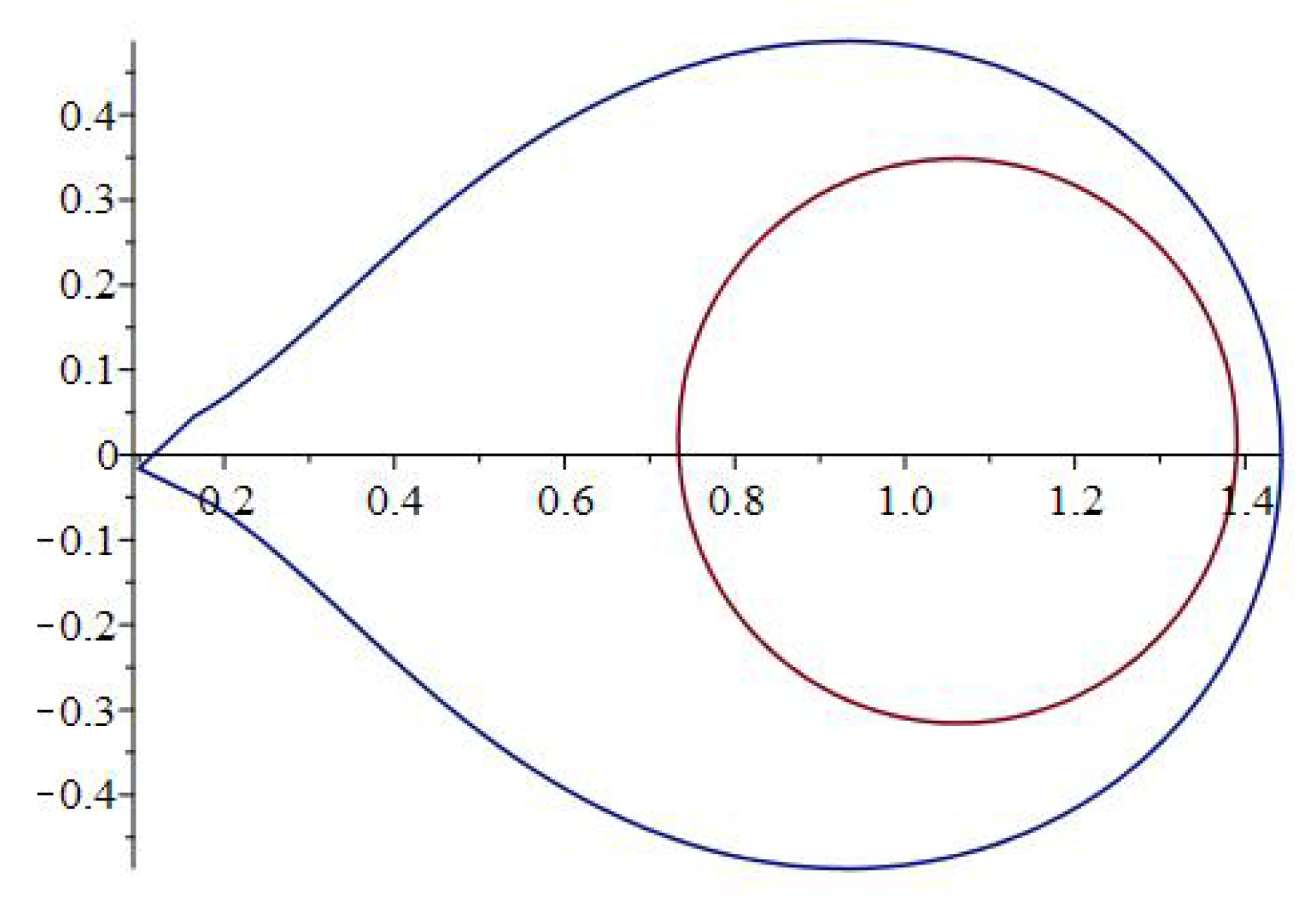
Using the notations of the Definition 3 it is easy to check that for all , hence . Taking the particular case , , and using the 2D plot of the MAPLE™ computer software we obtain the image of the boundary by the functions Θ, Λ and presented in the Figure 4. Since the function is univalent in , hence the subordinations and hold because , and (see Figure 4). Hence , therefore the class is not empty and contains other functions than the identity.
In the following theorem we will determine the results for the initial coefficients bounds of the class .
Theorem 5.
If is given by (1), then
and
Proof.
If , from the Definition 3 there exist two analytic functions in , namely u and v such that and , for all , with
With the same notations like in the proof of the Theorem 3, from the equalities (43) and (44) we obtain that
and
If we add (48) and (50) we get
and substituting the value of from (52) in the right hand side of (53) we deduce that
hence
Using (5) of Lemma 1 and the triangle’s inequality in (52) and (54) we obtain
that proves our first inequality.
Using again Lemma 1 and the triangle’s inequality it follows that
To determine the upper bound of the Fekete–Szegő functional for the class we will use the following lemma:
Lemma 3.
[24, (3.9), (3.10) p. 254] If , with , then there exist some x, ζ with , , such that
Theorem 6.
If is given by (1), then
Proof.
With the same notations like in the proof of the Theorem 3, from Lemma 3 we have and , , , and using (51) we get
hence
Using the triangle’s inequality, taking , , , and without losing of generality we can assume that , , thus we obtain
Denoting and the above relation could be rewritten in the form
Thus,
and substituting the value and in the above last equality we obtain
Now we will determine the maximum of H on . Since
it is clear that if and only if . In this case function H is a decreasing function on , therefore
Also, if and only if , hence the function H is an increasing function on , and consequently
and the estimation (56) is proved. □
5. Conclusions
In our present investigation we have introduced and studied the initial coefficient problems associated with each of the new subclasses , and of the well-known bi-univalent class . These bi-univalent function subclasses are given by Definitions 1 2, and 3 respectively. For the functions in each of these bi-univalent subclasses we have obtained the estimates of the Taylor–Maclaurin coefficients and , and we gave solutions for the Fekete-Szegő functional problems. New results are shown to follow upon specializing the parameters involved in our main results as given in Remark 2 for the class of bi-starlike and bi-convex functions associated with Gregory coefficients which are new and not yet studied sofar. Further we can extend these type of studies based on generalized telephone numbers (see [25,26,27]).
Author Contributions
For research articles with several authors, a short paragraph specifying their individual contributions must be provided. The following statements should be used “Conceptualization, G.M., K.V. and T.B.; methodology G.M., K.V. and T.B.; software, G.M., K.V. and T.B.; validation, G.M., K.V. and T.B.; formal analysis, G.M., K.V. and T.B.; investigation, G.M., K.V. and T.B.; resources, G.M., K.V. and T.B.; data curation, G.M., K.V. and T.B.; writing—original draft preparation, G.M., K.V.; writing—review and editing, G.M., K.V. and T.B.; visualization, G.M., K.V. and T.B.; supervision, G.M., K.V. and T.B.; project administration, G.M., K.V. and T.B. All authors have read and agreed to the published version of the manuscript.
Funding
This research received no external funding.
Data Availability Statement
Not applicable.
Acknowledgments
The authors are grateful to the reviewers of this article that gave valuable remarks, comments, and advice in order to improve the quality of the paper.
Conflicts of Interest
The authors declare no conflict of interest.
References
- Lewin, M. On a coefficient problem for bi-univalent functions. Proc. Amer. Math. Soc. 1967, 18, 63–68.
- Brannan, D.A.; Clunie, J.G. Aspects of contemporary complex analysis. In Proceedings of the NATO Advanced Study Institute held at the University of Durham, Durham, July, 1979, Academic Press, New York and London, 1980.
- Netanyahu, E. The minimal distance of the image boundary from the origin and the second coefficient of a univalent function in |z| < 1. Arch. Ration. Mech. Anal. 1969, 32, 100–112.
- Brannan, D.A.; Taha, T.S. On some classes of bi-univalent functions, Studia Univ. Babeş-Bolyai Math. 1986, 31(2), 70–77.
- Taha, T.S. Topics in Univalent Function Theory, PhD. Thesis, University of London, 1981.
- Srivastava, H.M.; A.K. Mishra; Gochhayat, P. Certain subclasses of analytic and bi-univalent functions. Appl. Math. Lett. 2010, 23(10), 1188–1192.
- Bulut, S. Coefficient estimates for a class of analytic and bi-univalent functions. Novi Sad J. Math. 2013, 43, 59–65.
- Frasin, B.A.; Aouf, M.K. New subclasses of bi-univalent functions. Appl. Math. Lett. 2011, 24, 1569–1573.
- Murugusundaramoorthy, G.; Magesh, N.; Prameela, V. Coefficient bounds for certain subclasses of bi-univalent function. Abstr. Appl. Anal. 2013, Volume 2013, Article ID 573017, 3 pages.
- Srivastava, H.M.; Murugusundaramoorthy, G.; El-Deeb, S.M. Faber polynomial coefficient estimates of bi-close-convex functions connected with the Borel distribution of the Mittag-Leffler type. J. Nonlinear Var. Anal. 2012, 5(1), 103–118. [CrossRef]
- Srivastava, H.M.; Murugusundaramoorthy, G.; Bulboacă, T. The second Hankel determinant for subclasses of bi-univalent functions associated with a nephroid domain. Rev. R. Acad. Cienc. Exactas Fs. Nat. Ser. A Mat. RACSAM 2022, 116, Article ID: 145, 1–21. [CrossRef]
- Srivastava, H.M.; Eker, S.S.; Ali, R.M. Coefficient bounds for a certain class of analytic and bi-univalent functions. Filomat 2015, 29(8), 1839–1845.
- Srivastava, H.M.; Sakar, F.M.; Güney, H.Ö. Some general coefficient estimates for a new class of analytic and bi-univalent functions defined by a linear combination. Filomat 2018, 32(4), 1313–1322.
- Yousef, F.; Amourah, A.; Frasin, B.A.; Bulboacă, T. An avant-garde construction for subclasses of analytic bi-univalent functions. Axioms 2022, 11(6), 267. [CrossRef]
- Fekete, M.; Szegő, G. Eine Bemerkung Über Ungerade Schlichte Funktionen. J. Lond. Math. Soc. 1933, 1-8(2), 85–89.
- Phillips, G.M. Gregory’s method for numerical integration. Amer. Math. Monthly 1972, 79(3), 270–274.
- Berezin, I.S.; Zhidkov, N.P. Computing Methods, Pergamon, North Atlantic Treaty Organization and London Mathematical Society, 1965.
- Cantor, D.G. Power series with integral coefficients. Bull. Amer. Math.Soc. 1963, 69(3), 62–366.
- Zaprawa, P. On the Fekete-Szegő problem for classes of bi-univalent functions. Bull. Belg. Math. Soc. Simon Stevin 2014, 21(1), 169–178.
- Zaprawa, P. Estimates of initial coefficients for bi-univalent functions. Abstr. Appl. Anal. 2014, Article ID: 357480. [CrossRef]
- Carathéodory, C. Über den Variabilitätsbereich der Koeffizienten von Potenzreihen, die gegebene Werte nicht annehmen. Math. Ann. 1907, 64(1), 95–115.
- Pommerenke, C. Univalent Functions, Vandenhoeck and Ruprecht, Göttingen, 1975.
- Duren, P.L. Univalent Functions, Springer, Amsterdam, 1983.
- Libera, R.J.; Zlotkiewicz, E.J. Coefficient bounds for the inverse of a function with derivative in P. Proc. Amer. Math. Soc. 1983, 87(2), 251–257.
- Murugusundaramoorthy, G.; Vijaya, K. Certain subclasses of snalytic functions associated with generalized telephone numbers. Symmetry 2022, 14(5), 1053. [CrossRef]
- K. Vijaya; Murugusundaramoorthy, G. Bi-starlike function of complex order involving Mathieu-type series associated with telephone numbers. Symmetry 2023, 15(3), 638. [CrossRef]
- Deniz, E. Sharp coefficient bounds for starlike functions associated with generalized telephone numbers. Bull Malays. Math. Sci. Soc. 2021, 44, 1525–1542.
Figure 1.
The image of .
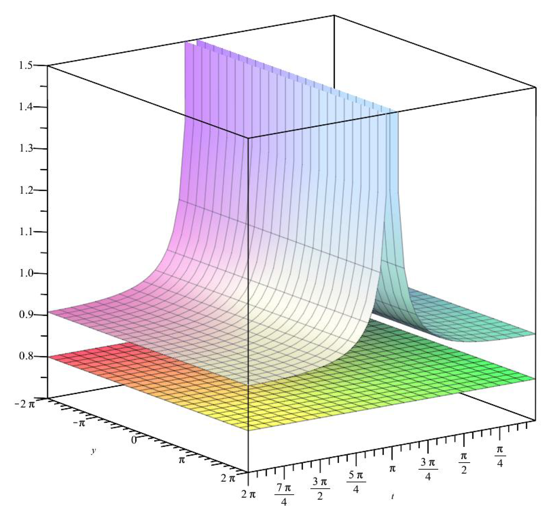
Figure 2.
The images of , (blue color) and (red color), .
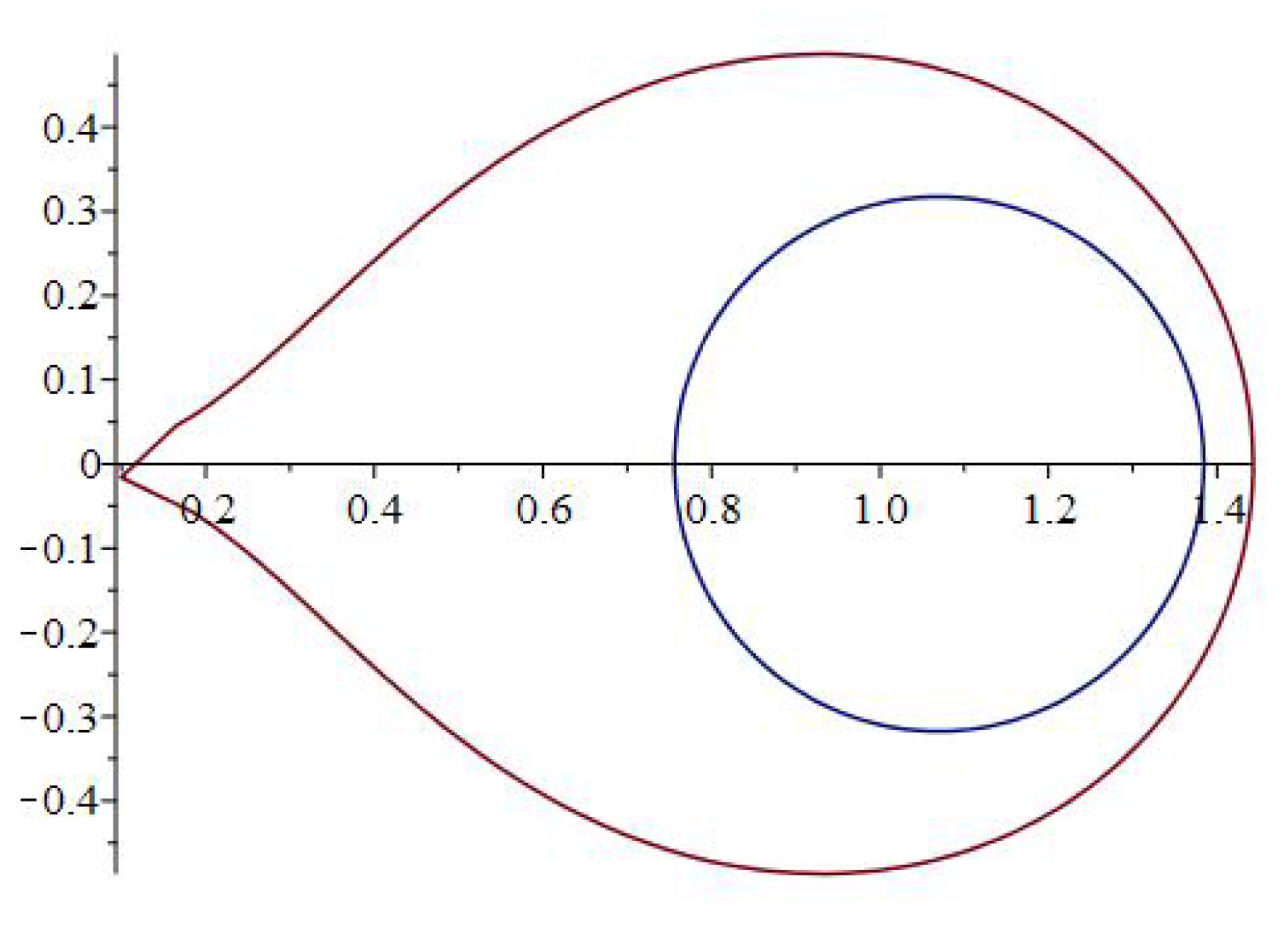
Figure 3.
The images of , (red color) and (blue color), .
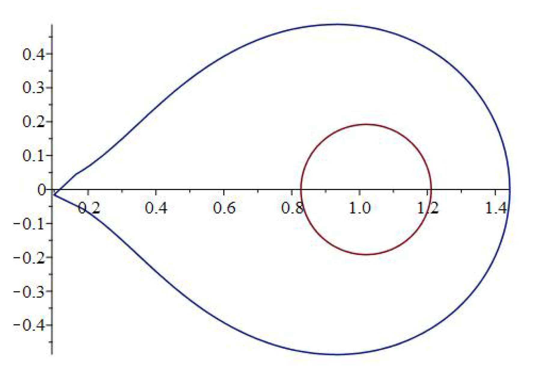
Figure 4.
The images of , (red color) and (blue color), .
Disclaimer/Publisher’s Note: The statements, opinions and data contained in all publications are solely those of the individual author(s) and contributor(s) and not of MDPI and/or the editor(s). MDPI and/or the editor(s) disclaim responsibility for any injury to people or property resulting from any ideas, methods, instructions or products referred to in the content. |
© 2020 by the authors. Licensee MDPI, Basel, Switzerland. This article is an open access article distributed under the terms and conditions of the Creative Commons Attribution (CC BY) license (https://creativecommons.org/licenses/by/4.0/).
Copyright: This open access article is published under a Creative Commons CC BY 4.0 license, which permit the free download, distribution, and reuse, provided that the author and preprint are cited in any reuse.


