Submitted:
15 May 2023
Posted:
16 May 2023
You are already at the latest version
Abstract
This paper presents a cascade predictive control structure based on the field-oriented control (FOC) in the dq rotor reference frame for the synchronous reluctance machine (SynRM). The constant d-axis current control strategy was used and thus, the electromagnetic torque was directly controlled by the q-axis current. Because the model of the two axes currents from the inner loop is a coupled non-linear multivariable one, to non-interaction linear control the two currents, their decoupling was achieved through feedforward components. Following the decoupling, two independent monovariable linear systems resulted for the two currents dynamics that were controlled using model predictive control (MPC) algorithms, considering their ability to automatically handle the state bounds. The most important bounds for SynRM are the limits imposed on currents and voltages, which in the dq plane correspond to a circular limit. To avoid computational effort, linear limitations were adopted through polygonal approximations, resulting in rectangular regions in the dq plane. For the outer loop that controls the angular speed with a constrained MPC algorithm, as plant was considered the q-axis current closed loop dynamics and the torque linear equation. To evaluate the performances of the proposed cascade predictive control structure, a simulation study using MPC controllers versus PI ones was conducted.
Keywords:
synchronous reluctance machine
; model predictive control
; field orientation control
; linear constraints
; quadratic programming
1. Introduction
The high performance electric drive systems are now designed to fulfill the main requirements such as fast transient, high power density, high efficiency, low rotor inertia. On a large scale, the most popular used electric machine is the induction one, but with low efficiency for low power range, which makes it to be inappropriate for this kind of application. A secondary option is represented by the permanent magnet synchronous machine with various benefits as high efficiency and low rotor inertia, but with the main drawback given by the demagnetization phenomenon when operating at high temperatures. At last, the synchronous reluctance machine (SynRM) becomes an attractive solution for a large range of power and speed, being a low-cost machine with eco-friendly environment impact, and multiple benefits, as: compact sizes, low mass and rotor inertia, and the rotor having no electric windings, cage, or permanent magnets. For the modern applications of SynRM drives, advanced control algorithms are used to obtain high performances such as fast transient regime, good tracking results, efficient disturbance rejection [1,2].
The main control strategies of SynRM are divided into the following categories: constant d-axis current control (when the torque is varied by the q-axis current), current angle control (with the groups: fast torque response, maximum power factor control, maximum torque per ampere control) and active flux control [4,5]. These control strategies are usually implemented using the field-oriented control (FOC) concept, which involves a cascade control structure with an outer loop for angular speed control and an inner loop for d-axis and q-axis currents control. To control the d-axis and q-axis currents independently, decoupling feedforward components are frequently used in both current control loops.
For FOC approach, simple control solutions, such as proportional–integral (PI) controllers are dominant in many applications but having as main drawback the inability to deal with constraints in a nonconservative way. For example, a cascade structure based on FOC that uses the constant d-axis current strategy whose two loops controllers are PI is given in [6]. In [4], the performances obtained with PI controllers are comparatively analyzed for the main control strategies of SynRM implemented in a cascade control structure based on FOC. With a constant d-axis current reference, in [7] a FOC strategy with PI controllers having an anti-wind-up mechanism is used to develop a cascade control structure for SynRM.
The current control problem of the SynRM is a quadratically constrained problem and for this reason, a solution was the use of model predictive control (MPC) algorithms that can automatically handle the constraints. However, at the beginning the main problem in using MPC algorithms for SynRM control was the computational complexity. In recent years, with the advances in hardware and solver development, MPC strategy can be successfully implemented in SynRM control systems. For the predictive current control, based on the way in which the switching action of the power inverter is produced, the finite set or continuous set approach is used. Thus, in [8], a current predictive control algorithm for a finite set of switching actions of the power inverter was introduced based on a one-step-ahead prediction model obtained by the discretization of the continuous time coupled non-linear multivariable dq current model with the forward Euler method. Using a cost function with soft constraints, the optimal switching vector for the inverter was selected. A similar current predictive control algorithm is presented in [9], considering a coupled linear multivariable dq current model by using a constant rotor electrical angular speed. The overcurrent protection is obtained by adding a variable in the cost function that considers the safety current limits. Recently, model-free MPC current controllers have been developed. Thus, this approach is presented in [10] using a model-free MPC current controller based on a finite-set unconstrained approach. For current prediction, current measurements continually updated stored in a look-up table are employed. A similar approach, where an improved unconstrained model-free MPC current control based on a flux-current map of SynRM for considering the nonlinear magnetic features of SynRM can be found in [11]. At the same time, in [12] an unconstrained continuous-set model-free MPC algorithm without using the explicit model of SynRM is introduced.
Starting from the multivariable model of dq currents and the monovariable one obtained by decoupling, in [13] MPC current controllers with constraints based on continuous set approach are designed and their performances are compared.
For the outer loop, meant to control the angular speed of SynRM, the PI controller is the most frequently used [3,4], [6,7]. Due to the difficulty of this controller regarding constraints handling, MPC algorithms are also used for speed control [14].
Although, the MPC with finite set control is widely used in SynRM control due to certain benefits in SynRM control [7], the high switching frequency required by this strategy [15,16] reduces the performances of the practical applications, becoming an impediment for real-time implementation. At the same time, for MPC with finite set control strategy, the constraints handling is difficult. The overcurrent protection is usually obtained by adding a soft constraint set in the cost function that considers the safety current limits, while the voltage limitations are directly imposed by the searching algorithm which generates a voltage magnitude in the admissible domain.
Regarding the continuous set approach used for field oriented predictive control of SynRM, according to the authors' knowledge, few results have been reported. Thus, in [18] the design and implementation of a current controller for a SynRM based on the continuous set nonlinear model predictive control is described. For a permanent magnet assisted synchronous reluctance motor (PMA-SynRM), starting from nonlinear dynamical model in [19], the design of a continuous set MPC based on an augmented linearized model is presented.
In this paper a cascade predictive control structure based on FOC in dq rotor reference frame for SynRM was proposed. Among the FOC-based SynRM control strategies, the constant d-axis current control was chosen, which provides the direct control of the electromagnetic torque through the q-axis current. Because the model of the two axes currents from the inner loop is a coupled non-linear multivariable one, to non-interaction linear control the two currents, their decoupling was achieved through feedforward components. In this way, the dynamics of the d-axis current, which must be constant, is not influenced by the q-axis current variations. After decoupling, two independent monovariable linear systems resulted for the two currents dynamics that were controlled using MPC algorithms, due to their ability to automatically handle the bounds imposed on the states.
The most important bounds for SynRM are the limits imposed on currents and voltages, which in the dq plane correspond to circular regions. To avoid computational effort, linear limitations were adopted through polygonal approximations, resulting in rectangular regions in the dq plane. For the d-axis current, the upper limit was imposed as its reference, and thus, the parameter of the circular region transformation related to the currents into a rectangular one was defined by the ratio between the d-axis current reference and the maximum stator current. The transformation of the circular region related to the voltages into a rectangular one in the dq plane was carried out by a parameter chosen by the user. To obtain the constraints imposed on the outputs of the MPC current controllers, the voltage limitations in the dq plane were considered, to which the maximum values of the feedforward components were appropriately added. For the outer loop that controls the angular speed with a constrained MPC algorithm, it was considered as plant the q-axis current closed loop dynamics and the linear equation of the torque depending on the q-axis current. To eliminate the steady state speed error due to unmeasured disturbance generated by the load torque and modeling errors, the user speed reference of the MPC speed controller is replaced by adding an integral action and a feedforward component.
The MPC algorithms were designed in such a way to obtain reference tracking by adding an additional state to the plant model to obtain input increment which becomes optimization variable. The cost functions and related constraints used for MPC algorithms design were transformed into a quadratic programming (QP) problem. To avoid the infeasibility of the QP problem, some constraints are treated as soft constraints by using a slack variable. The implementation is done in Matlab-Simulink using the facilities offered by the MPC Designer from Model Predictive Control Toolbox. To evaluate the performance of the proposed cascade predictive control structure based on FOC in the dq rotor reference frame for SynRM, a simulation study using MPC controllers versus PI ones was conducted. PI controllers, often used for the cascade control of SynRM in industrial applications, were designed using the pole-placement method, and to limit some variables imposed by the constraints, saturation type blocks were introduced at the output of the controllers together with the related anti-windup mechanisms. Since the design method introduces a zero in the closed loop system, a zero-cancelation ZC block was used in order not to alter the performances. Finally, through a comparative analysis of the performances obtained with the MPC and ZC-PI controllers respectively, the better performing behavior of the predictive control cascade structure resulted.
The rest of the paper is organized as follows. In Section II the dq SynRM model with physical limits together with the cascade predictive control structure in the dq rotor reference frame are presented. Section III is dedicated to the design of the inner and outer loops of the proposed cascade predictive control structure. A comparative analysis of the performances obtained with the MPC and ZC-PI controllers is given in Section IV. The conclusions of the paper are presented in Section V.
2. SynRM cascade predictive control structure in the rotor reference frame
In this paper, a cascade predictive control structure is proposed for SynRM currents and angular speed control in the rotor reference frame.
2.1. Plant model and physical limits
The dq SynRM model is composed of the electrical circuit, torque generator and mechanical system models [3]. The electrical circuit is described by the current equations:
where (ud,uq), (id,iq), and (Ld,Lq) are voltages, currents and inductances on the d-axis and q-axis, and Rs is the stator resistance. The torque generator is described by the following equation:
and the equation of the mechanical system is given by:
where (ωe,ωm) denote the electrical and mechanical speeds, with , p being the number of poles pairs, and (Te,Tl) denote the electromagnetic and load torques.
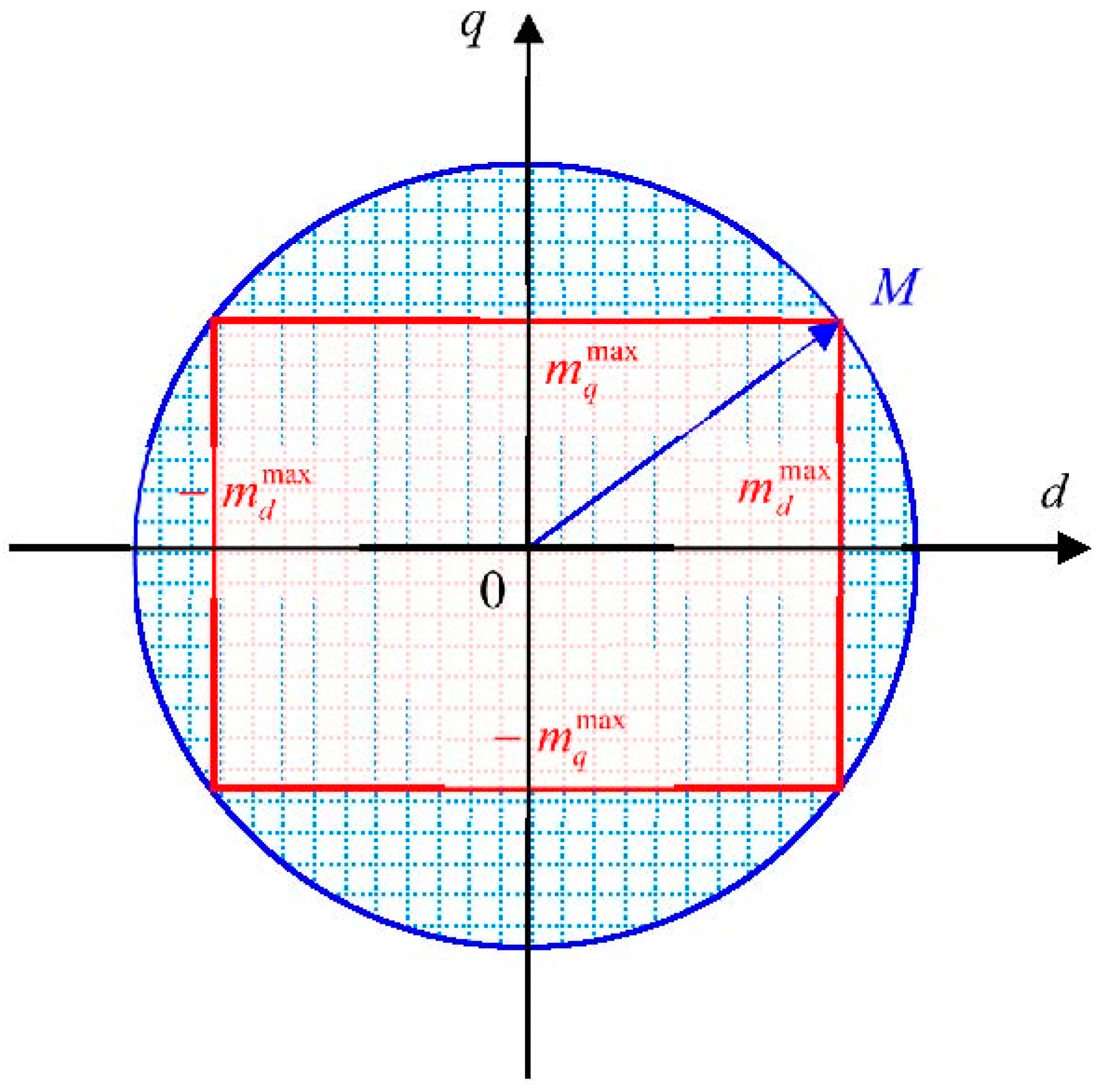
The electrical circuit model (1) of the SynRM is multivariable and non-linear as it includes the product of the electrical angular velocity and the dq currents. In the same time, critical constraints are imposed on the electrical variables, the most important referring to the limitation of currents and voltages whose upper limits on the magnitude correspond to a circular limit in the dq plane. Using the generic notation for current and voltage signals, the main constraint becomes:
where M is the maximum phase amplitude of the stator current , respectively, of the stator voltage . Typically is determined from the motor specifications and if the space vector pulse-width modulation is used for the inverter control with DC-link voltage , . Due to the high computational effort imposed by the circular limit (4), its approximation through linear polygonal limitations was chosen. Thus, the circular region is approximated by a rectangular one defined by the maximum values [19]:
where is a parameter that determines the configuration of the rectangular region. Using limits (5), the linear constraints become:
The circular and the rectangular regions are represented in Figure 1, from where it can be seen that the rectangular area is smaller than the circular one.
Figure 1.
The rectangular approximation of the circular region.
The torque generator model (2) is also non-linear due to the product of the two currents. Usually, for the mechanical system, a constraint is imposed on the angular speed limits of the motor:
In the following, to simplify the notations, the time variable t will be omitted.
2.2. Cascade predictive control structure
Using the electrical circuit, the torque generator and the mechanical system models (1), (2) and (3), the cascade predictive control structure of a SynRM in the rotor reference frame from Figure 2 was developed for the currents and the motor angular speed control. Since the dynamics of the mechanical system are slower compared to the electrical ones, the outer loop is intended for mechanical speed regulation and the inner one for dq currents control. For both loops, MPC was chosen as the control laws due to the superior performance obtained and the possibility of considering in the design phase the constraints originating from physical limits.
Among the cascade control strategies of SynRM, the one based on keeping constant the current on the d-axis was chosen [20]. In this way, the current on the q-axis will be the one that controls the electromagnetic torque and relation (2) becomes a linear one.
The inner loop has as a plant the multivariable and non-linear model of the electrical circuit (1). The plant model is decoupled using the feedforward control components from Decoupling block, resulting in two linear monovariable systems that are controlled with MPCd and MPCq controllers whose output variables are and . The first monovariable system will control the current for which the constant reference is imposed, and the second one, the current for which the reference is generated by the outer loop controller. Considering the possibility to treat the state bounds by the MPC controllers intended for the inner current loop, the linear constraints (6) adapted to the currents - and the voltages - will be used.
Figure 2.
The cascade predictive control structure.
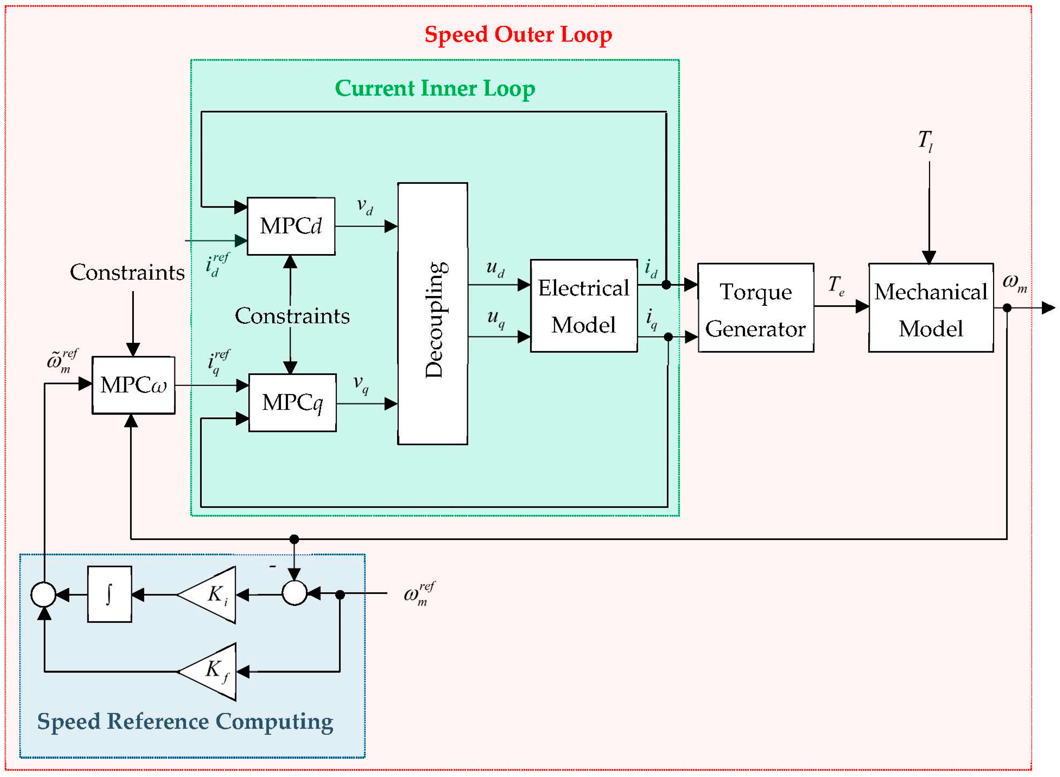
For the outer loop, the plant is composed of the inner loop for the current control because the current is considered constant, of the torque generator and the mechanical system. By adopting the control strategy based on keeping constant the d-axis current, the outer plant is a linear one that will be controlled by the MPCω controller. To eliminate the steady state error due to unmeasured disturbance generated by the load torque and modeling errors, an integral action and a feedforward component with the gains and are added for the offset-free tracking. Thus, the reference of the MPCω controller will be replaced by [21]:
where the gains and are chosen in such a way as to influence the dynamics of the control system as little as possible. The outer loop controller will limit the angular speed by using the linear constraint (7).
3. Design of the cascade predictive control structure
The design of the proposed cascade predictive control structure from Figure 2 consists in solving the control problems of the two loops. Firstly, the feedforward control components and the MPCd and MPCq controllers related to the inner loop are designed for controlling the and currents considering the constraints imposed by the physical limits. Secondly, the MPCω controller related to the outer loop is designed to control the angular speed of the motor in the presence of the load torque and constraints.
3.1. Inner current loop design
Considering the control problems imposed to the internal loop, the control structure from Figure 3 was chosen.
Figure 3.
The inner current loop control structure of SynRM.
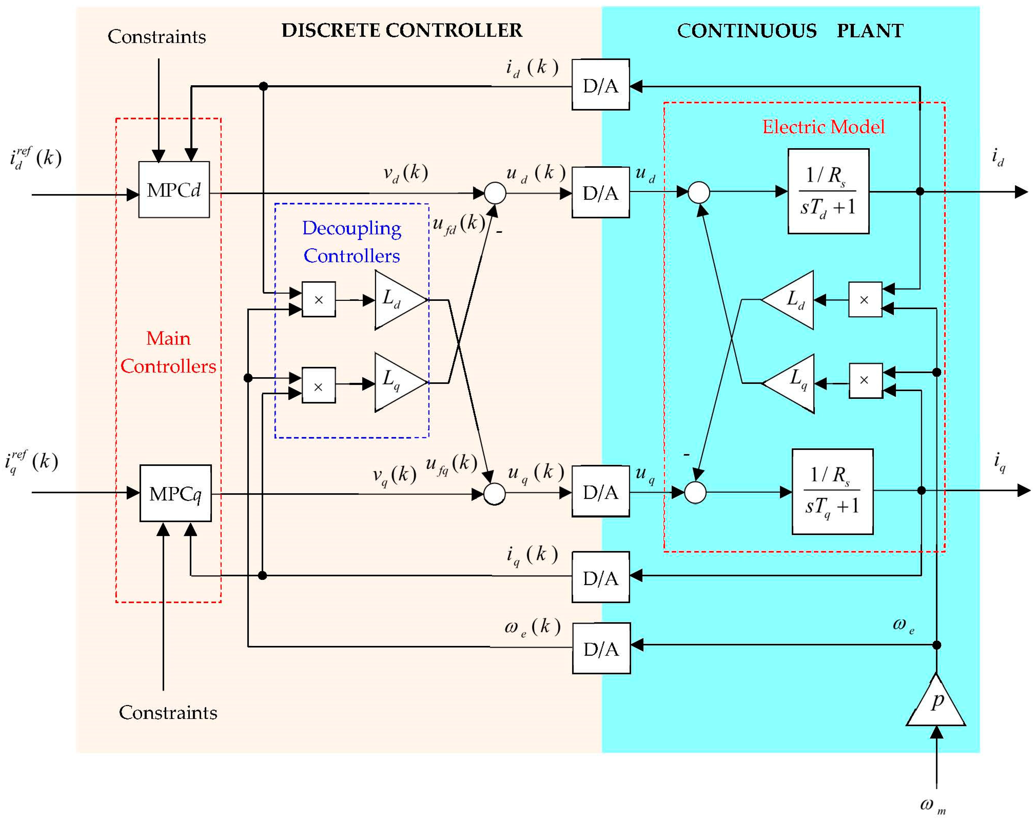
The plant is described by equation (1) which highlights a non-linear multivariable system whose main channels are described by the transfer functions of the R-L circuits:
where are the time constants of R-L circuits. Considering that both the feedforward components and the MPCd/q predictive controllers are discrete-time type, for their design, model (1) is discretized with the forward Euler method resulting in:
for which the following notations were used:
The first two terms of the right side of equation (10) represent the discrete-time model of the R-L circuit, and the last term, the interaction between the channels of the multivariable system. To eliminate the interactions containing nonlinearities, feedforward components are used described by:
resulting for the voltages uj the expressions:
where vj represents the input variables of the two decoupled monovariable R-L circuits.
Replacing uj given by (13) in (10), the decoupled monovariable discrete-time models are obtained:
that will become plants for MPCd/q controllers.
For the currents to track their references , the increment:
is considered as input signal, the reason for which the model (10) is extended with the new state , resulting the augmented model:
Using the compact form of the model (16):
the linear prediction model can be easily determined:
and finally, the output prediction:
Considering the linear constraints (6) imposed on the electrical variables, in the following they will be specified for the currents ij and the voltages vj. Thus, for the currents, the maximum values result:
where ci is a parameter that fixes the maximum value of the stator current according to the nominal value . Knowing that the id current is positive and upper limited by , the parameter will be and the current linear constraints related to (6) and (5) become:
The constraints imposed on the vj voltages depend on the uj voltage constraints generated by the physical limitations and the relationships (13) between vj and uj. First, the maximum values of the uj voltages are determined based on equation (5):
and then, the maximum values of the feedforward components ufj are determined using the maximum values of the currents ij and the nominal electrical angular velocity :
Introducing the maximum values of the voltages uj and ufj in (13), the maximum values of the voltages vj are obtained:
and thus, the linear constraints related to the control signals of the two MPC current controllers are found:
Considering the tracking of the references by the currents , the constrained quadratic cost function is chosen having the form:
where is the future control sequence, hpj and hcj are the prediction and control horizons, δjn and λjp are the real positive weights factors of the output and the control signals. The slack variable is introduced to allow constraints violations together with the nonnegative weights and , while the term is added to penalize in the cost function with .
The constrained quadratic cost function (26), by substituting the output prediction (19) can be reformulated as a QP problem which leads to the optimal solution [22]:
where the involved matrices Hj, Fj, Gj, Wj and Sj of adequate sizes are determined as in [23].
According to the receding horizon principle, only the first element of is used to determine the control signal applied to the decoupling controller:
Since the strategy of keeping the id current constant was considered, the reference for the current control loop was chosen based on the active flux concept [24]:
and thus, the electromagnetic torque of the SynRM motor is given now by the linear relationship:
which replaces the non-linear expression (2) of the torque.
3.2. Outer speed loop design
For the outer loop, the plant consists of the designed inner closed-loop system of the iq current to which the mechanical system model (3) is added considering the electromagnetic torque (30). Usually, the dynamics of the inner closed-loop system of the iq current is approximated with a first-order element whose time constant is correlated with the closed-loop dynamics:
Based on the two models (31) and (3) with the electromagnetic torque (30) , the outer loop plant model having as input um the reference and as output the mechanical speed is described by:
where the following notations were used:
To obtain output free tracking, a new state is added to the system states (32), resulting the augmented model:
For the augmented model (34), the input is the increment and thus will track the reference . Considering a zero-load disturbance , the model (34) can be put in its compact form:
based on which the linear prediction model is simply determined:
Using (36), the output prediction is directly found:
Having in view the necessity to track the reference by the controlled output and the limitations regarding the controlled output and the input signal , a quadratic constrained cost function of the form was chosen:
where is the future control sequence, hpm and hcm are the prediction and control horizons, is the slack variable used to relax the constraints together with the nonnegative weights , δjm and λjm are the real positive weights factors of the output and the control signals, is the slack variable weight, are the limits of the speed. Since , are chosen according to the second inequality from (21).
The quadratic cost function (38) subjects to the linear constraints can be reformulated as a QP problem by substituting the output prediction (37), which leads to the optimal solution [22]:
where the involved matrices Hm, Fm, Gm, Wm and Sm of adequate sizes are determined as in [23].
Based on the receding horizon principle, only the first element of is used to determine the control signal applied to the inner control loop of the current as reference:
4. Illustrative case study
To evaluate the performances of the proposed cascade predictive control structure for SynRM, a simulation study was carried out using a Simulink model of the motor in dq coordinates and predictive controllers from the MPC Simulink Library.
The simulation results were compared with those obtained with a cascade regulation structure with ZC-PI controllers instead of MPC ones, often used in industrial applications. For the design of the PI controllers, the pole placement method was used [25], considering the R-L plant transfer function for the current controllers:
and the mechanical plant transfer function for the speed controller, neglecting the inner loop dynamics:
Following the design of the PI controllers, the tuning parameters of the current and speed controllers resulted:
where is the natural frequency and is the loop attenuation of the inner/outer loop systems. Furthermore, a zero appears in the closed–loop transfer function which can be canceled by introducing a zero–cancellation block ZC in the feedforward path [25].
The saturation used for ZC-PI controllers output constraints requires an anti-windup mechanism [26].

Table 1.
SynRM specifications.
| Symbol | Description | Values |
|---|---|---|
| PN [W] | Nominal power | 3000 |
| UN [V] | Nominal voltage | 355 |
| TN [Nm] | Nominal torque | 19.1 |
| ψaN [Wb] | Nominal active flux | 0.69 |
| IN [A] | Nominal current | 7.9 |
| ωmN [rad/sec] | Nominal speed | 157 |
| Rs [Ω] | Rotor resistence | 1.35 |
| Ld [H] | Direct axis inductance | 0.186 |
| Lq [H] | Quadrature axis inductance | 0.04 |
| J[kg∙m2] | Rotor inertia | 0.079 |
| p | Stator pole pairs | 2 |
| UDC [V] | Nominal DC link voltage | 650 |
The sampling period for the controller design was chosen Ts = 50 microseconds according to the requirements of the current loops’ dynamics.
With the SynRM parameters from Table 1, the inner plant model used for MPC current controllers design turns into:
and the outer plant model including inner loops dynamics for MPC speed controller design becomes:
The simulation study is performed in Matlab-Simulink environment, by using the MPC Designer block from Model Predictive Control Toolbox. Since the control strategy based on keeping constant the current on the d-axis was chosen for the cascade predictive control structure of SynRM, the reference for id is calculated with [27].
The limit values of the constraints were determined based on the method from Section 2, using the rectangular regions from Figure 1. The circle radius M for currents is given by and for voltages by . Since for the constant current on the d-axis, the limitation is imposed, the value was adopted. For the voltages uj constraints, was assumed, and for vj voltages, equations (24-25) were used to obtain the imposed limitations.
For the speed reference computing, the following gains values are selected: and .
Thus, Table 2 summarizes the tuning parameters and constraints for both MPC and PI controllers.
Table 2.
Tuning parameters and constraints for controllers of the two cascade structures.
| Controller | Parameter | Current loops | Speed loop (m) |
|
| j=d | j=q | |||
| MPC | δj/m | 0.6 | 0.5 | 0.7 |
| λj/m | 10-5 | 3∙10-5 | 2∙10-5 | |
| hpj/m | 40 | 40 | 20 | |
| hcj/m | 2 | 2 | 2 | |
| uj/mmin/max | -/+112.58V | -/+356.51V | - /+9.98A | |
| vjmin/max | -/+237.99V | -/+78.75V | - | |
| id/qmin/max | 0/4.75 | -/+9.98A | - | |
| Vj/mmin | 0A | 0A | 0rad/sec | |
| Vj/mmax | 1A | 1A | 1rad/sec | |
| 105 | 105 | 105 | ||
| ZC-PI | Kpj/m | 4.05 | 1.34 | 0.51 |
| Kij/m | 78.41 | 91.09 | 0.21 | |
| vjmin/max | -/+237.99V | -/+78.75V | - | |
| ummin/max | - | - | - /+9.98A | |
The outer speed loop tracking results for both MPC and ZC-PI controllers of SynRM cascade structure are depicted in Figure 4. The speed reference is set at a constant value that corresponds to the nominal one . A no-load start of SynRM is considered, and then, after 4 sec a load torque of value is applied (Figure 6), which represents the main disturbance that acts on SynRM. As it can be seen in Figure 4, for the MPC control is obtained the settling time , which is much smaller than the settling time achieved with ZC-PI control. Additionally, ZC-PI speed control response has a very small overshoot, while MPC speed control has no overshoot.
Figure 4.
The speed tracking results.
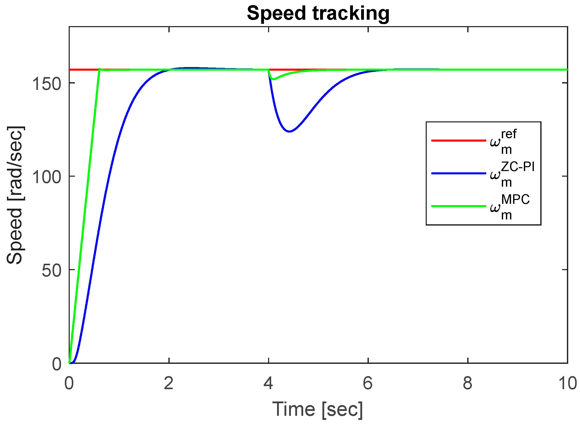
Moreover, when the load torque is applied, the speed variations are much higher with ZC-PI control compared to MPC. It can be mentioned, that on the no-load start conditions of SynRM, the fast outer speed closed loop dynamics with MPCω generates a high value of the controller output, which will be limited by the imposed constraints. The same limitation is also applied as q-axis current reference. Therefore, the current references and their tracking, which are presented in Figure 5 have a major influence of SynRM operation.
Figure 5.
The inner current loop tracking results.
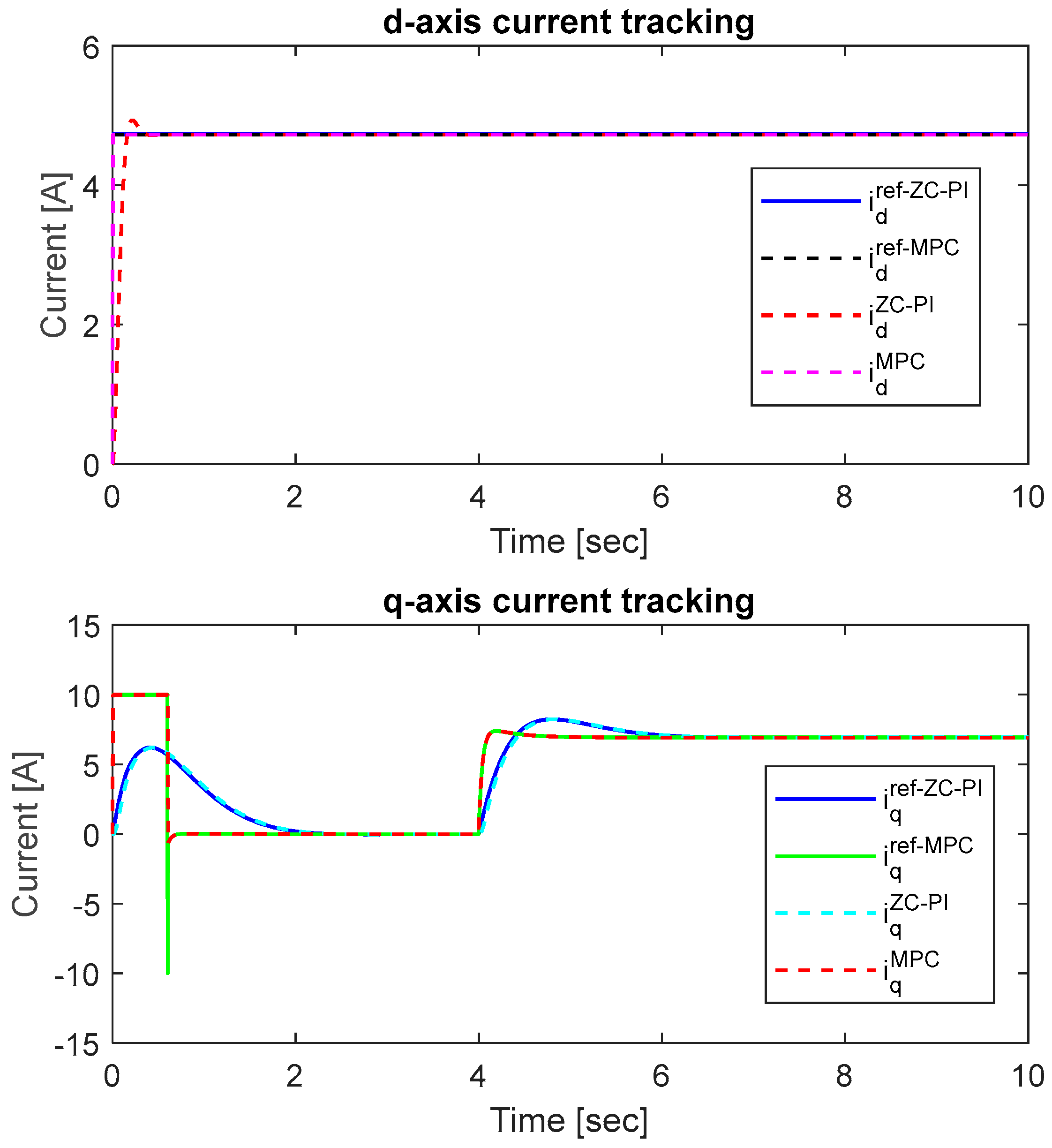
The currents constraints are established according to Table 2. For d-axis, the MPC current response is faster than the corresponding ZC-PI one . Moreover, compared with ZC-PI current response, the MPC current response presents no overshoot. On the q-axis, both current responses, and , must track their current references which are provided by the speed controller. At the start of SynRM drive, the q-axis MPC current response has a larger value than the ZC-PI one and is limited by the constraints. When the load torque is applied (Figure 6), the response is faster than the ZC-PI one , and both responses present small overshoots.
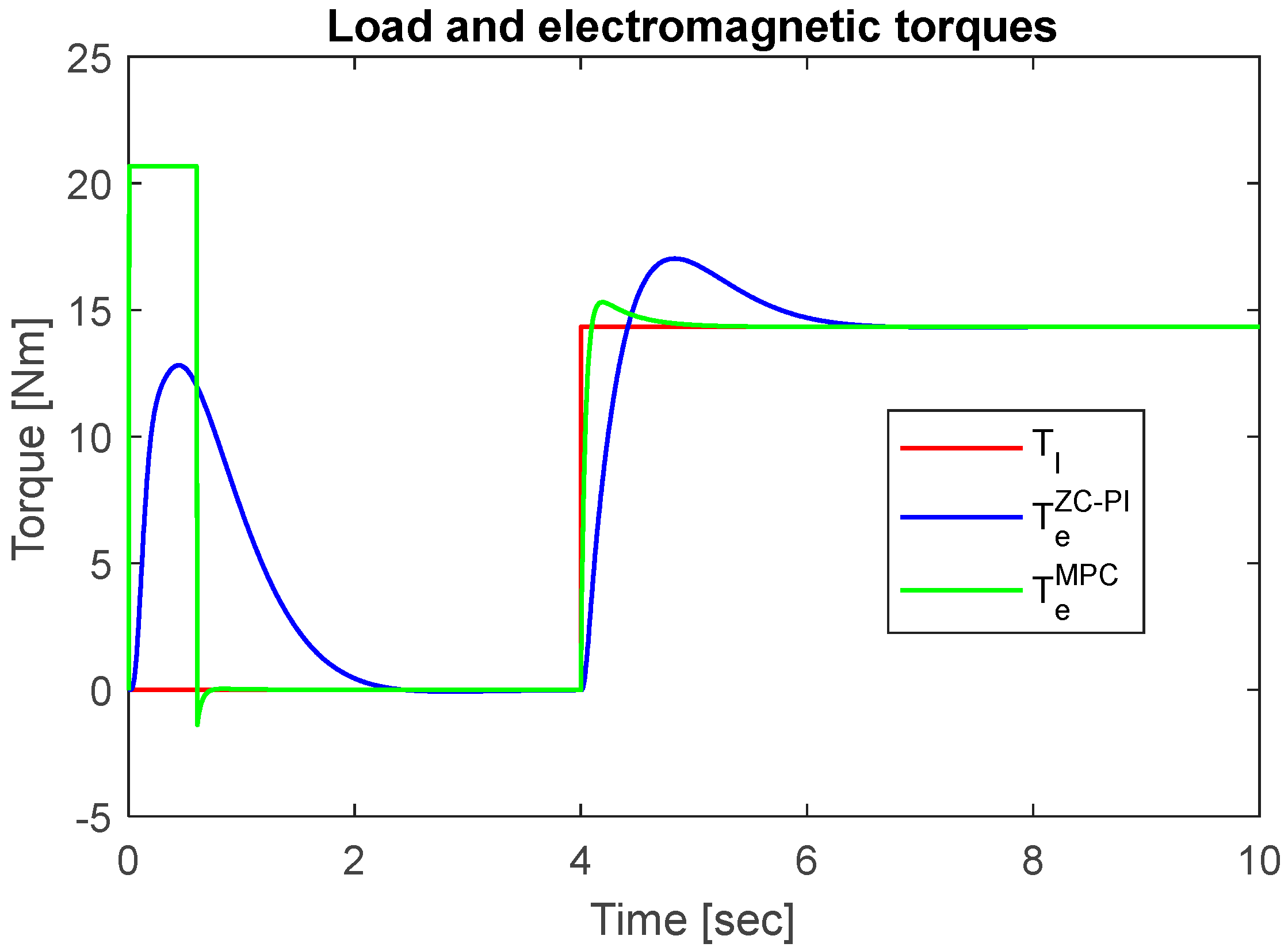
The electromagnetic and load torques are illustrated Figure 6. As a constant d-axis current control was chosen, the electromagnetic torque depends linearly on the q-axis current. Thus, for the no-load start conditions, when q-axis current of the MPC structure has its maximum value imposed by the constraints, the electromagnetic torque presents a higher value in comparison with the one obtained by ZC-PI controller , which will lead to a smaller settling time. When the load torque is applied, a faster response of the electromagnetic torque related to the MPC structure is obtained, with a faster load rejection.
Figure 6.
The electromagnetic and load torques.
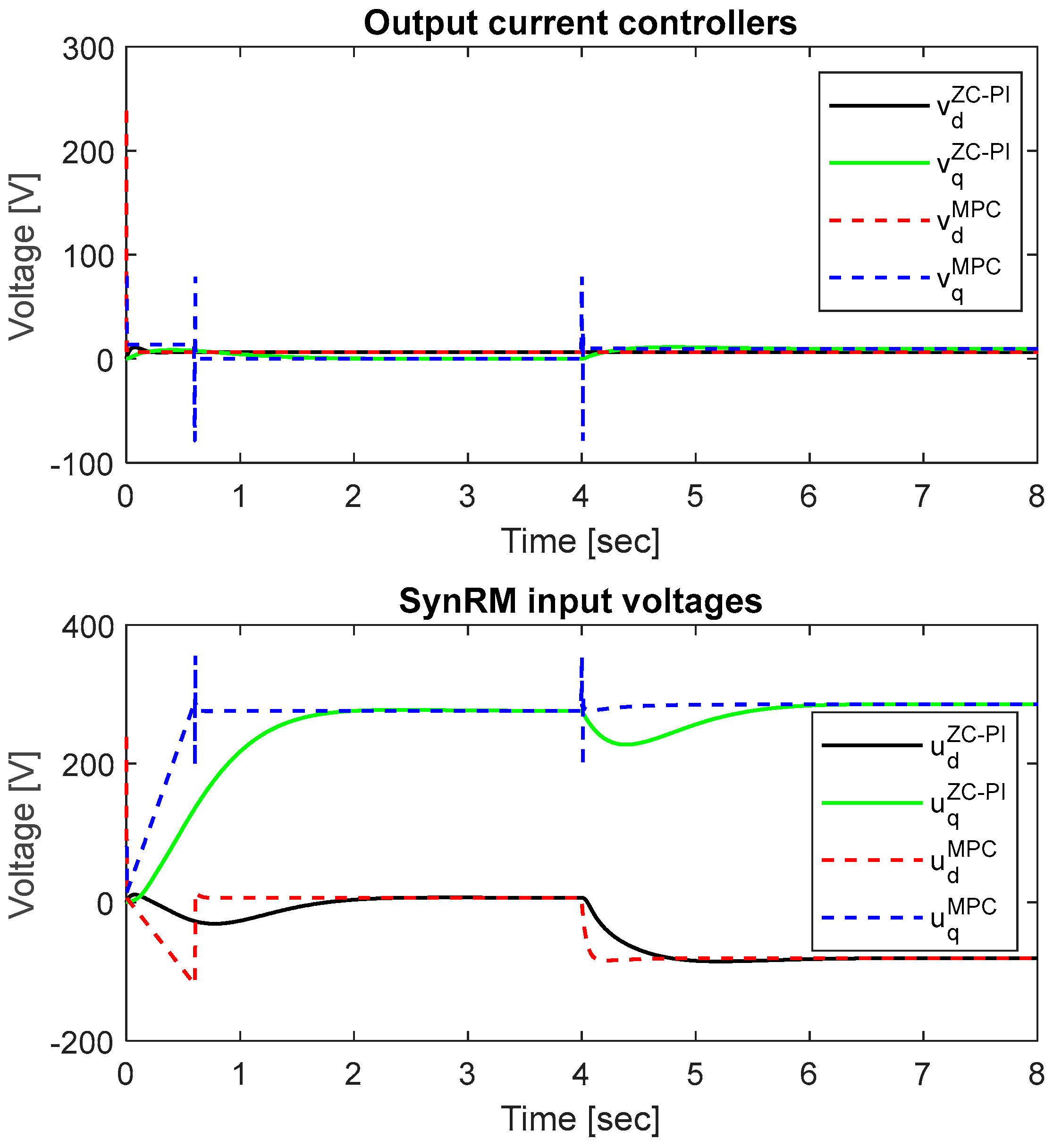
The output current controllers and the input voltages of SynRM dq model are illustrated in Figure 7.
The MPCd/q controller outputs are limited by the adopted constraints from Table 2. However, in comparison with the ZC-PI controller outputs , the MPC controller outputs present high variation components that are limited by the imposed constraints. Taking into account (23-24), the input voltages of SynRM dq model and depend on the controller outputs and , and on current limitations via the feedforward decoupling voltages. Therefore, by current controller outputs constraints, the input voltages of SynRM dq model are limited.
Figure 7.
The output of the current controllers and the input voltages of SynRM dq model.
Finally, it can be concluded that the MPC algorithms with related constraints used in the FOC cascade control structure improve the dynamic performances in comparison with the classical PI control.
5. Conclusions
The cascade MPC control structure based on FOC in the rotor reference frame allows us to obtain a high performance SynRM drive. By using the feedforward decoupling technique, the multivariable inner current loop of the cascade structure is transformed into two monovariable non-interaction linear systems, and thus, the two currents are independently controlled. Since the control strategy based on keeping constant the current on the d-axis was chosen for the cascade predictive control structure, the electromagnetic torque depends only on the q-axis current component, and hence, a linear MPC outer loop controller is used.
The critical constraints imposed on the electrical variables whose upper limits on the magnitude correspond to a circular limit in the dq plane were transformed into linear constraints through polygonal approximations to reduce the computational effort.
The steady state angular speed error due to the unmeasured disturbance introduced by the load torque and modeling errors is eliminated by adding an integral action and a feedforward component on the angular speed reference computation.
The performance of the proposed cascade predictive control structure based on FOC in the dq rotor reference frame for SynRM was evaluated in a simulation study using MPC controllers versus PI ones, resulting better behaviors of the MPC algorithms.
Author Contributions
Conceptualization, M.C. and C.L.; methodology, C.L. (Corneliu Lazar); software, M.C. (Madalin Costin); validation, M.C., and C.L.; formal analysis, C.L.; investigation, C.L.; resources, M.C.; writing—original draft preparation, M.C.; writing—review and editing, C.L.; visualization, M.C.; supervision, C.L. All authors have read and agreed to the published version of the manuscript.
Funding
This research received no external funding.
Data Availability Statement
Data availability is not applicable to this article as the study did not report any data.
Conflicts of Interest
The authors declare no conflicts of interest.
References
- Heidari, H.; Rassõlkin, A.; Kallaste, A.; Vaimann, T.; Andriushchenko, E.; Belahcen, A.; Lukichev, D. V. A review of synchronous reluctance motor-drive advancements. Sustainability 2021, 13, 729. [Google Scholar] [CrossRef]
- Pellegrino, G.; Jahns, T.; Bianchi, N.; Soong, W.; Cupertino, F. The Rediscovery of Synchronous Reluctance and Ferrite Permanent Magnet Motors; Springer International Publishing: Berlin/Heidelberg, Germany, 2016. [Google Scholar]
- Sul, S.K. Control of Electric Machine Drive Systems; John Wiley and Sons: Hoboken, USA, 2011. [Google Scholar]
- Betz, R. E.; Lagerquist, R.; Jovanovic, M.; Miller, T. J. E.; and Middleton R., H. Control of synchronous reluctance machines. IEEE Trans. Ind. Appl. 1993, 29, 1110–1122. [Google Scholar] [CrossRef]
- Hadla, H. Predictive Load Angle and Stator Flux Control of SynRM Drives for the Full Speed Range. PhD Dissertation-Coimbra University, August 2018. 20 August.
- Toliyat, H. A.; Shi, R.; Xu, H. A. DSP-Based Vector Control of Five-Phase Synchronous Reluctance Motor. In Proceedings of the Conference Record of the 2000 IEEE Industry Applications Conference. Thirty-Fifth IAS Annual Meeting and World Conference on Industrial Applications of Electrical Energy, Rome, Italy, 8 - 12 October 2000; pp. 1759–1765. [Google Scholar]
- Farhan, A.; Abdelrahem, M.; Hackl, C.M.; Kennel, R.; Shaltout, A.; Saleh, A. Advanced strategy of speed predictive control for nonlinear synchronous reluctance motors. Machines 2020, 8, 44. [Google Scholar] [CrossRef]
- Farhan, A.; Abdelrahem, M.; Saleh, A.; Shaltout, A.; Kennel, R. Simplified sensorless current predictive control of synchronous reluctance motor using online parameter estimation. Energies 2020, 13, 492. [Google Scholar] [CrossRef]
- Hadla, H.; Santos, F. Performance comparison of field-oriented control, direct torque control, and model-predictive control for SynRMs. Chin. J. Electr. 2022, 8, 24–37. [Google Scholar] [CrossRef]
- Carlet, P.G.; Tinazzi, F.; Bolognani, S.; Zigliotto, M. An effective model-free predictive current control for synchronous reluctance motor drives. IEEE Trans. Ind. Appl. 2019, 55, 3781–3790. [Google Scholar] [CrossRef]
- Carlet, P.G.; Tinazzi, F.; Ortombina, L.; and Bianchi, N. Sensorless Motor Parameter-Free Predictive Current Control of Synchronous Reluctance Motor Drives. In Proceedings of the International Conference on Electrical Machines (ICEM), Valencia, Spain, 5-8 September 2022; pp. 1464–1470. [Google Scholar]
- De Martin, I. D.; Pasqualotto, D.; Tinazzi, F.; Zigliotto, M. Model-free predictive current control of synchronous reluctance motor drives for pump applications. Machines 2021, 9, 217. [Google Scholar] [CrossRef]
- Costin, M.; Lazar, C. Comparative Study of Predictive Current Control Structures for a Synchronous Reluctance Machine. In Proceedings of the 26th International Conference on System Theory, Control and Computing (ICSTCC), Sinaia, Romania, 19-21 October 2022; pp. 530–535. [Google Scholar]
- Liu, T.-H.; Ahmad, S.; Mubarok, M.S.; Chen, J.-Y. Simulation and implementation of predictive Speed controller and position observer for sensorless synchronous reluctance motors. Energies 2020, 13, 2712. [Google Scholar] [CrossRef]
- Geyer, T.; Papafotiou, G.; Morari, M. Model predictive direct torque control - part i: concept, algorithm, and analysis. IEEE Trans. Ind. Elect. 2009, 56, 1894–1905. [Google Scholar] [CrossRef]
- Cimini, G.; Bernardini, D.; Bemporad, A.; and Levijoki, S. Online Model Predictive Torque Control for Permanent Magnet Synchronous Motors, In Proceedings of the IEEE International Conference on Industrial Technology (ICIT), Seville, Spain, 17-19 March 2015.
- Zanelli, A.; Kullick, J.; Eldeeb, H.M.; Frison, G.; Hackl, C.M.; Diehl, M. Continuous control set nonlinear model predictive control of reluctance synchronous machines. IEEE Trans. Control. Syst. Technol. 2022, 30, 130–141. [Google Scholar] [CrossRef]
- Azizi Moghaddam, H.; Rezaei, O.; Vahedi, A; Saeidi, M.; Mohsen Ehsani, M. A continuous control set of the model predictive controller of PMA-SynRM machine for high-performance flywheel energy storage system. Int. J. Dyn. Control 2022, 10, 1553–1566. [CrossRef]
- Wang, L.; Chai S.; Yoo, D.; Gan, L.; and Ng, K. PID and Predictive Control of Electrical Drives and Power Converters, Wiley: New York, USA: Wiley, 2015.
- Hilairet, M.; Lubint, T.; Tounzi, A. Variable reluctance machines: modeling and control, in Control of Non-Conventional Synchronous Motors.; Editor Louis J.P.; Wiley: London-Hoboken, Great Britain and the United States, 2012, pp. 287-328.
- Bolognani, S.; Bolognani, S.; Peretti, L.; Zigliotto, M. Design and implementation of model predictive control for electrical motor drives. IEEE Trans. Ind. Electron. 2009, 56, 1925–1936. [Google Scholar] [CrossRef]
- Bemporad, A. Model Predictive Control Design: New Trends and Tools. In Proceedings of the 45th IEEE Conference on Decision & Control, San Diego,USA, 13-15 December, 2006, pp. 6678-6683.
- Bemporad, A.; Morari, M.; Ricker, N.L. Model predictive control toolbox for Matlab – user’s guide. The Mathworks, Inc. 2023. Available online: https://www.mathworks.com/help/pdf_doc/mpc/mpc_ug.pdf (accessed on 14 March 2023).
- Boldea, I.; Paicu, M. C.; Andreescu, G.-D. Active flux concept for motion sensorless unified AC drives. IEEE Trans. Power Electron. 2008, 5, 2612–2618. [Google Scholar] [CrossRef]
- Stulrajter, M.; Sustek. P. Motor control application tuning (MCAT) tool for 3-phase PMSM, Application note. Freescale Semiconductor.
- Åström, K. J.; Hägglund, T. PID Controllers: Theory, Design, and Tuning; ISA - The Instrumentation, Systems and Automation Society: North Carolina, USA, 1995. [Google Scholar]
- Hadla, H.; Cruz, S. Active Flux Based Finite Control Set Model Predictive Control of Synchronous Reluctance Motor Drives. In Proceedings of the 18th European Conference on Power Electronics and Applications (EPE'16 ECCE Europe), Karlsruhe, Germany, 5-9 September 2016. [Google Scholar]
Disclaimer/Publisher’s Note: The statements, opinions and data contained in all publications are solely those of the individual author(s) and contributor(s) and not of MDPI and/or the editor(s). MDPI and/or the editor(s) disclaim responsibility for any injury to people or property resulting from any ideas, methods, instructions or products referred to in the content. |
© 2023 by the authors. Licensee MDPI, Basel, Switzerland. This article is an open access article distributed under the terms and conditions of the Creative Commons Attribution (CC BY) license (http://creativecommons.org/licenses/by/4.0/).
Copyright: This open access article is published under a Creative Commons CC BY 4.0 license, which permit the free download, distribution, and reuse, provided that the author and preprint are cited in any reuse.


