Submitted:
12 May 2023
Posted:
12 May 2023
Read the latest preprint version here
Abstract
We develop a quantitative microscopic theory of decaying Turbulence by studying the dimensional reduction of the Navier-Stokes loop equation for the velocity circulation. We have found an infinite dimensional manifold of solutions of the Navier-Stokes loop equation\cite{M93, M23PR} for the Wilson loop in decaying Turbulence in arbitrary dimension $d >2$. This family of solutions corresponds to a fractal curve in complex space $\mathbb C^d$, described by an algebraic equation between consecutive positions. The probability measure is explicitly constructed in terms of products of conventional measures for orthogonal group $SO(d)$ and a sphere $\mathbb S^{d-3}$. In three dimensions $d=3$, we compute a fractal dimension $d_f = 1.07$ for this fractal curve and the step size CDF with fat tail $x^{-2.15} $. We also compute the enstrophy CDF with fat tail $x^{-0.951}$, corresponding to an infinite mean value (anomalous dissipation). The energy density of the fluid decays as $\mathcal E_0/t$, where $\mathcal E_0$ is an initial dissipation rate. Presumably, we have found a new phase of extreme Turbulence not yet observed in real or numerical experiments.
Keywords:
Turbulence
; Fractal
; Anomalous dissipation
; Fixed point
; Velocity circulation
; Loop Equations
1. Introduction
A while ago, we derived [1,3] a functional equation for the so-called loop average [4,5] or Wilson loop in Turbulence. The path to an exact solution by a dimensional reduction in this equation was proposed in the ’93 paper [1], but we have only started exploring this path.
At the time, we could not compare a theory with anything but crude measurements in physical and numerical experiments at modest Reynolds numbers. All these experiments agreed with the K41 scaling, so the exotic equation based on unjustified methods of quantum field theory was premature.
The specific prediction of the Loop equation, namely the Area law [1], could not be verified in DNS at the time with existing computer power.
The situation has changed over the last decades. No alternative microscopic theory based on the Navier-Stokes equation emerged, but our understanding of the strong turbulence phenomena grew significantly.
On the other hand, the loop equations technology in the gauge theory also advanced over the last decades. The correspondence between the loop space functionals and the original vector fields was better understood, and various solutions to the gauge loop equations were found.
In particular, the momentum loop equation was developed, similar to our momentum loop used below [6,7,8]. Recently, some numerical methods were found to solve loop equations beyond perturbation theory [9,10].
The loop dynamics was extended to quantum gravity, where it was used to study nonperturbative phenomena [11,12].
All these old and new developments made loop equations a major nonperturbative approach to gauge field theory.
So, it is time to revive the hibernating theory of the loop equations in Turbulence, where these equations are much simpler.
The latest DNS [13,14,15,16] with Reynolds numbers of tens of thousands revealed and quantified violations of the K41 scaling laws. These numerical experiments are in agreement with so-called multifractal scaling laws [17].
However, as we argued in [2,18], at those Reynolds numbers, the DNS cannot yet distinguish between pure scaling laws with anomalous dimension and some algebraic function of the logarithm of scale modifying the K41 scaling.
Theoretically, we studied the loop equation in the confinement region (large circulation over large loop C), and we have justified the Area law, suggested back in ’93 on heuristic arguments [1].
This law says that the PDF tails of velocity circulation PDF in the confinement region are functions of the minimal area inside this loop.
It was verified in DNS four years ago [13] which triggered the further development of the geometric theory of turbulence[2,14,15,16,18,19,20,21,22,23,24,25,26,27,28,29,30].
In particular, the Area law was justified for flat and quadratic minimal surfaces [22], and an exact scaling law in confinement region was derived [21]. The area law was verified with better precision in [14].
It was later conjectured in [18] that the dominant field configurations in extreme Turbulence are so-called Kelvinons, which were shown to solve stationary Navier-Stokes equations assuming the sparse distribution of vorticity structures.
These topological solitons of the Euler theory are built around a vortex sheet bounded by a singular vortex line. This vortex line is locally equivalent to the cylindrical Burgers vortex [31], with infinitesimal thickness in the limit of a large Reynolds number.
As we argued in [2,18], the Kelvinon has an anomalous dissipation, surviving the strong turbulent limit. This dissipation is proportional to the square of constant circulation of the Burgers vortex times a line integral of the tangent component of the strain along the loop.
The Kelvinon minimizes the energy functional, with anomalous terms coming from the Burgers core of the vortex line. There is also a constant scale factor Z in the representation of the Kelvinon vorticity in terms of spherical Clebsch variables:
In that paper, the constant Z was related to the Kolmogorov energy dissipation density and the boundary value of the variable at the loop C.
The anomalous Hamiltonian [2,18] explicitly violated the K41 scaling by the logarithmic terms in the region of small loops C. This region resembles the asymptotically free QCD. The logarithmic terms were summed up by RG equation with running coupling constant logarithmically small in this region.
These exciting developments explain and quantitatively describe many interesting phenomena [2] but do not provide a complete microscopic theory covering the full inertial range of Turbulence without simplifying assumptions of the sparsity of vortex structures.
Moreover, while the Kelvinon (presumably) solves the stationary Navier-Stokes equations, it does not solve the loop equations for the following reason.
The loop equation assumes that the velocity field is independent of the loop C. In this case, the variations of the circulation in the loop functional with respect to the shape C of the loop can be reduced to the Navier-Stokes equation.
Otherwise, the variation would also involve the variation of the velocity field .
This problem does not invalidate the Kelvinon theory as an ideal gas of random vortex rings sparsely distributed in a turbulent flow.
The loop functional is not needed for that statistical theory, and the stationary solution of the Navier-Stokes equation is sufficient. The shape of the loop and the vortex sheet inside would become random variables influenced by a background strain like in the pure vortex sheet solutions [2].
These objections, however, prevent the Kelvinon gas model from being a complete theory of strong isotropic Turbulence. This is merely an approximation of the full theory.
In the present work, we develop the theory free of these assumptions by exactly solving the loop equations for decaying turbulence. Our representation of velocity circulation does not run into the problems of the Kelvinon gas model; nor do we make any approximations in the loop equations we are solving.
2. Loop Equation
We introduced the loop equation in Lecture Series at Cargese and Chernogolovka Summer Schools [1].
Here is a summary for the new generation.
We write the Navier-Stokes equation as follows
The Wilson loop average for the Turbulence
treated as a function of time and a functional of the periodic function (not necessarily a single closed loop), satisfies the following functional equation
The statistical averaging corresponds to initial randomized data, to be specified later.
The area derivative is related to the variation of the functional when the little closed loop is added
In the review, [1,2], we present the explicit limiting procedure needed to define these functional derivatives in terms of finite variations of the loop while keeping it closed.
All the operators are expressed in terms of the spike operator
The area derivative operator can be regularized as
and velocity operator (with )
In the Navier-Stokes equation, we did NOT add customary Gaussian random forces, choosing instead to randomize the initial data for the velocity field.
These random forces would lead to the potential term [2] in the loop Hamiltonian , breaking certain symmetries needed for the dimensional reduction we study below.
With random initial data instead of time-dependent delta-correlated random forcing, we no longer describe the steady state (i.e., statistical equilibrium) but decaying Turbulence, which is also an interesting process, manifesting the same critical phenomena.
The energy is pumped in at the initial moment and slowly dissipates over time, provided the viscosity is small enough, corresponding to the large Reynolds number we are studying.
3. Dimensional Reduction
The crucial observation in [1] was that the right side of the Loop equation, without random forcing, dramatically simplifies in functional Fourier space. The dynamics of the loop field can be reproduced in a simple Ansatz
The difference with the original definition of is that our new function depends directly on rather then through the function taken at .
This transformation is the dimensional reduction we mentioned above. From the point of view of the loop functional, there is no need to deal with field ; one could take a shortcut.
The reduced dynamics must be fitted to the Navier-Stokes dynamics of the original field. With the loop calculus developed above, we have all the necessary tools to build these reduced dynamics.
Let us stress an important point: the function is independent of the loop C. As we shall see later, it is a random variable with a universal distribution in functional space.
This removes an objection we made in the Introduction to the Kelvinon theory as well as any other Navier-Stokes stationary solutions, with a singularity at fixed loop C in space.
The functional derivative, acting on the exponential in (13) could be replaced by the derivative as follows
The equation for as a function of and also a function of time, reads:
where the operators should be regarded as ordinary numbers, with the following definitions.
This transformation yields the following formula for the spike derivative D in the above equation
The vorticity operator (11) and velocity (12) become ordinary numbers, which are some singular functionals of the trajectory .
The first observation about this equation is that the viscosity factor cancels after the substitution (16).
As we shall see, the viscosity enters initial data so that at any finite time t, the solution for P still depends on viscosity.
Another observation is that the spike derivative turns to the discontinuity in the limit
The relation of the operators in the QCD loop equation to the discontinuities of the momentum loop was noticed, justified, and investigated in [7,8].
In the Navier-Stokes theory, this relation provides the key to the exact solution.
In the same way, we find the limit for vorticity
and velocity (skipping the common argument )
We arrive at a singular equation
This equation is complex due to the irreversible dissipation effects in the Navier-Stokes equation.
The viscosity dropped from the right side of this equation; it can be absorbed in units of time. Viscosity also enters the initial data, as we shall see in the next section on the example of the random rotation.
However, the large-time asymptotic behavior of the solution would be universal, as it should be in the Turbulent flow.
We are looking for a degenerate fixed point [2], a fixed manifold with some internal degrees of freedom. The spontaneous stochastization corresponds to random values of these hidden internal parameters.
Starting with different initial data, the trajectory would approach this fixed manifold at some arbitrary point and then keep moving around it, covering it with some probability measure.
The Turbulence problem is to find this manifold and determine this probability measure.
4. Random Global Rotation
Possible initial data for the reduced dynamics were suggested in the original papers [1,2]. The simplest but still meaningful distribution of the initial velocity field is the Gaussian one, with energy concentrated in the macroscopic motions. The corresponding loop field reads
where is the velocity correlation function
The potential part drops out in the closed loop integral.
The correlation function varies at the macroscopic scale, which means that we could expand it in the Taylor series
The first term is proportional to initial energy density,
and the second one is proportional to initial energy dissipation rate
where is the dimension of space.
The constant term in (25) as well as terms drop from the closed loop integral, so we are left with the cross-term , which reduces to a full square
This distribution is almost Gaussian: it reduces to Gaussian one by extra integration
The integration here involves all independent components of the antisymmetric tensor . Note that this is ordinary integration, not the functional one.
The physical meaning of this is the random uniform vorticity at the initial moment.
Unfortunately, as we see it now, this initial data represents a spurious fixed point unrelated to the turbulence problem.
It was discussed in our review paper [2]. The uniform global rotation represents a fixed point of the Navier-Stokes equation for arbitrary uniform vorticity tensor.
Gaussian integration by keeps it as a fixed point of the Loop equation.
The time derivative at this special initial data vanishes so that the exact solution of the loop equation with this initial data equals its initial value (28).
Naturally, the time derivative of the momentum loop with the corresponding initial data will vanish as well.
It is instructive to look at the momentum trajectory for this fixed point.
The functional Fourier transform [1,2] leads to the following simple result for the initial values of .
In terms of Fourier harmonics, this initial data read
As for the constant part of , it is not defined, but it drops from equations by translational invariance.
Note that this initial data is not real, as . Positive and negative harmonics are real but unequal, leading to a complex Fourier transform. At fixed tensor the correlations are
5. Decay or Fixed Point
The absolute value of loop average stays below 1 at any time, which leaves two possible scenarios for its behavior at a large time.
The Decay scenario in the nonlinear ODE (22) corresponds to the decrease of .
Omitting the common argument , we get the following exact time-dependent solution (not just asymptotically, at ).
The Fixed Point would correspond to the vanishing right side of the momentum loop equation (22). Multiplying by and reducing the terms, we find a singular algebraic equation
The fixed point could mean self-sustained Turbulence, which would be too good to be true, violating the second law of Thermodynamics. Indeed, it is easy to see that this fixed point cannot exist.
The fixed point equation (41) is a linear relation between two vectors with coefficients depending on various scalar products. The generic solution is simply
with the complex parameter to be determined from the equation (41).
This solution is degenerate: the fixed point equation is satisfied for arbitrary complex .
The discontinuity vector aligned with the principal value corresponds to vanishing vorticity in (18), leading to a trivial solution of the loop equation .
We are left with the decaying turbulence scenario (39) as the only remaining physical solution.
6. Random Walk in Complex space
One may try the solution where the discontinuity vector is proportional to the principal value. However, in this case, such a solution does not exist.
There is, however, another solution where the vectors are not aligned. This solution requires the following relations
These relations are interesting. The complex numbers indicate irreversibility and lack of alignment leads to vorticity distributed along the loop.
Also, note that this complex vector is dimensionless, and the fixed point equation (Section 6) is completely universal!
One can iteratively build this solution as a fractal curve by the following method.
Start with a complex vector .
We compute the next values from the following discrete version of the discontinuity equations (Section 6).
The solution of these equations can be represented using a complex vector subject to two complex constraints
after which we can find the next value
We assume N steps, each with the angle shift .
Note that the complex unit vector is not defined with the Euclidean metric in six dimensions . Instead, we have a complex condition
which leads to two conditions between real and imaginary parts
In d dimensions, there are complex parameters of the unit vector; with an extra linear constraint in (47), there are now free complex parameters at every step of our iteration, plus the discrete choice of the sign of the root in the solution of the quadratic equation.
At the last step, , we need to get a closed loop . This is one more constraint on the complex vectors
We use this complex vector constraint to fix the arbitrary initial complex vector as a function of all remaining parameters.
We have here a nonlinear random walk in complex vector space . The complex unit step depends on the current position .
The initial position is adjusted to close the trajectory after N steps at given rotations.
We are interested in the limit of infinitely many steps , corresponding to a closed fractal curve with a discontinuity at every point.
7. The Probability measure
The simplest case where these equations have nontrivial solutions is in three-dimensional space. For smaller dimensions, there is only a degenerate solution with zero vorticity (a vanishing cross product ).
The complex unit vector in d dimensions can be parametrized by rotation matrix and a unit real vector in dimensions
The complex constraint for can be used to fix these as a linear function of given a complex vector
as follows:
where and
After that, yields a quadratic equation for .
Note in passing that belongs to De Sitter space . However, this is where an analogy with the ADS/CFT duality ends.
There are, in general, four solutions for : two signs for R in () and two more signs in a solution of the quadratic equation for (53a). We have to choose one of these four solutions at each step, also selecting the real solution for .
The simple universal choice, which works in numerical simulations, is the solution with the smallest Euclidean length .
The motivation for this minimization is that there is no upper limit on the solution for . The unminimized random walk may rapidly go to infinity due to instabilities.
With this minimization restriction, the step size s distribution we find below in numerical simulation decays as , sufficient for finite mean and variance.
We also found that the mean Euclidean distance of unconstrained random walk grows approximately linearly with the number N of steps, not showing any sign of instabilities.
We conclude that the fixed manifold of the decaying Turbulence is a tensor product of spaces
We arrive at the invariant distribution for our fractal curve. At a fixed number of steps, N
where are complex vectors, parametrized by via recurrent equations (Section 7),(55).
The complex vector’s integration and delta function is understood as a product of its real and imaginary parts. This integration leads to a Jacobian factor in the measure, depending on the relative angles between all rotations.
This closure condition is sufficient by parameter count to eliminate a complex vector ; however, doing this at an arbitrary number of rotation matrices is a nontrivial technical problem.
We will address this and other technical problems in three dimensions using Mathematica®.
The remarkable universality of this fractal curve in complex space makes these problems worth an effort.
As for the computation of the Jacobian in (60), it is easier than it looks.
There is a recurrent equation (in matrix notations, with complex vector treated as 6 dimensional real vector)
Finally, using the chain rule, we compute the Jacobian (the orthogonal matrices all cancel)
8. Reflected solution and Wilson loop convergence
There is an obvious problem with the solution we have found. The loop equation for is complex, and so is the solution, particularly the vorticity in (18). Since the equation for is nonlinear, we cannot add a complex conjugate solution. Besides, the complex conjugate solution would not satisfy the same nonlinear equation (Section 6) with complex coefficients.
As we shall see later, the distribution of the random variables decays only as a power. This makes the exponential in the Wilson loop grow too fast for the power distribution to converge.
However, another solution corresponds to solving the recurrent equations (Section 6) in the opposite direction on the loop. In the continuum limit, it corresponds to the orientation reversal .
A discrete version corresponds to counting points in the opposite direction on a loop. In the equations (Section 6), only the sign in front of the gap will change, equivalent to a complex conjugation of the equation. In other words, the solution with the opposite orientation is the complex conjugate of the original solution .
One of these two solutions would correspond to the exponential growth of the Wilson loop, and another one - to exponential decrease
The increment of exponential growth/decrease generally depends on the loop C.
We conclude that only one of these two solutions is acceptable in various regions of the loop space C.
Another problem is that we expect the correlation functions of vorticity (see the next section) to be real. Presumably, the ambiguities of the probability measure can be used to cancel imaginary parts of observable expectation values.
This issue remains unsolved and requires further investigation.
9. Vorticity Distribution and Energy dissipation
The simplest quantity to compute in our theory is the local vorticity distribution.
As we shall see, it determines the energy dissipation rate.
The local vorticity for our decaying solution of the loop equation
Here is an arbitrary point at the loop, which makes this expression a random variable.
Note that viscosity is canceled here, as it should be by dimensional counting (vorticity has the dimension of ).
In our random walk representation, the complex vorticity operator
The time derivative of energy density in our theory is
Solving this equation with boundary value we relate to mean initial energy
The probability distribution of and its mean value can be computed using our random walk. For the anomalous dissipation, we need the mean enstrophy to diverge [2,18] , so that viscosity is compensated in the extreme turbulent limit.
As we shall see later, in Section 11, this is what happens in our numerical simulations.
The microscopic picture of this infinite enstrophy differs from the singular vortex line.
In the Euler theory, divergence came from the singularity of the classical field. However, in our dual theory, it comes from the large fluctuation of the fractal curve in momentum space.
We can now write down our result for the Wilson loop in decaying Turbulence as a functional of the contour C. Let us start with a three-dimensional case
The finite steps approximation we considered above
For the simplest circular loop in an plane, we have
We observe that even at the large time when the asymptotic fractal curve is already in place, there is a region of parameters
where the Wilson loop is a nontrivial universal function of a single variable
We can compute our prediction for this function by numerically solving the recurrent equations for our vectors and wait for the results with physical or numerical experiments in conventional three-dimensional decaying Turbulence.
10. Correlation Functions
The simplest observable quantities we can extract from the loop functional are the vorticity correlation functions [2], corresponding to the loop C backtracking between two points in space , see Figure 1. The vorticity operators are inserted at these two points.
The correlation function reduces to a random walk with a complex weight
In Fourier space, this reduces to the restricted random walk:
The numerical simulation of this correlation function would require significant computer resources.
Still, these resources are much more modest than those for full d dimensional simulations of the Navier-Stokes equation.
In our theory, the dimension of space enters as the number of components of the one-dimensional fluctuating field rather than the number of variables in the fluctuating velocity field .
Also, note that our quantum problem of the complex random walk naturally fits quantum computer architecture. Thus, in the future, when large quantum computers would become available for researchers, we can expect a real breakthrough in numerical simulations of the loop equation.
11. Computations
We wrote a Mathematica® program [32] generating our random walk, starting with a random complex vector and using random orthogonal matrix at every step.
For 1000 steps, it takes a few seconds on a laptop to compute the whole path.
The closure of the path requires special efforts. We create a frozen set of random orthogonal matrices for the path with N steps.
At each step we use the frozen random matrix and choose from four solutions for the one closest to the initial point by Euclidean distance in six dimensions .
Then we generate a parallel table of 10000 paths with various random initial vectors .
We use a Monte-Carlo minimization of the absolute distance between initial and final vectors . Altogether, it took steps of a random walk.
The convergence to zero of the sequence of these absolute distances is shown in Figure 2 in logarithmic scale.
The simplest quantity to compute is a fractal dimension of this random walk, defined as
The ordinary Brownian motion (linear random walk) has , but our random walk is very different, mainly because the Euclidean distance of an elementary step in De Sitter space is unlimited from above (though it is limited by 1 from below).
Here is the plot of vs (Figure 4).
The statistical data for parameters
This data is compatible with .
The distribution of the Euclidean length of each step (Figure 5).
The statistical table for the parameters of this fit
The mean value and error of a step is
Another interesting distribution is in (69).
The CDF is shown in Figure 6. The tail is compatible with decay, corresponding to the decay of the PDF. The mean value and all higher moments diverge, leading to anomalous dissipation.
The statistical table for the parameters of this fit
The computation of the Wilson loop and related correlation functions of vorticity needs an ensemble of closed fractal loops with various sets of random matrices.
The closure condition for the loop would require some computational effort because the probability of the random curve with fractal dimension returning to an initial point goes to zero with the increased number of steps.
An alternative approach of starting with a large closed loop and randomizing it point by point while preserving its closure.
These extra layers of computational complexity would require a supercomputer, which we plan to do later.
12. Discussion
We have presented an exact solution of the Navier-Stokes loop equations for the Wilson loop in decaying Turbulence as a functional of the shape and size of the loop in arbitrary dimension .
An expert in the conventional theory of Turbulence may wonder why the solutions of the Loop equation are relevant to the statistical distribution of the vorticity in a decaying turbulent flow.
Such questions were asked and answered in the gauge theories, including QCD[6,8,9,10] where the loop equations were derived first [4,5].
The solution of the loop equation with finite area derivative belongs to the so-called Stokes-type functionals [4], the same as the Wilson loop for Gauge theory and fluid dynamics.
Extra complications in the gauge theory, which are fortunately absent in fluid dynamics, are the short-distance singularities related to the infinite number of fluctuating degrees of freedom in quantum field theory.
As we discussed in detail in [2,4,5], any Stokes-type functional satisfying boundary condition at shrunk loop , and solving the loop equation can be iterated in the nonlinear term in the Navier-Stokes equations (which applies at large viscosity).
The resulting expansion in inverse powers of viscosity (weak Turbulence) exactly coincides with the ordinary perturbation expansion described by Wylde diagrams.
As we have seen, the Anzatz (13) satisfies the loop equation and initial condition at . It has a finite area derivative, which makes it a Stokes-type functional.
Moreover, we have shown in [1,2] (and also here, in Section 4) how the velocity distribution for the random uniform vorticity in the fluid was reproduced by our Anzatz (13) a singular momentum loop .
The solution for was random complex and had slowly decreasing Fourier coefficients, leading to a discontinuity in a pair correlation function (35).
The exact solution for in decaying Turbulence which we have found in this paper, also belongs to the Stokes functionals and satisfies the initial boundary value at the shrunk loop.
Therefore, it represents a statistical distribution in some Navier-Stokes flow, a degenerate fixed point of the Hopf equation for velocity circulation, summing up all the Wylde diagrams plus nonperturbative effects. Whether this exact solution is realized in Nature remains to be seen.
It is infinitely more complex than the randomly rotated fluid, as our curve has a discontinuity at every , corresponding to a distributed random vorticity.
This solution is described by a fractal curve in complex d dimensional space, a limit of a random walk with nonlinear algebraic relations between the previous position and the next one . These relations are degenerate: each step is characterized by an arbitrary element and an arbitrary element . This step also depends upon the previous position .
The periodicity condition provides a nonlinear equation for an initial position as a function of the above free parameters .
We simulated this random walk in three dimensions and studied its statistical properties. The fractal dimension of the random walk without the closure condition approximately equals . The distribution of lengths of steps in Euclidean six-dimensional space has a nontrivial power-like tail .
As for the distribution of an enstrophy density, it has a power tail corresponding to an infinite mean value and all higher moments. This infinity is how anomalous dissipation manifests in our solution.
There are many things to do next with this conjectured solution to the decaying turbulence problem; the first is to look for unnoticed inconsistencies.
As a first test of this solution, let us compare it with a multitude of experimental data and those from DNS [33].
There is no agreement between these data, they vary in Reynolds number, and they have other differences related to the experimental setup. No value n for the decay power would fit all that data. However, a consensus seems to be around , which means faster decay than we have.
We are skeptical about these data. As we recently learned [34], there is a regime change at large Reynolds numbers; the numbers achievable in modern DNS are at such a transitional regime.
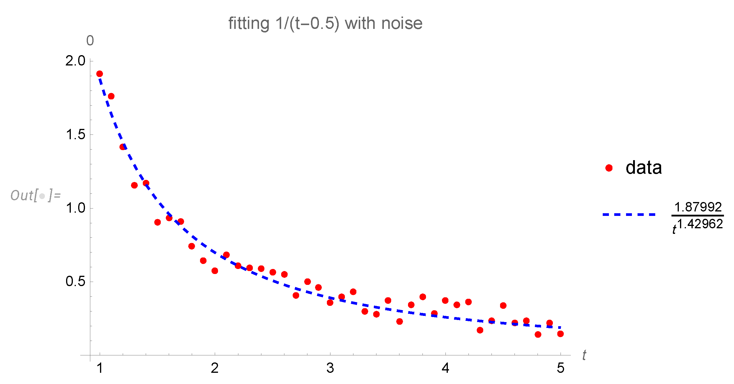
Besides, fitting is an unreliable method of deriving physical laws.
For example, we took a formula , added random noise between and fitted this data to . The best fit produced some fake power and some fake coefficient in front (see Figure 7).
Instead, one should compare a theory with a null hypothesis and estimate the probability of this null hypothesis to be correct.
Presumably, our fixed point corresponds to a true infinite Reynolds limit, as it is completely universal and does not depend on the Reynolds scales.
If you assume no hidden scales are left, our law follows from dimensional analysis. Observed or simulated data with all have the powers of some other dimensional parameters related to the Reynolds number. They rely on (multifractal versions of) K41 spectra and other intermediate turbulent phenomena.
We have an anomalous dissipation rate: the mean value of the vorticity square diverges, compensating for the viscosity factor in the energy decay in extreme turbulent limit.
This mechanism of anomalous dissipation differs from the one we studied in the Kelvinon [2,18]. In those fixed points, the viscosity canceled in the dissipation rate due to the singular vorticity configurations with the thin vortex line resolved as a core of a Burgers vortex. Here, in the dual theory of fractal momentum loop, the large fluctuations of this momentum loop lead to the divergent expectation value of the enstrophy.
Our solution is universal, rotational, and translational invariant. It has the expected properties of extreme isotropic Turbulence. Is it THE solution? Time will tell.
Data Availability Statement
We generated new data for the nonlinear complex random walk and the Wilson loop using the Mathematica® code. This code, the data, and the three-dimensional plots are publicly available in Wolfram Cloud [32].
Acknowledgments
I benefited from discussions of this theory with Sasha Polyakov, K.R. Sreenivasan, Greg Eyink, Luca Moriconi, Vladimir Kazakov, and Kartik Iyer. This research was supported by a Simons Foundation award ID 686282 at NYU Abu Dhabi.
References
- Migdal, A. Loop Equation and Area Law in Turbulence. In Quantum Field Theory and String Theory; Baulieu, L., Dotsenko, V., Kazakov, V., Windey, P., Eds.; Springer US, 1995; pp. 193–231. [Google Scholar] [CrossRef]
- Migdal, A. Statistical Equilibrium of Circulating Fluids. Physics Reports 2023, arXiv:physics.flu-dyn/2209.12312]1011C, 1–117. [Google Scholar] [CrossRef]
- Migdal, A.A. Random Surfaces and Turbulence. International Workshop on Plasma Theory and Nonlinear and Turbulent Processes in Physics, Kiev, April 1987; Bar’yakhtar, V.G., Ed.; World Scientific, 1988; p. 460. [Google Scholar]
- Makeenko, Y.; Migdal, A. Exact equation for the loop average in multicolor QCD. Physics Letters B 1979, 88, 135–137. [Google Scholar] [CrossRef]
- Migdal, A. Loop equations and 1N expansion. Physics Reports 1983, 201. [Google Scholar] [CrossRef]
- Migdal, A. Momentum loop dynamics and random surfaces in QCD. Nuclear Physics B 1986, 265, 594–614. [Google Scholar] [CrossRef]
- Migdal, A. Second quantization of the Wilson loop. Nuclear Physics B - Proceedings Supplements 1995, 41, 151–183. [Google Scholar] [CrossRef]
- Migdal, A.A. Hidden symmetries of large N QCD. Prog. Theor. Phys. Suppl. 1998, 131, 269–307. [Google Scholar] [CrossRef]
- Anderson, P.D.; Kruczenski, M. Loop equations and bootstrap methods in the lattice. Nuclear Physics B 2017, 921, 702–726. [Google Scholar] [CrossRef]
- Kazakov, V.; Zheng, Z. Bootstrap for lattice Yang-Mills theory. Phys. Rev. D 2023, arXiv:hep-th/2203.11360]107, L051501. [Google Scholar] [CrossRef]
- Ashtekar, A. New variables for classical and quantum gravity. Physical Review Letters 1986, 57, 2244–2247. [Google Scholar] [CrossRef]
- Rovelli, C.; Smolin, L. Knot Theory and Quantum Gravity. Phys. Rev. Lett. 1988, 61, 1155–1158. [Google Scholar] [CrossRef]
- Iyer, K.P.; Sreenivasan, K.R.; Yeung, P.K. Circulation in High Reynolds Number Isotropic Turbulence is a Bifractal. Phys. Rev. X 2019, 9, 041006. [Google Scholar] [CrossRef]
- Iyer, K.P.; Bharadwaj, S.S.; Sreenivasan, K.R. The area rule for circulation in three-dimensional turbulence. Proceedings of the National Academy of Sciences of the United States of America 2021, 118, e2114679118. [Google Scholar] [CrossRef] [PubMed]
- Apolinario, G.; Moriconi, L.; Pereira, R.; valadão, V. Vortex Gas Modeling of Turbulent Circulation Statistics. PHYSICAL REVIEW E 2020, 102, 041102. [Google Scholar] [CrossRef] [PubMed]
- Müller, N.P.; Polanco, J.I.; Krstulovic, G. Intermittency of Velocity Circulation in Quantum Turbulence. Phys. Rev. X 2021, 11, 011053. [Google Scholar] [CrossRef]
- Parisi, G.; Frisch, U. On the singularity structure of fully developed turbulence Turbulence and Predictability. In Proceedings of the Geophysical Fluid Dynamics: Proc. Intl School of Physics E. Fermi; M Ghil, R.B.; Parisi, G., 1985, Eds. Amsterdam: North-Holland; pp. 84–88.
- Migdal, A. Topological Vortexes, Asymptotic Freedom, and Multifractals. MDPI Fractals and Fractional, Special Issue. 2023, arXiv:2212.13356. [Google Scholar]
- Migdal, A. Universal Area Law in Turbulence. 2019, arXiv:1903.08613. [Google Scholar]
- Migdal, A. Scaling Index α=12 In Turbulent Area Law. 2019, arXiv:1904.00900v2. [Google Scholar]
- Migdal, A. Exact Area Law for Planar Loops in Turbulence in Two and Three Dimensions. 2019, arXiv:1904.05245v2. [Google Scholar]
- Migdal, A. Analytic and Numerical Study of Navier-Stokes Loop Equation in Turbulence. 2019, arXiv:1908.01422v1. [Google Scholar]
- Migdal, A. Turbulence, String Theory and Ising Model. 2019, arXiv:1912.00276v3. [Google Scholar]
- Migdal, A. Towards Field Theory of Turbulence. 2020, arXiv:2005.01231. [Google Scholar]
- Migdal, A. Probability Distribution of Velocity Circulation in Three Dimensional Turbulence. 2020, arXiv:2006.12008. [Google Scholar]
- Migdal, A. Clebsch confinement and instantons in turbulence. International Journal of Modern Physics A 2020, arXiv:hep-th/2007.12468v7]35, 2030018. [Google Scholar] [CrossRef]
- Migdal, A. Asymmetric vortex sheet. Physics of Fluids 2021, 33, 035127. [Google Scholar] [CrossRef]
- Migdal, A. Vortex sheet turbulence as solvable string theory. International Journal of Modern Physics A 2021, 36, 2150062. [Google Scholar] [CrossRef]
- Migdal, A. Confined Vortex Surface and Irreversibility. 1. Properties of Exact solution. 2021, arXiv:physics.flu-dyn/2103.02065v10. [Google Scholar] [CrossRef]
- Migdal, A. Confined Vortex Surface and Irreversibility. 2. Hyperbolic Sheets and Turbulent statistics. 2021, arXiv:physics.flu-dyn/2105.12719. [Google Scholar] [CrossRef]
- Wikipedia. Burgers vortex. Available online: https://en.wikipedia.org/wiki/Burgers_vortex (accessed on 27 April 2022).
- Migdal, A. Complex Nonlinear Random Walk. https://www.wolframcloud.com/obj/sasha.migdal/Published/FQequation.nb, 2023. 2023. Available online: https://www.wolframcloud.com/obj/sasha.migdal/Published/FQequation.nb.
- Panickacheril John, J.; Donzis, D.A.; Sreenivasan, K.R. Laws of turbulence decay from direct numerical simulations. Philosophical Transactions of the Royal Society A: Mathematical, Physical and Engineering Sciences 2022, 380, 20210089. [Google Scholar] [CrossRef]
- Sreenivasan, K.R.; Yakhot, V. The saturation of exponents and the asymptotic fourth state of turbulence. 2022. [Google Scholar] [CrossRef]
Figure 1.
Backtracking wires corresponding to vorticity correlation function.
Figure 2.
The closure gaps in the Monte-Carlo minimization.
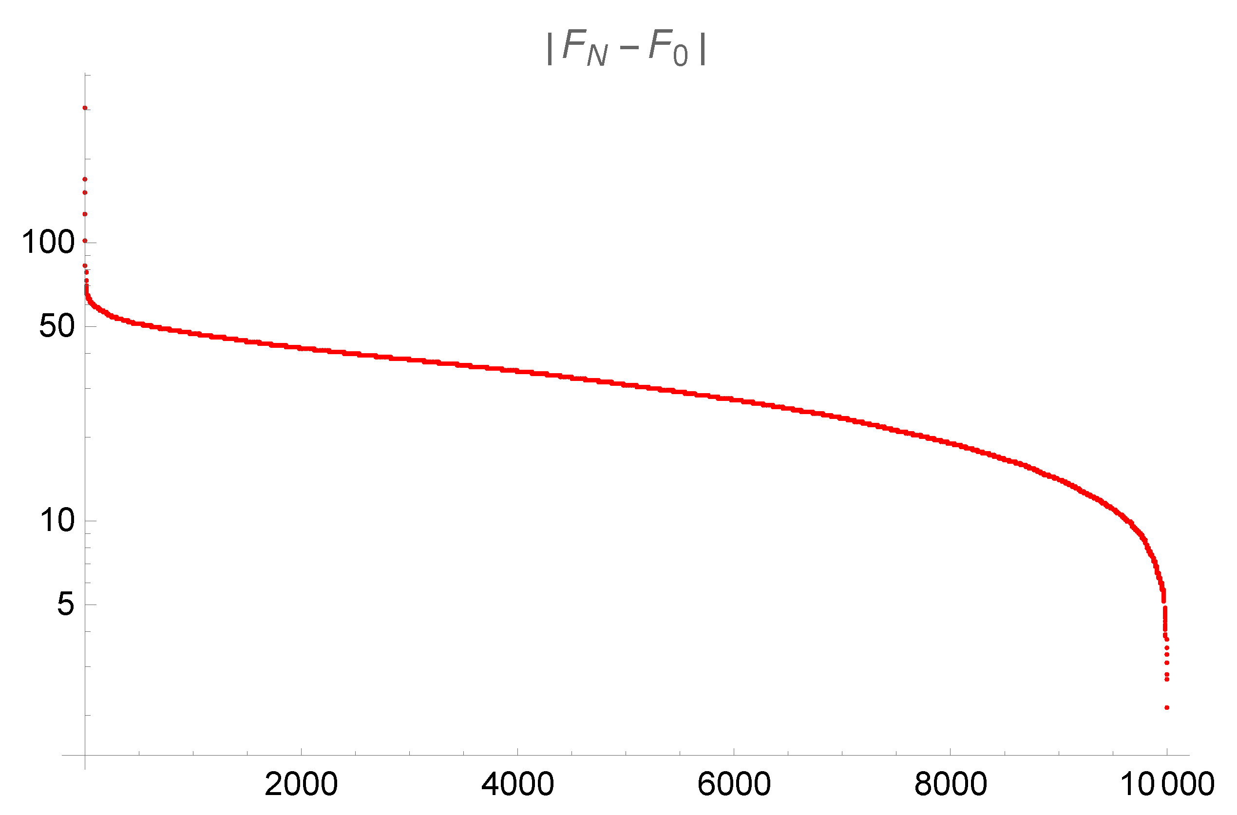
Figure 3.
A thousand steps of nonlinear random walk in complex three-dimensional space . The initial point is optimized to close the path after 1000 steps given a frozen set of 1000 random rotation matrices . Imaginary and real parts of the vector are displayed with different colors.
Figure 3.
A thousand steps of nonlinear random walk in complex three-dimensional space . The initial point is optimized to close the path after 1000 steps given a frozen set of 1000 random rotation matrices . Imaginary and real parts of the vector are displayed with different colors.
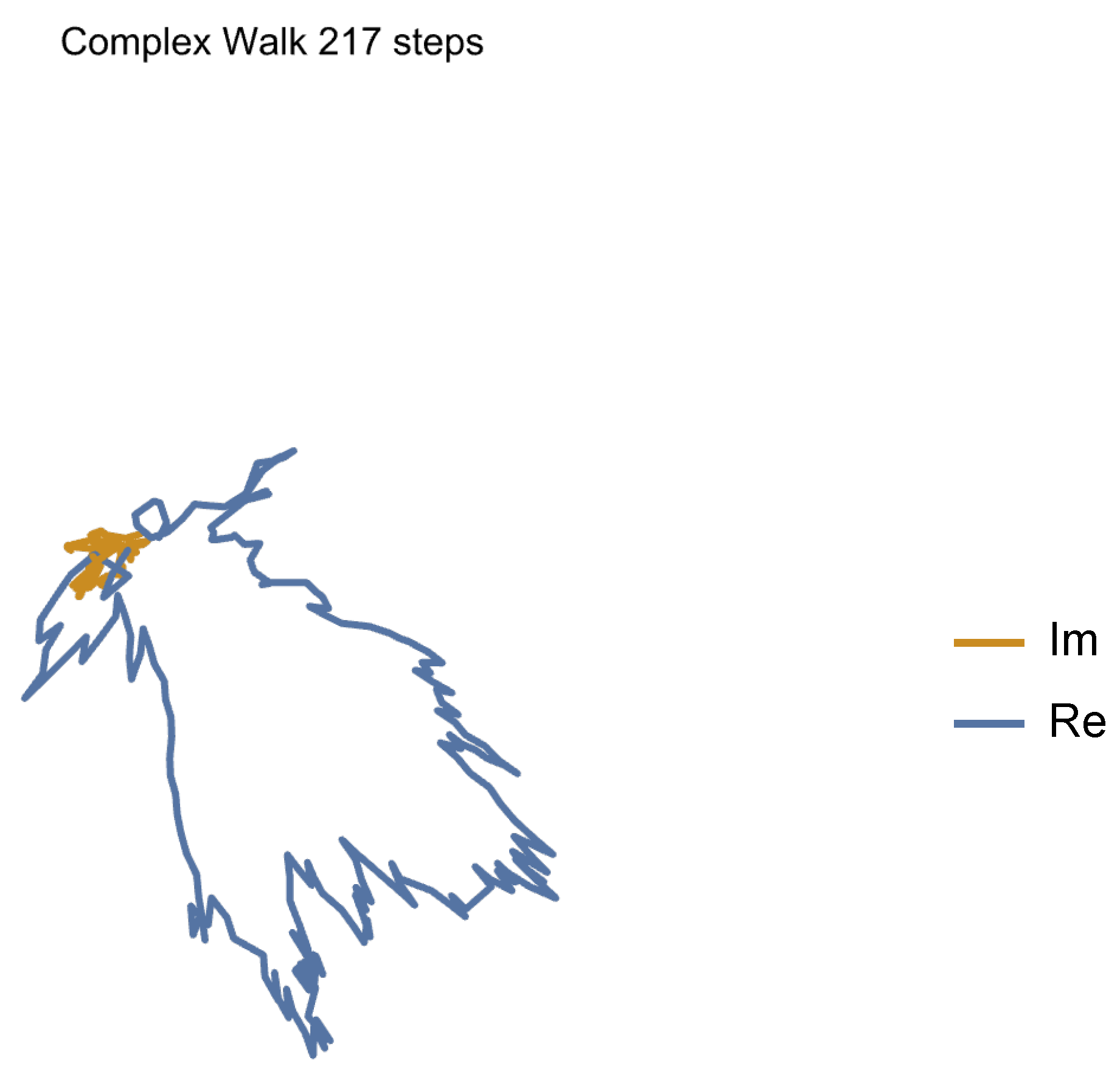
Figure 4.
Logarithm of Euclidean distance for our random walk in six-dimensional space as a function of a logarithm of the number of steps. The linear fit corresponds to fractal dimension , compatible with .
Figure 4.
Logarithm of Euclidean distance for our random walk in six-dimensional space as a function of a logarithm of the number of steps. The linear fit corresponds to fractal dimension , compatible with .
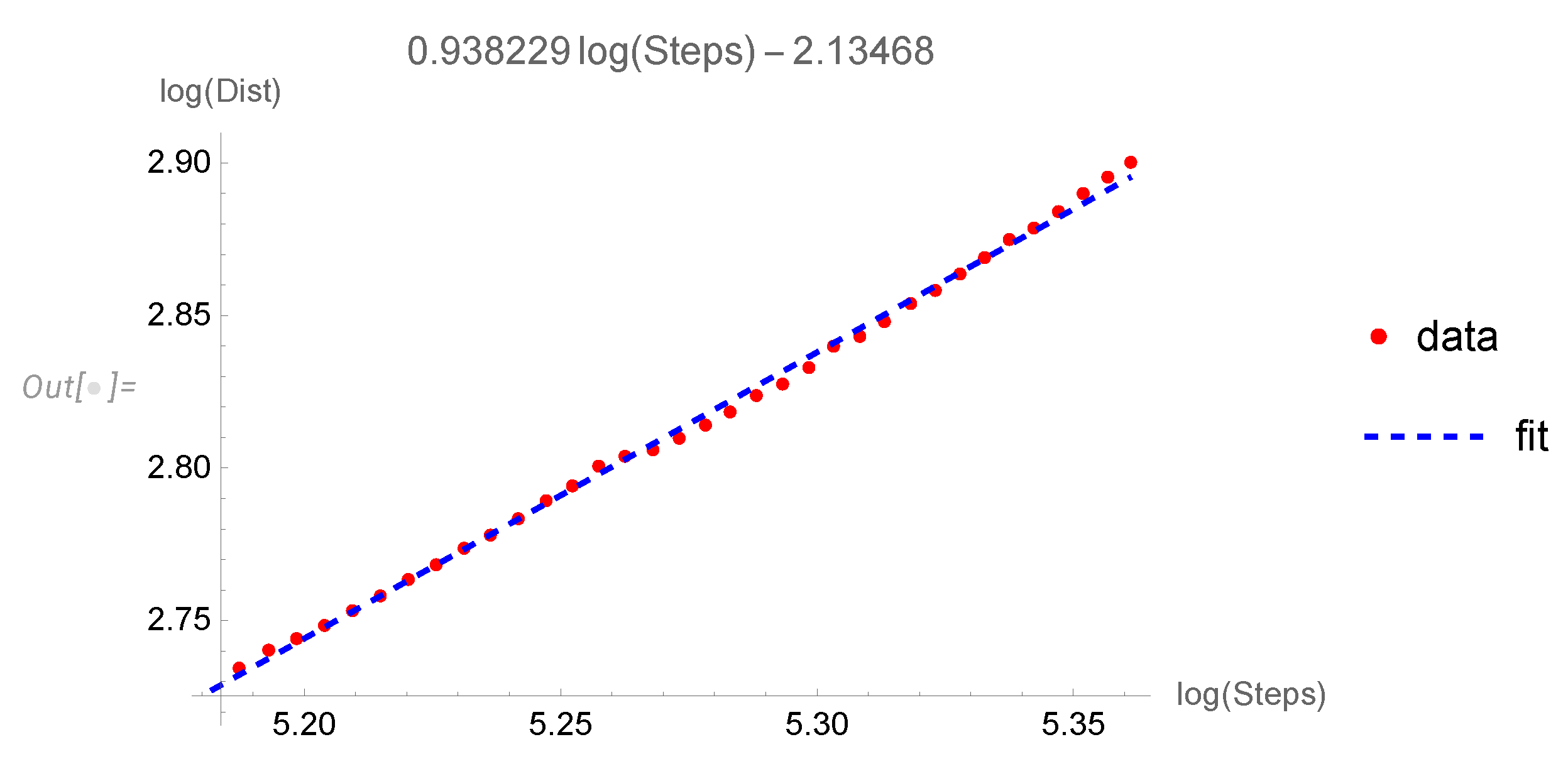
Figure 5.
The logarithmic plot of the CDF for the Euclidean length s of each step of our complex random walk. The tail of the CDF decays as , indicating the fractal distribution with power tail in PDF .
Figure 5.
The logarithmic plot of the CDF for the Euclidean length s of each step of our complex random walk. The tail of the CDF decays as , indicating the fractal distribution with power tail in PDF .
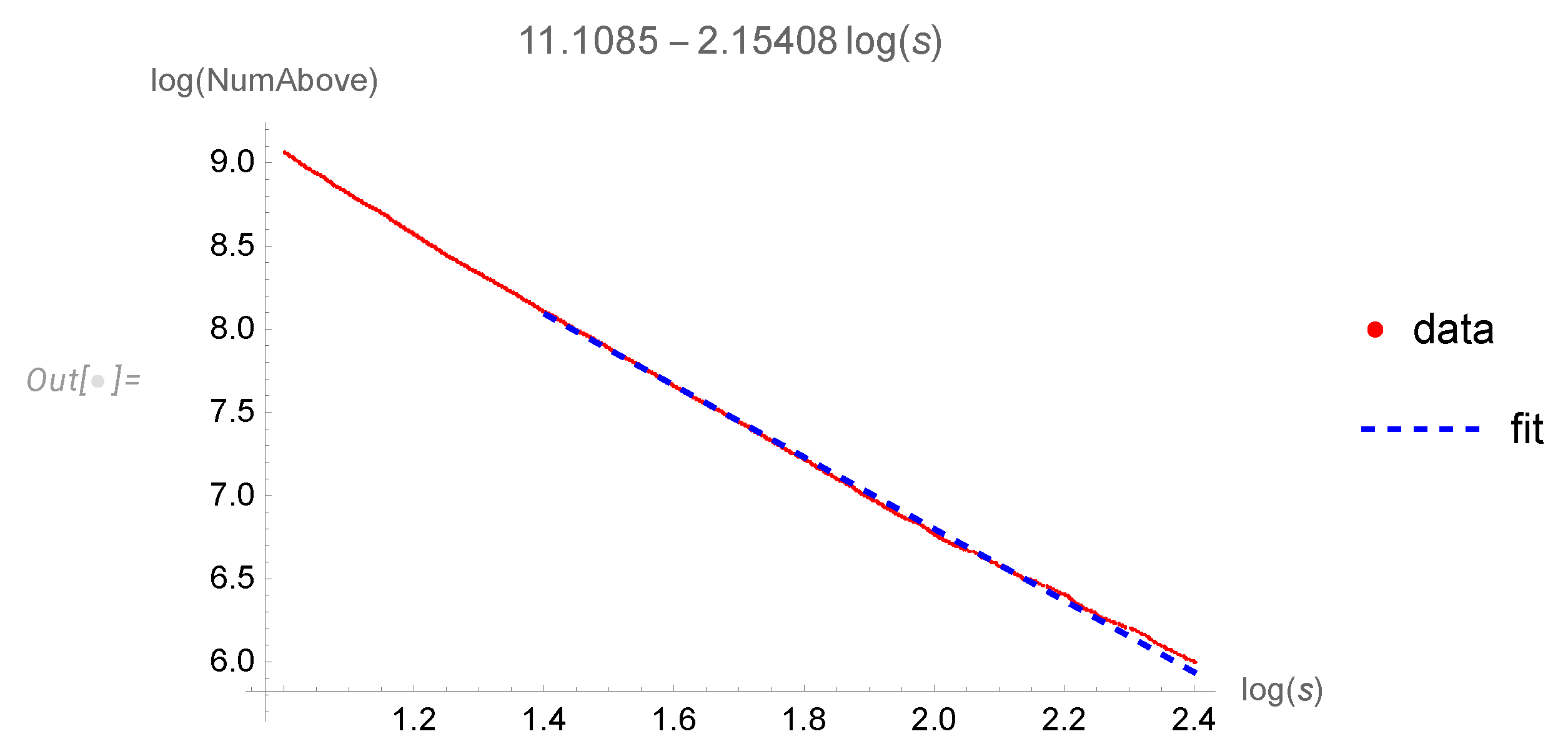
Figure 6.
The logarithmic plot of the CDF for the density. The tail of the CDF decays as , compatible with the power tail for PDF. The mean value of enstrophy and all higher moments diverge.
Figure 6.
The logarithmic plot of the CDF for the density. The tail of the CDF decays as , compatible with the power tail for PDF. The mean value of enstrophy and all higher moments diverge.
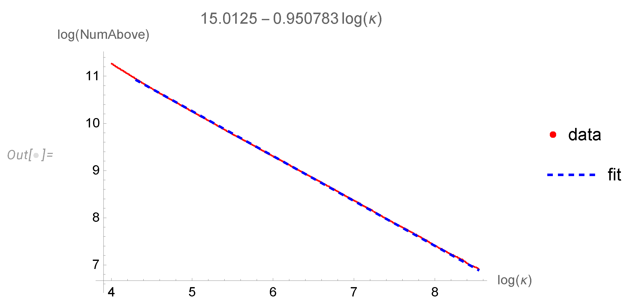
Figure 7.
Fitting noisy data for (red dots) by a power law . The best fit is a dashed blue line, corresponding to . This is how wrong laws can be "derived" by fitting noisy data.
Figure 7.
Fitting noisy data for (red dots) by a power law . The best fit is a dashed blue line, corresponding to . This is how wrong laws can be "derived" by fitting noisy data.
Disclaimer/Publisher’s Note: The statements, opinions and data contained in all publications are solely those of the individual author(s) and contributor(s) and not of MDPI and/or the editor(s). MDPI and/or the editor(s) disclaim responsibility for any injury to people or property resulting from any ideas, methods, instructions or products referred to in the content. |
© 2020 by the author. Licensee MDPI, Basel, Switzerland. This article is an open access article distributed under the terms and conditions of the Creative Commons Attribution (CC BY) license (https://creativecommons.org/licenses/by/4.0/).
Copyright: This open access article is published under a Creative Commons CC BY 4.0 license, which permit the free download, distribution, and reuse, provided that the author and preprint are cited in any reuse.


