Submitted:
10 May 2023
Posted:
12 May 2023
You are already at the latest version
Abstract
This primer provides an overview of the rapidly evolving field of generative artificial intelligence, specifically focusing on large language models like ChatGPT (OpenAI) and Bard (Google). Large language models have demonstrated unprecedented capabilities in responding to natural language prompts. The aim of this primer is to demystify the underlying theory and architecture of large language models, providing intuitive explanations for a broader audience. Learners seeking to gain insight into the technical underpinnings of large language models must sift through rapidly growing and fragmented literature on the topic. This primer brings all the main concepts into a single digestible document. Topics covered include text tokenization, vocabulary construction, token embedding, context embedding with attention mechanisms, artificial neural networks, and objective functions in model training. The primer also explores state-of-the-art methods in training large language models to generalize on specific applications and to align with human intentions. Finally, an introduction to the concept of prompt engineering highlights the importance of effective human-machine interaction through natural language in harnessing the full potential of artificial intelligence chatbots. This comprehensive yet accessible primer will benefit students and researchers seeking foundational knowledge and a deeper understanding of the inner workings of existing and emerging artificial intelligence models. The author hopes that the primer will encourage further responsible innovation and informed discussions about these increasingly powerful tools.
Keywords:
Generative Artificial Intelligence
; Large Language Models
; ChatGPT
; Bard
; Transformer Architecture
; Prompt Engineering
1. Introduction
Traditional artificial intelligence (AI) methods focused on detecting patterns, making decisions, modeling data, and classifying phenomena. Generative Artificial Intelligence (GAI) is an AI variant that can generate a variety of human consumable content such as natural language text, images, audio, code, and domain specific data. A large language model (LLM) is a special type of GAI that can generate natural language text in response to a natural language prompt. The convergence of massive amounts of data available on the Internet, ever-increasing computing capacity, and the discovery of an efficient language “transformer” architecture in 2017 led to breakthrough GAI capabilities in 2022 (Vaswani, et al., 2017). Specifically, ChatGPT, an AI chatbot from OpenAI, surprised much of humanity with its impressive capabilities of responding to natural language prompts. The invention illustrated that an artificial neural network (ANN), with as many connections as human brains has neurons, can generate human language uncannily well.
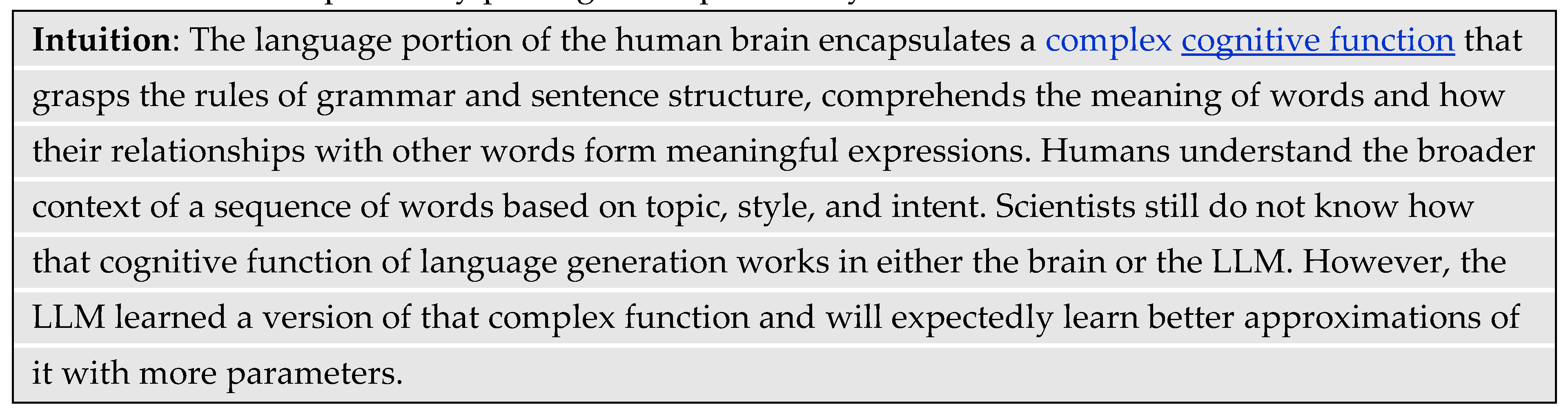
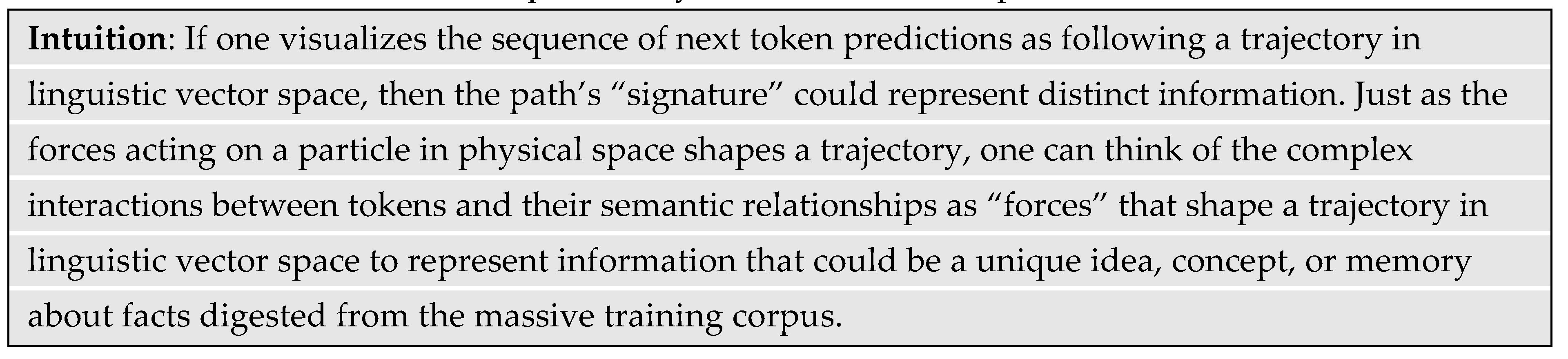
Scholars still do not comprehend how a finite and non-adaptive computing system can simultaneously capture the complexities of dozens of human languages plus the essence of all that it can chat about. This lack of understanding has led to misconceptions about how an LLM does what it is doing. A common misconception is that an LLM is simply a more capable autocomplete engine like those on smartphones and word processors that predict the next word. The developers at OpenAI posit that “somehow,” training the GAI model led it to discover underlying phenomena that represent cognitive processes in the human brain that enable coherent language generation and even some amount of reasoning (Wei, et al., 2023).
We do know that humans use language as a medium for expressing thoughts, ideas, and complex concepts. Hence, language proficiency enables humans to convey and receive information, formulate arguments, draw inferences from context, understand different perspectives, and solve various problems. Therefore, language helps humans acquire knowledge about the world, cultural norms, and social conventions. The human ability to reason helps in learning languages by understanding grammatical rules, inferring the meaning of unfamiliar words, and adapting that knowledge to different situations. GAI tools like ChatGPT give the impression that it can do all the above, and that has led to much controversy about what occurs inside its neural networks (Chomsky, Roberts, & Watumull, 2023). Research has also reported that LLMs have been developing certain “emergent” capabilities that their developers did not expect (Bubeck, et al., 2023).
The GPT acronym in ChatGPT stands for Generative Pretrained Transformer. The first word refers to a method of operation where the AI chatbot autoregressively generates or predicts one word at a time to best complete a coherent sentence. The second word refers to the method of developing the AI chatbot by pre-training a large language model (LLM) and then fine-tuning it to do domain specific tasks like answering questions. The third word refers to the usage of a transformer architecture discovered in 2017. ChatGPT became the world’s most viral software service with more than one million users registered within the first five days of its launch (Roose, 2022). OpenAI released GPT-4 on March 14, 2023. Microsoft Corporation partnered with OpenAI to incorporate GPT-4 into its Bing search engine (Peters, 2023). Google soon responded by launching a chatbot called Bard. Subsequently, there has been an explosion of research and commercial use cases for GAI models (Liu, et al., 2023).
The disruptive potential of LLMs to facilitate both good and malicious deeds have since generated extremes of excitement and apprehension (Bubeck, et al., 2023). History has taught us that humanity will continue to use innovative technology for both good (e.g., curing diseases), and bad (e.g., synthesizing untraceable computer viruses). This trend is likely to continue as developers march towards achieving artificial general intelligence (AGI), then artificial super intelligence (ASI), and beyond. A continued lack of understanding about how developers build LLMs to do what they do currently will further contribute to the fear and suspicion surrounding AI developments.
The goal of this primer is to help demystify how developers build LLMs like ChatGPT and Bard. The primer describes the various underlying theories and provides intuitive explanations about how they work. The author provides intuitive explanations of the technical descriptions in text boxes and highlights important or technical terminology in underlined font. The objective is to make this primer useful to a broad audience, and particularly to students and researchers who want to quickly become familiar with the underlying theories before undertaking further studies.
The organization of the remainder of this document is as follows: Section 3 explains the background natural language processing (NLP) methods that make up LLMs such as text tokenization, vocabulary construction, token embedding, context embedding with an attention mechanism, ANN function approximation, and the objective function in model training. Section 4 explains the architectural choices that enabled ChatGPT in the context of the background methods. Section 5 discusses the state-of-the-art methods of training and fine-tuning the models. Section 6 concludes this primer on how AI chatbots work. Section 7 offers a glimpse of future developments in GAI.
2. Background Methods
The public has long used products based on NLP techniques and language learning models. Examples include language translation apps, dictation transcription apps, smart speakers, and text to speech converters. Such technologies use ANNs as a key enabler. Familiar applications of ANN include face recognition in digital albums, biometric-based security systems, and music recognition. The architectures of modern LLMs contain common NLP elements that developers discovered over time. Figure 1 illustrates the basic building blocks and the flow of information through an LLM like the GPT series.
The training process repeatedly presents the model with massive amounts of word sequence examples so that it can incrementally learn how to predict the next word. The tokenize procedure converts the word sequence into symbols that represent a language more efficiently and aids in the creation of a fixed internal vocabulary for processing. Token embeddings and position encoding convert the fixed vocabulary to vectors of floating-point numbers that a computer can process. The attention mechanism produces contextualized vectors that encode the relevance of other tokens in the input sequence in establishing context for the sentence. The SoftMax function normalizes the contextualized vectors produced by the attention mechanism so that the ANN can discover and learn contextual patterns more efficiently. Normalization and residuals prepare the output vectors of the ANN for further processing without losing information during the sequential transformations. The objective function defines the statistical conditions and constraints for predicting the next token.
The architecture (Figure 1) operates slightly differently during training than it does during inference when predicting the next word. Training presents a word sequence randomly sampled from the training corpus and masks the next word while the model makes a prediction to maximize its objective function. The training algorithm then computes an error between the predicted and correct output to determine how it should incrementally adjust the model parameters to reduce the error gradually and continuously. The training algorithm then appends the correct word to the input sequence and continues the cycle of predictions and parameter adjustments. The process converges when the average error reaches a predetermined level. During inference, a trigger such as a query initiates the prediction of words, one at a time. The next subsections describe each of the building blocks in Figure 1 in greater detail.
2.1. Tokenization
Words have similar parts and other redundancies that algorithms can exploit to increase the efficiency of word representation. Tokenization algorithms do so by splitting a sentence into words, characters, and subwords called tokens. There are dozens of tokenization methods. Hence, this section focuses on the method used by ChatGPT. The goal of a tokenization algorithm is to retain frequently used words (e.g., “to,” “the,” “have,” “from”) and split longer or less frequently used words into subwords that can share prefixes and suffixes across words. OpenAI reported that on average, one token represented 0.7 words (Brown, et al., 2020).
There is an important distinction between using NLP techniques like tokenization to model topics in a corpus of text versus using them to build language models. The goal of the former is to distill the abstract topic from a collection of documents whereas the goal of the latter is to build a model that understands and generates natural language. Both endeavors use tokenization to help enhance the model’s ability to discover phrase patterns and word clusters. However, topic modeling uses two additional methods called stemming and lemmatization to create more structured and normalized representations of text to improve model performance. Stemming maps different forms of a word to a common base form to reduce the vocabulary size and handle variations of the same word. Lemmatization maps a word to a standard form based on its part of speech and meaning. Language models capture morphological information implicitly during the pretraining process without the need for additional preprocessing steps such as stemming or lemmatization.
2.2. Vocabulary
Simply building a vocabulary from all the unique tokens of the training corpus would be inefficient because languages consist of hundreds of thousands of unique tokens. The Oxford English dictionary alone has more than 600,000 words (Stevenson, 2010). Creating an efficient language model requires a much smaller and fixed-size vocabulary. Dozens of methods are available to build a vocabulary. GPT-3 uses a method called byte-pair encoding (BPE) to build a fixed size, static vocabulary of approximately 50,000 tokens. The method compresses text based on the statistics that significantly fewer unique characters make up tokens than words make up sentences. BPE executes the following procedures: pre-processing, token frequency distribution (TFD), vocabulary initialization, merge iteration, vocabulary finalization, and post-tokenization.
Pre-processing: lowercase the corpus for search consistency; remove extra spaces; remove non-alphanumeric characters and normalize text by removing diacritical marks and using consistent spelling across language variants.
Token frequency distribution: convert the corpus to tokens and extract a table of unique tokens along with their frequency of occurrence. Hence, the table represents the TFD needed to build the vocabulary.
Vocabulary initialization: build a base vocabulary using 256 bytes from the 8-bit Unicode Transformation Format (UTF-8). The first 128 symbols of UTF-8 correspond to the standard English ASCII characters. UTF-8 is the dominant encoding on the internet, accounting for approximately 98% of all web pages (W3Techs, 2023). Using UTF-8 bytes assures that the symbols in the base vocabulary map all unique characters in the TFD.
Merge iteration: calculate the occurrence frequency of all pairwise combinations of symbols in the base vocabulary by counting their paired occurrence across all tokens of the TFD. Hence, multiple tokens will contain the same symbol pair. Iteratively assign an unused symbol to the highest frequency symbol pair and append it to the base vocabulary. As the merging continues, the algorithm begins to assign unique symbols to increasingly longer concatenations of tokens to form n-grams where n is the number of characters of merged tokens (Sennrich, Haddow, & Birch, 2015). The iteration stops after the vocabulary reaches a predetermined size.
Vocabulary finalization: the final vocabulary will have symbols representing individual bytes, common byte sequences, and multi-byte tokens. The procedure finalizes the vocabulary by adding non-linguistic tokens such as [PAD] and [UNK] to accommodate padding and unknown tokens, respectively, as well as other special tokens to deal with other situations.
Post-tokenization: convert the pre-tokenized input corpus by replacing tokens with their matching n-grams in the final vocabulary.
The BPE method has the capacity to encode a diverse range of languages and Unicode characters by efficiently capturing sub-word structure and distinct meaning across similar words. The method can also effectively tokenize out-of-vocabulary words so that the model can infer their meaning. The BPE text compression method is also reversible and lossless. The reversible property assures that the method can translate the symbolized token sequence back to the natural language of words. Lossless in the sense of compression methods means that there is no loss of information during the compression that will lead to ambiguity during the decompression.
2.3. Token Embedding
A token embedding method converts the token symbols to number vectors that a computer can use to represent tokens in a computational number space. A desirable feature of token embedding is to reflect the position of the token in the vocabulary for lookup. That way, when the decoder outputs a probability vector for the predicted token, the maximum value will correspond to the position of the predicted token. Therefore, the ideal vector would be a one-hot-encoded (OHE) where all positions contain a “0” except for the position of the encoded token where it contains a “1.” Hence, the size of the OHE vector is equal to the size of the vocabulary. However, an OHE vector is too sparse to carry sufficient syntactic or semantic information about a token and how it relates to other tokens in a sequence. Hence, GPT-3 constructed a denser number vector for information processing and then converted that to an OHE vector to lookup the predicted token.
GPT-3 learned the vector embeddings for each token during training. The dimension of the number vector is 12,288, which is a hyperparameter that is approximately one-quarter the size of the vocabulary. Hyperparameters are settings that the model architects pick because they are not learnable during the training process. Each dimension of the embedding vector is a continuous floating-point number. An embedding matrix converted the OHE vector of the vocabulary to embedded token vectors. Hence, the number of rows in the embedding matrix is equal to the vocabulary size. The number of columns in the embedding matrix is equal to the dimension of the embedded token vector. GPT-3 trained a linear neural network to learn the matrix that converts the token symbols to number vectors.
2.4. Positional Encoding
Prior to the transformer architecture, the state-of-the-art NLP methods were recurrent neural networks (RNNs) and long short-term memories (LSTMs). RNNs process sequential data by maintaining a hidden state that updates with each new input in the sequence. The state serves as a memory that captures information from previous inputs. However, this dynamic memory element tends to lose information about long-range dependencies in the sequence. That is, after a few hundred words, the internal state begins to lose context about the relevance of earlier tokens. LSTMs are a type of RNN designed to overcome some of the long-term memory issues of RNNs. The LSTM architecture incorporates input, output, and “forget” gates in a more complex cell structure to control the flow of information. Those complex structures are not important to understand here except that RNN and LSTM architectures natively process sequential data, so word ordering is inherently encoded.
Architectures that inherently process information sequentially are difficult to parallelize so that they can exploit parallel computing methods to achieve higher efficiency and speeds. Conversely, the transformer architecture did not use the feedback type connections of RNNs and LSTMs so their processing elements could be parallelized. However, in so doing, the transformer architecture lost the sense of word ordering. The ordering and dependencies of words are important for language understanding. This problem introduced the need for positional encoding. Positional information helps the LLM to learn relationships among tokens based on both their absolute and relative positions in a sequence. There are dozens of methods to encode token positions. GPT-3 learned how to add position encoding to tokens by adapting the parameters of its ANN during training to identify an undefined approach that is consistent with the objective function (Brown, et al., 2020).

2.5. Attention Mechanism
Token and position embeddings capture syntactic information such as grammatical form and structure. However, those embeddings do not necessarily capture semantic information such as contextual meaning and tone based on other tokens in a sequence. Figure 3 provides an example of how a single word difference can change the contextual meaning of a sentence. The sentences “The dog sat on my couch because it was soft” and “The dog sat on my couch because it was tired” share the same words and ordering, except the last word. The last word completely changed the meaning of the two sentences. Humans intuitively know that the word “it” in the first sentence refers to “couch” because of the context “soft” whereas “tired” in the second sentence refers to “dog” because of human intuition that a couch cannot feel tired.
The self-attention mechanism learns to capture contextual meaning based on how certain tokens in a sequence “attend” to other tokens. The mechanism does so by creating contextualized versions of each token by adding portions of the embeddings of other tokens that it needs to express. The amount of expression added to a token at a given position is based on a normalized weighted distribution of all the tokens in the sequence.
Figure 4 provides an example in two-dimensional vector space to illustrate the effect that the self-attention mechanism has when contextualizing word embeddings. In this example, the contextualized token “Machine.a” expresses 70% of the token “Machine” and 30% of the token “Learning” whereas the contextualized token “Learning.a” expresses 70% of the token “Learning” and 30% of the token “Machine”. Hence, the normalized weight distribution for the first token is (0.7, 0.3) and that for the second token is (0.3, 0.7). The effect is that the two contextualized token vectors move closer to each other in the embedded vector space.
Bahdanau et al. (2014) first introduced the attention mechanism in 2014 to dynamically focus on various parts of an input sentence during a translation task (Bahdanau, Cho, & Bengio, 2014). However, it was not until the introduction of the transformer architecture in 2017 that the attention mechanism gained significant recognition (Vaswani, et al., 2017). The first transformer architecture modeled the dependencies between tokens in a sequence without the need to rely on previous state-of-the-art methods like recurrent neural networks and convolution neural networks. Moreover, the transformer parallelized operations to be more computationally efficient and faster by using many graphical processing units (GPUs) at once. The transformer architecture has since become the foundation for state-of-the-art LLMs like ChatGPT and Bard.
Figure 5 illustrates the flow of vector transformations from the input token embeddings to the contextualized vectors. The model packed the input sequence of token embeddings into a matrix X. The attention mechanism then computed co-relevance scores for every unique pair of tokens as the dot product of their representation vectors. The representation vectors are three projection vectors of the input token embeddings called the query, key, and value vectors. During training, the model learned the parameters of a linear network (WQ, WK, WV) to produce the three projection matrices Q, K, and V that pack the corresponding projection vectors. Each box in Figure 5 represents an operation or a matrix of the dimensions shown. The variable n is the number of tokens in the input sequence, and dq, dk, dv are the dimensions of the query, key, and value vectors, respectively. The attention mechanism typically downsizes the dimension of the three projection matrices from the original dimension of the input matrix X. A later section will discuss the intuition behind the dimension change.
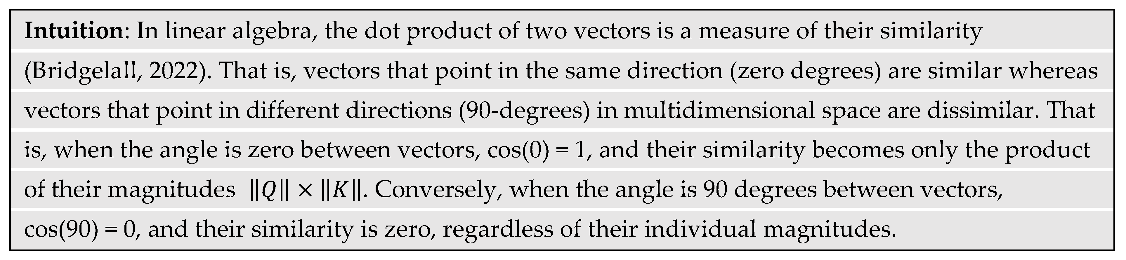
The dot product, also called the inner product, between two equal length n-dimensional vectors Q = [q1, q2, ..., qn] and K = [k1, k2, ..., kn] is a scalar value s where
and || . || is the magnitude operator (Bridgelall, 2022).
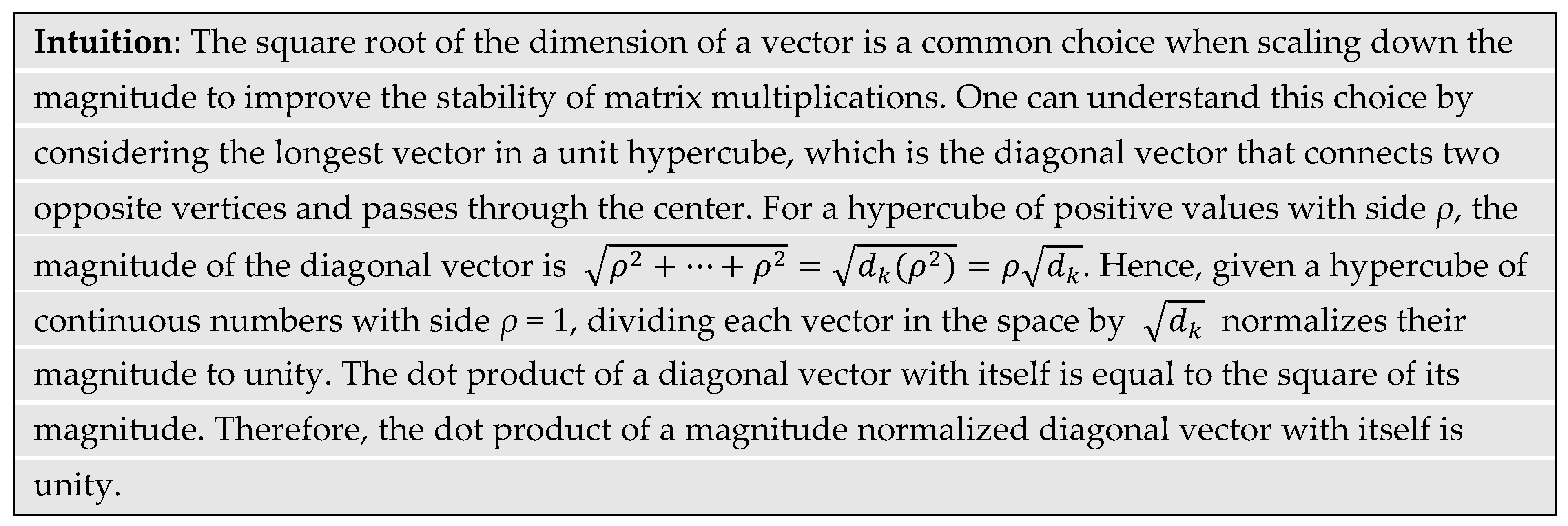
Formally, the attention mechanism computes
where the scaling factor λ = in the GPT-3 model (Brown, et al., 2020). That is, co-relevance scores form the weights in a weighted sum of value vectors V that produce the contextualized vectors in a matrix Z. The matrix multiplication Q × KT directly computes the dot product or co-relevance scores, which is a square matrix of dimension n × n. The co-relevance scores are for every pairwise combination of query and key token representation vectors in the input sequence. The downstream SoftMax function, discussed in the next subsection, normalizes the scores to produce a normalized distribution of weights used to produce the weighted sum of value vectors.
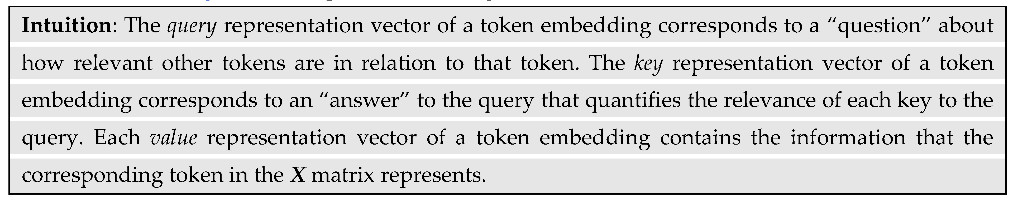
Figure 6 explains how the matrix multiplication is equivalent to generating an n × n square matrix S of co-relevance scores or dot products. As highlighted in the figure, the first entry in row 1, column 1 is the dot product between row 1 from the Q matrix and column 1 from the transposed K matrix. To generalize, the scalar value in row i, column j of the S matrix is the dot product between row i of the Q matrix and column j of the K matrix.
In general, the dot product of token vectors with themselves will tend to have the highest co-relevance scores, which are located along the diagonal of the S matrix. Non-identical token pairs with high co-relevance will have high scores that are located off the main diagonal. Figure 7 illustrates a matrix of co-relevance scores for every pairwise combination of input tokens in the matrix X. The light color along the diagonal indicates high co-relevance scores whereas the darker colors indicate lower co-relevance scores.
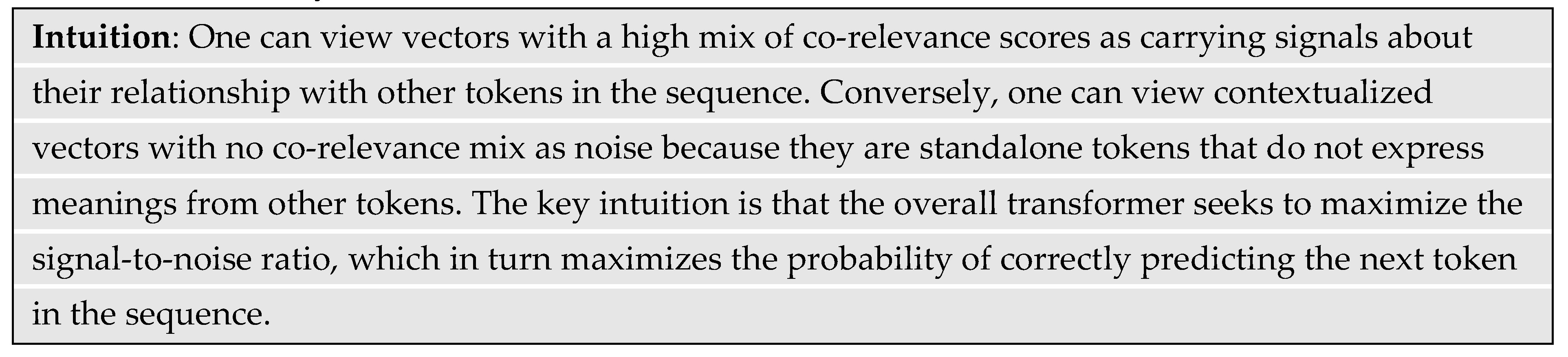
Some contextualized vectors in the output matrix Z will have strong mixes of co-relevance scores whereas others may have no co-relevance mix.
2.6. SoftMax Function
The SoftMax function normalizes the co-relevance scores so that they are all positive and sum to unity. The formula is
where z is a d-dimensional vector of values z = (z1, ... , zd) and σ(z)i is the weight associated with element i in the vector. A problem with the SoftMax function is that it biases the largest weights towards the largest elements of the vector, which leaves little room to distribute the remaining weights across the smaller elements. For example, Figure 8 plots the SoftMax values for a 5-dimensional vector (d = 5) for the values at positions one (X1) and five (X5). The example vector is X = [1, 1, 1, 1, 2].
The SoftMax output or weight distribution is [0.15, 0.15, 0.15, 0.15, 0.40] with no scaling, which is with λ = 1. Hence, without scaling down the vector, the weight for element X5 is 2.7 times the weight of the other elements whereas the element value is only 2.0 times that of the others. As the scaling factor increases beyond 1.0, the distribution of the weights begins to equalize towards a uniform distribution with weights equal to 1/d or 1/5 = 0.2 for each element. Therefore, the best scaling factor will balance the tradeoff between weight dominance and weight uniformity. In this example, the scaling factor of appears near the knee of the two curves and provides a more representative distribution of weights as [0.18, 0.18, 0.18, 0.18, 0.28]. That is, the weight of element X5 is now 1.6 times instead of 2.7 times the weight of the other elements.
2.7. Artificial Neural Networks
An ANN is a computing model invented in the early 1950’s to approximate a basic function that scientists believed the biological neuron of a human brain implements (Walczak, 2019). However, a lack of computing capacity at the time of ANN development limited its scaling for general computational tasks. More recently, the invention of the graphical processing unit (GPU) that can efficiently do matrix operations helped to accelerate the utility of ANNs in NLP applications (Otter, Medina, & Kalita, 2020). Gaming platforms initially drove the adoption and proliferation of GPUs, and subsequently cryptocurrency mining and blockchain development further accelerated demand. The ANN is the most crucial element of an LLM because it helps the overall architecture learn how to achieve its objectives through training. Therefore, the subsections that follow describe simple ANNs in detail to provide an intuitive understanding of how they work and how they can scale to learn more complex functions.
2.7.1. Basic Architecture
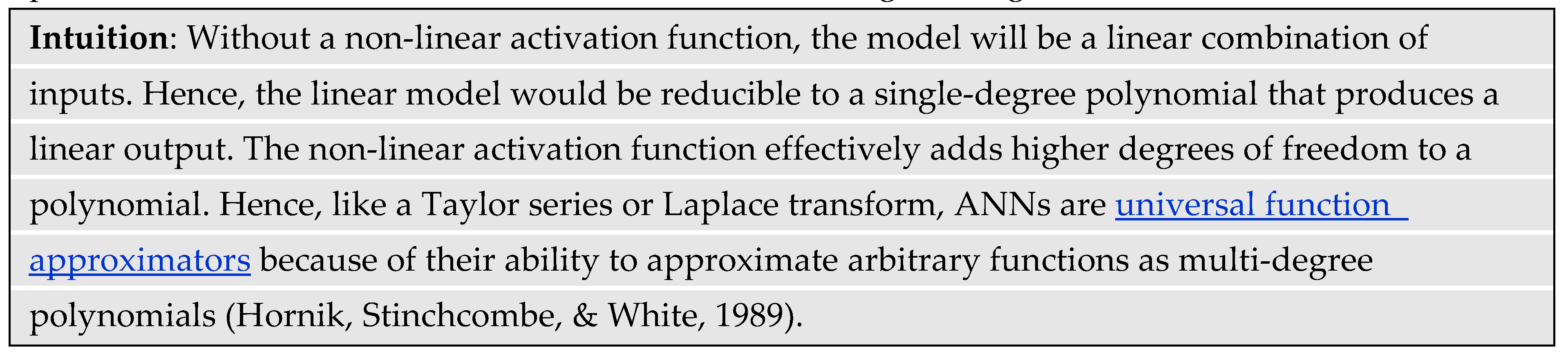
The basic architecture of an ANN is an input layer of artificial neurons or nodes, one or more hidden layers of nodes, and an output layer of nodes. The node loosely mimics a biological neuron by calculating a weighted sum of its input signals plus a bias signal. The result of the weighted sum passes through a non-linear “activation” function to produce the node’s output. Without a non-linear activation function, the ANN reduces to linear operations. The literature refers to the type of ANN used to build LLMs as a feed-forward neural network (FFNN). That distinguishes it from other architectures like recurrent neural networks (RNNs) that incorporate feedback signals from intermediate output layers to earlier layers.
Figure 9 shows a small FFNN with one input node taking the value x, and one output node producing the value y. There are two inner or hidden layers consisting of two nodes each (2H × 2H) with labels Hij. The labels for the weights and biases are wij and bij, respectively. In this example, the i and j values represent rows and columns of the ANN structure, respectively.
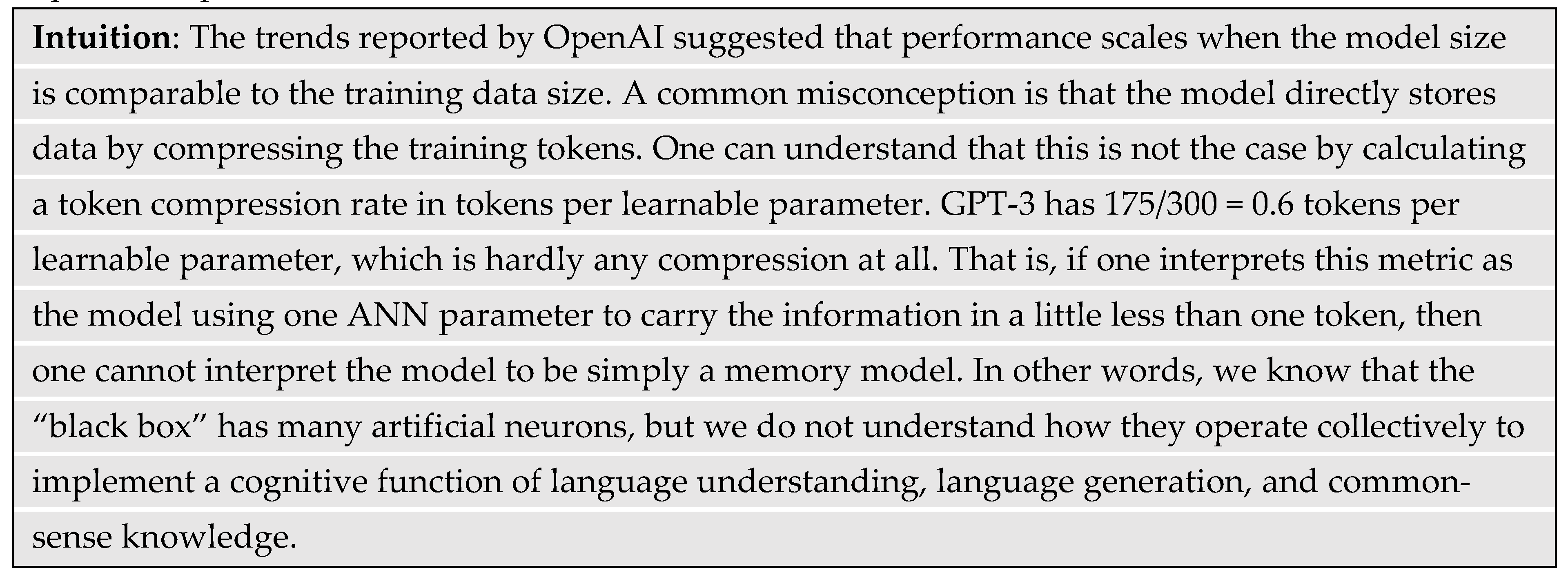
In general, a larger ANN has multiple inputs and multiple outputs, with each corresponding to a different feature in the input and output data. The nodes operate collectively to produce an arbitrary function of the input. The literature refers to the collection of weights and biases as parameters of the network. The developers of GPT-3 scaled the basic architecture of Figure 1 to 175 billion parameters (Brown, et al., 2020). For perspective, the human brain has approximately one hundred billion neurons, each with thousands of synapses connecting it to other neurons or cells (Wolfram, 2002). This suggests that, at the time of this writing, LLMs are far from having the equivalent number of learnable parameters as the human brain, which can learn in real-time using less energy.
2.7.2. Activation function
The activation function preserves or diminishes the weighted sum of input signals to a node. This non-linear action collectively activates neural pathways to propagate a signal along unique paths through the network. From a mathematical perspective, the activation function introduces non-linearity which enables the network to collectively learn a complex function. Early ANNs used the sigmoid function for activation. However, later research found that the sigmoid function led to slow training convergence. That is, during network training, an algorithm called backpropagation calculates incremental adjustments to the parameters so that the output gradually gets closer to the true value. The backpropagation algorithm tracks the output error, which is the difference between the current predicted token vector and the correct token vector. If further incremental adjustments to the parameters do not result in further error reduction, then the training could be stuck at a local minimum rather than a global minimum. Subsequent research found that using a simpler rectified linear unit (ReLU) activation function resulted in faster network training and better generalization performance (Krizhevsky, Sutskever, & Hinton, 2017). Generalization refers to the predictive performance of trained models on data never seen during training.
The sigmoid function is
and the ReLU function is
The ReLU function implements a deterministic node dropout (zeroing of the output) for negative values and an identity function (replicating the input) for positive values. Subsequent research found that a Gaussian Error Linear Unit (GELU) can replace deterministic dropout with stochastic dropout and then transition to the identity function to yield better convergence (Hendrycks & Gimpel, 2016). The GELU function is
where P is a probability, and the features of the vector X are N(0, 1) distributed. The notation N(μ, σ) refers to a normal distribution with mean μ and variance σ. A disadvantage of the GELU function is its computational complexity relative to the ReLU function. However, Hendrycks and Gimpel (2016) suggested the following function as a fast approximation (Hendrycks & Gimpel, 2016):
Figure 10 plots the three activation functions for comparison. The ReLU has no signal “leakage” to the output for negative input values. Conversely, the Sigmoid and GELU have positive and negative output leakage, respectively, for negative input values. Although the ReLU is much simpler among the three activation functions, it has a discontinuity at zero when taking the derivative as part of the backpropagation algorithm. Therefore, the training algorithm must define the derivative at zero as either 0 or 1.
2.7.3. Multi-Layer ANN
Scaling an ANN to learn more complex functions like a natural language involves increasing both the width and depth of the nodal structure and the degree of connectivity among the nodes. One can visualize the width as a vertical arrangement of nodes and the depth as horizontal layers of the vertical arrangement. An ANN creates an arbitrary function by learning parameters that produce intermediate outputs at each node that then combine to piece-wise approximate a complex function. Figure 11 shows how the ReLU function changes by adjusting various weights and bias parameters.
The sub-functions at the output of the first layer of nodes with ReLU activation cannot leave the x-axis. However, adding another inner layer of nodes with ReLU activation adds flexibility to create more complex sub-functions that can leave the x-axis.
The following example of approximating a sine wave offers some insight into how sub-functions of the ReLU activation combine to create the output. Figure 12 shows a small ANN within one hidden layer consisting of three nodes with ReLU activations. The vector representations for the input weights w(i), biases b(i), and output weights w(u), are
The vector of values produced from the hidden layer H(1) is
where the dot is the dot product operator and ψ is the ReLU activation function.
The output y is
Putting it all together, the ANN in this scenario implements a function that produces a single scalar output y that depends on the weights, biases, and the non-linear activation function where
Figure 13a shows how the learned parameters approximated a sine wave y = sin(π·x) within the x range of [-1, 1].
The learned parameters were
Figure 13b shows the intermediate inputs to the output node y from the three paths through the network.

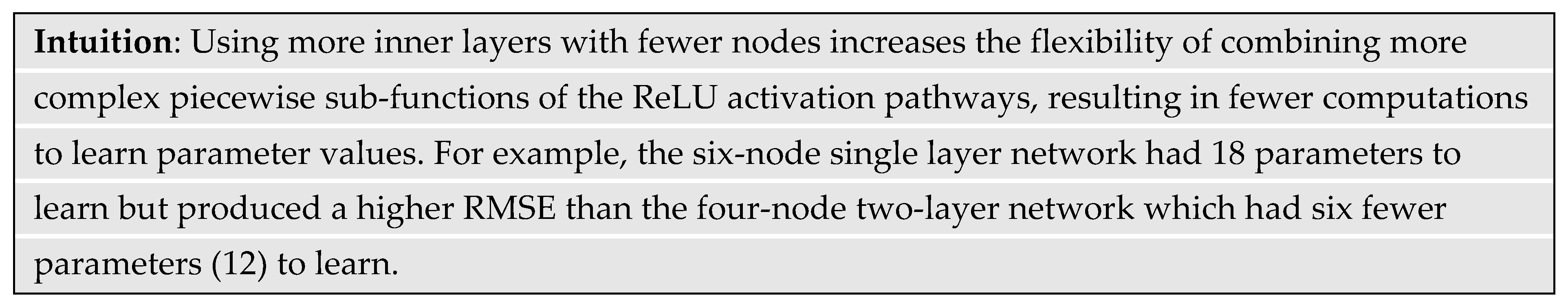
The root-mean-square-error (RMSE) for the 1H: 3×1 network with three learned parameters was 0.37. Increasing the number of inner nodes to six increased the number of learnable parameters to 18 but the RMSE declined to 0.141, which is a factor of 2.6. Figure 14a shows the function approximation and Figure 14b shows the trend in RMSE decrease with each additional inner node. The observed trend was that moving from two to three inner nodes produced the greatest decline in RMSE, but the subsequent decline in errors was only asymptotic.
So, changing the ANN architecture by adding one additional inner layer as shown earlier in Figure 9 resulted in a lower RMSE of 0.153. That RMSE was between the value achieved by the five- and six-node single layer networks. The two-layer network with two nodes per layer computed the following function of 12 parameters:
The trained weights were:
2.7.4. Network Training
During training, the network incrementally learns the value of each parameter that best predicts the output from a given input. Also, during training the backpropagation algorithm incrementally adjusts all the model parameters in a direction that gradually decreases the error with each training iteration. A differentiable loss function of the error enables the backpropagation algorithm to compute gradients. That is, a derivative of the loss function with respect to a parameter produces a gradient that tells the algorithm the direction to adjust that parameter to reduce the error. The derivative uses the chain rule of calculus to propagate parameter adjustments backwards from the output. The adjustments are incremental to make it easier for the algorithm to find a global minimum instead of a local minimum of the loss function. Backpropagation uses a method called stochastic gradient descent (SGD) that adds randomness to the process which further prevents the error from being stuck in a local minimum.
The amount of adjustment is a hyperparameter called the learning rate. A training epoch is one complete pass through the training data. Training involves multiple epochs to achieve convergence. The term convergence in the context of machine learning is the point at which the prediction error or loss is within some predetermined value range where further training no longer improves the model. The point of convergence is equally applicable to self-supervised and supervised types of machine learning. Perplexity is another measure often used to determine when the machine has learned sufficiently well to generalize on unseen data. The goal is to minimize perplexity, which indicates that the model consistently assigns higher probabilities to the correct predictions.
2.8. Residual Connections
Microsoft research found that training and testing errors in deep models tend to plateau with each additional layer of the ANN (He, Zhang, Ren, & Sun, 2016). The vanishing gradient problem became more pronounced with increasingly deep models. That is, the gradients calculated to adjust parameters can become excessively small. For example, when the backpropagation algorithm uses the derivative chain rule to multiply a series of values that are less than 1.0, the result can be exceedingly small. For instance, a value of 0.1 multiplied only 5 times (once per layer) yields (0.1)5 = 0.00001. The training slows or even halts when gradients become excessively small because parameter updates during backpropagation, which is based on the size of gradients, become correspondingly smaller in layers closer to the input.
Microsoft research found that making a neural network layer fit a residual mapping of the input to the output instead of fitting a new learned function helped to address the degradation problem (He, Zhang, Ren, & Sun, 2016). Formally, if H(x) is an underlying mapping that enables a layer to contribute to generalized learning, then the residual (difference) will be F(x) = H(x) – x. Algebraically, the underlying mapping becomes H(x) = F(x) + x. The interpretation here is that a residual is simply adding the layer input x back to its output, which is a learned residual function F(x) that contributes to the underlying mapping. Hence, when the output is close to the input, the residual (difference) will be small. The study hypothesized that if the optimum mapping for one or more layers turned out to be the identity (pass through) function, then the network would be more adept at pushing the residuals towards zero than it would be at fitting a new identity function at each layer to propagate the input signal (He, Zhang, Ren, & Sun, 2016). Practically, the residual connection forms a shortcut around one or more layers of the vector mappings.
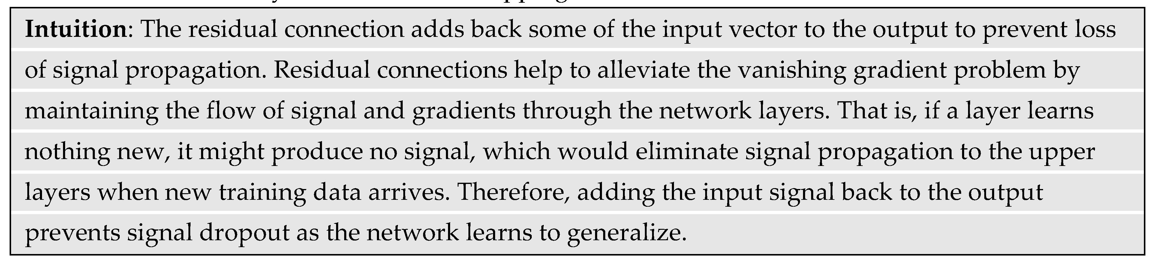
Figure 15 extends the example from Figure 4 to show the residual vector formed from the summation of the original vector “Machine” and its attention version “Machine.a” as “Machine.r”. Similarly, the figure shows the residual vector formed from the summation of the original vector “Learning” and its attention version “Learning.a” as “Learning.r”. The effect of forming the residual was to boost the attention vector magnitudes towards the original vectors. That is, if learning nothing new resulted in zero signal propagation, the residual connection shifted the input representation slightly without significantly modifying the token representation so that learning can continue without degradation.
2.9. Layer Normalization
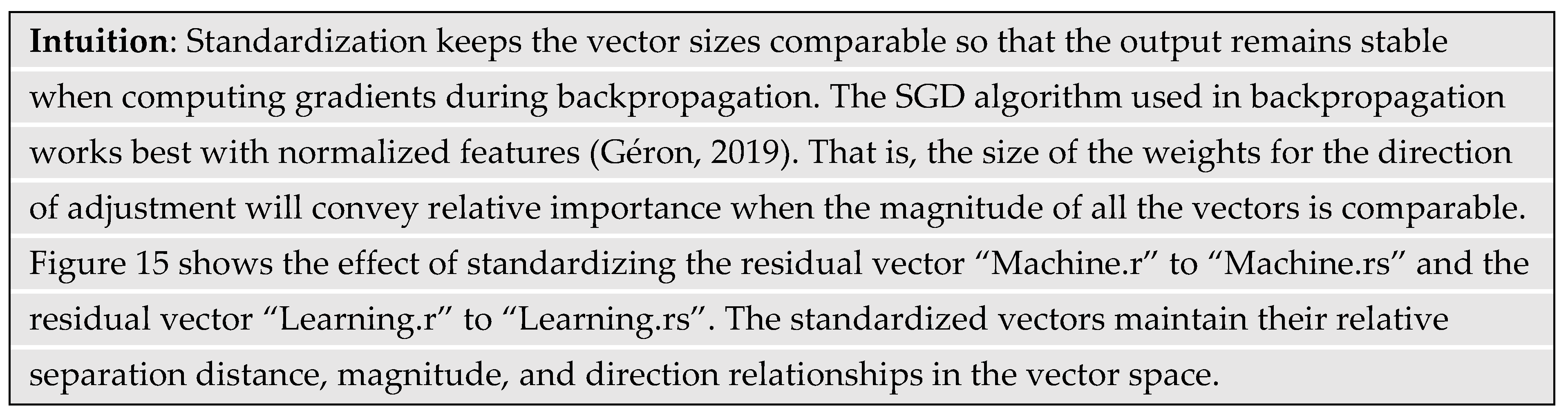
When training deep networks, in addition to the vanishing gradient problem, the gradients calculated to adjust parameters can also explode if they get too large. For example, multiplying the number 10 only five times yields 105 = 100,000. Large gradients make the training unstable because of parameter oscillations that prevent training convergence. Normalization helps to prevent both vanishing and exploding gradients while increasing training speed and reducing bias (Ba, Kiros, & Hinton, 2016). GPT-3 uses a method called layer normalization, which standardizes the vectors of all inputs from a single training batch before presenting them to the nodes of a layer, and prior to the activation function.
The standardization process first computes the mean and standard deviation across all the elements of all vectors in a training batch. The procedure then subtracts the mean from each element of all vectors (also called shifting), and then divides by the standard deviation (also called scaling). The result is a collection of elements from all the layer vectors that have a distribution with zero mean and unit variance.
2.10. Objective Function
The goal of classical statistical language modeling was to learn the joint probability of word sequences. However, that was an intrinsically difficult problem because of the large dimension of possibilities. Bengio et al. (2000) addressed this issue by pioneering a technique to train language models by predicting the next word in a sequence (Bengio, Ducharme, & Vincent, 2000). Mathematically, training tunes the model parameters Θ to maximize a conditional probability P in a loss function L1 where
and C = {c1, ..., cn} is a set of n tokens in a training batch that make up characters, words, and subwords in the sequence (Radford, Narasimhan, Salimans, & Sutskever, 2018). The input context window of the model holds a maximum of k training tokens at a time. The training technique is self-supervised because it masks the next token in a training sequence prior to its prediction. The SGD algorithm backpropagates incremental adjustments to the model parameters so that the error between the predicted and correct token gradually declines to some predetermined level (Géron, 2019). Instead of training on a single example at a time, the model trains simultaneously on a batch of examples. The loss function is the average of the differences between the predictions and the correct tokens.
3. LLM Methods
This section describes the overall architecture of GPT-3 and demonstrates how it uses the various NLP techniques discussed in the previous section. Figure 16 provides an overview of the GPT-3 architecture. The left side of the diagram shows the token flow from their vector embeddings at the bottom to their transformation into contextualized vectors and output probabilities at the top. The model first transforms an input sequence of tokens in the context window to embedded vectors. The model then adds positional encoding so that the decoder has information about their order and separation distance in the input sequence. The model then packs the transformed input tokens into a matrix X that the decoder uses during training and inference.
During training, the model learns the parameters of its ANN in the decoder stack to maximize the probability of correctly predicting the next token in the input sequence. After training, the model has learned the underlying phenomenon that produced all the text corpus used to train it. That is, the model learned general knowledge from the training examples to generate responses that are consistent with human understanding, within the context of the prompt.
During inference, the model gives the impression that it understands the syntax, semantics, and context of a prompt sufficiently well to produce a sensible and informative response. The inference is statistical in nature because once the model decides on a response, it begins to generate natural language that conveys the essence of the response, constrained by choosing the next word that is consistent with a pre-determined probability setting. That is, downstream developers can set a hyperparameter called “temperature” that tells the model what probability level to use when predicting the next word in its response. A temperature of zero tells the model to pick the next word that is associated with the highest probability whereas a higher setting causes the model to produce more “creative” responses by picking lower probability next words.
Predicting the next word based on probabilities led to limitations of LLMs. For example, if the prompting is ambiguous or lacks context, the model can confidently produce inaccurate or nonsensical responses called hallucinations that still seem plausible. The subsections that follow discuss each part of the architecture in greater detail by referring to the explanations of the background methods discussed in the previous section.
3.1. GPT Architecture Overview
Language understanding requires knowledge about word syntax, word position in a sequence, semantics, and overall context. An LLM transforms every word in a sentence to encode those key language concepts. The token embedding and position encoding schemes capture mostly the syntactic and grammatical structure among words. As discussed previously, the attention mechanism captures the semantic and contextual meaning of the input sequence. The middle of Figure 16 shows an exploded view of the first decoder in the stack of decoders. The right side of Figure 16 shows an exploded view of the attention mechanism described earlier (Figure 5). The first decoder layer performs the transformation:
where the matrix X = (x-n, ..., x-1) contains the token symbols x in the context window of size n. GPT-3 uses n = 2048 (Brown, et al., 2020). The matrix We is the token embedding matrix, and Wp is the position encoding matrix. Figure 16 annotates the dimension of each matrix in the superscript indicated next to the output of a functional block. The dimension of each token vector is d. GPT-3 uses d = 12,288 (Brown, et al., 2020).
The decoders in subsequent layers of the stack of N decoders process the output of the previous decoder. The last layer in the decoder stack produces the contextualized token matrix Z. The linear network at the output of the decoder stack converts the contextualized token vectors to logit vectors in matrix Y where the dimension of each vector is the length of the vocabulary indicated as m. GPT-3 uses m = 50,257 (Brown, et al., 2020). The SoftMax function normalizes each logit value to a probability distribution over the vocabulary. Therefore, the position of the peak value points to the position of the predicted next token in the vocabulary if the temperature setting is zero. During inference, the decoder predicts tokens in time steps, one token at a time. The decoder adds each predicted token to the input context window to build the input sequence and then predicts the next token based on the updated objective function. The looping terminates when the input receives a special stop token.
The exploded view of the decoder in the middle of Figure 16 shows that the output of the attention mechanism feeds into a residual connection, which then feeds into a layer normalization block that standardizes the batch of co-relevance vectors. The FFNN (FFn) at each token position independently adjusts the co-relevance vector at that position to further refine its meaning in preparation for more self-attention processing in later decoder layers.
3.2. Multi-headed Attention
The GPT architecture uses more than one block of attention mechanism per decoder layer. GPT-3 uses h = 96 attention heads (Brown, et al., 2020).
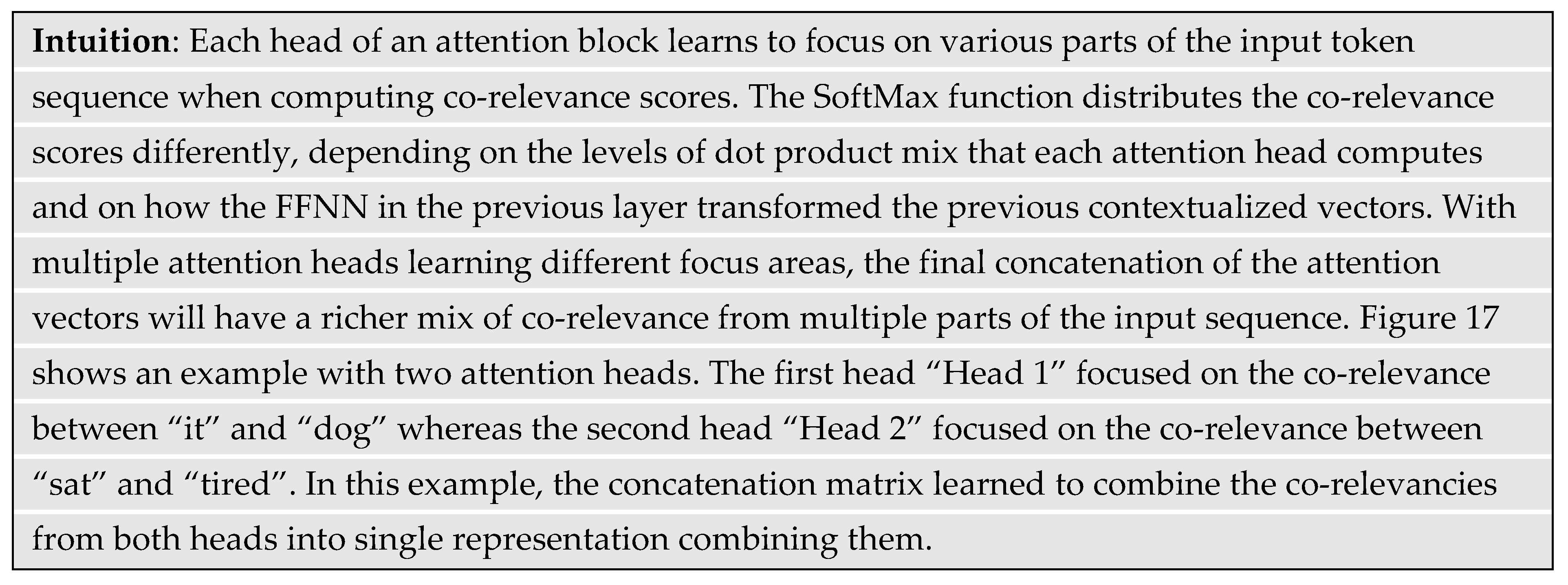
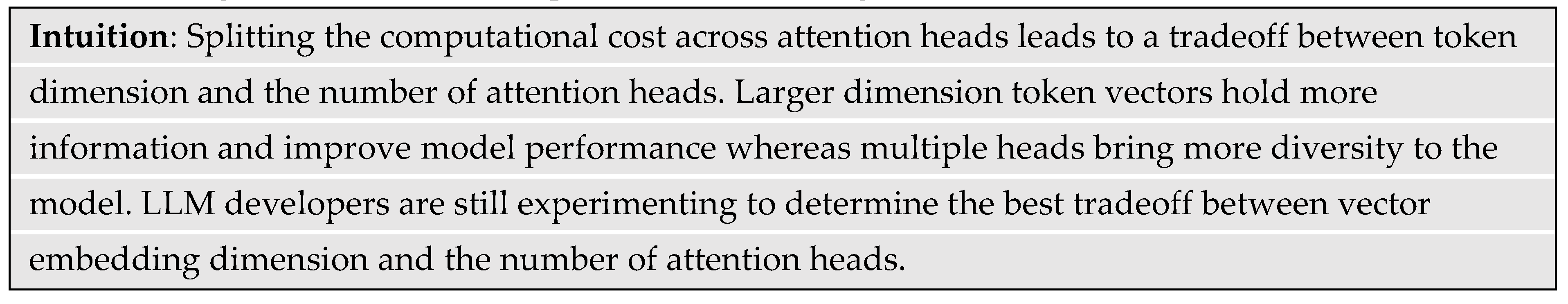
The GPT-3 implementation of attention heads maps the Q-K-V representation vectors to a lower dimension so that the computational cost for the combined heads would be equivalent to that for a single head of the full dimension. GPT-3 reduced the dimension of each head from 12,288 to 12,288/96 = 128. A learned linear network converted the concatenation of matrices from all the attention heads back to a single contextualized output matrix of the original dimension.
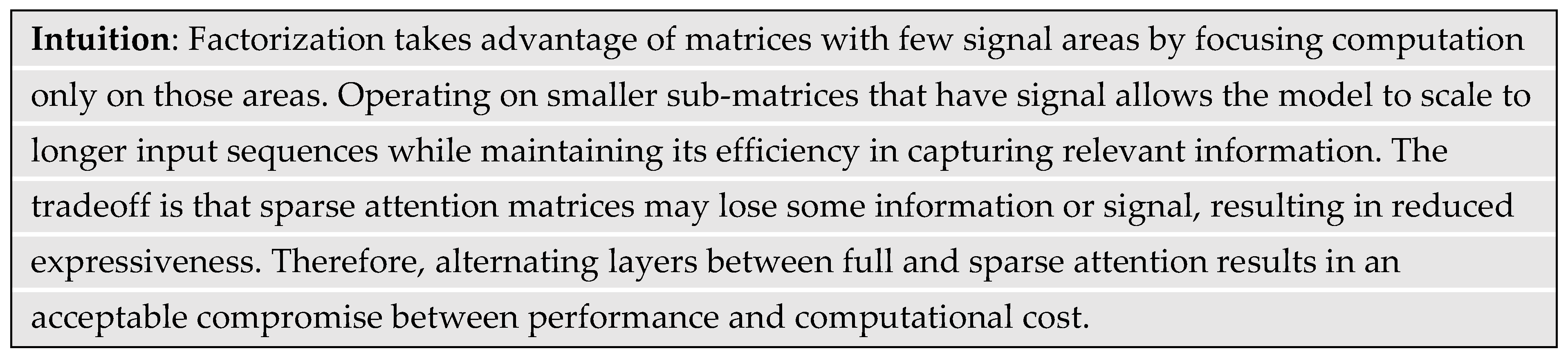
3.3. Sparse Attention
The computation cost to generate co-relevance scores is quadratic in sequence length. However, some co-relevance matrices can be sparse where large partitions of it contain zero co-relevance. Consequently, techniques emerged to reduce computational cost and memory requirements to process sparse co-relevance matrices by focusing computations only on submatrices that have co-relevance (Child, Gray, Radford, & Sutskever, 2019). The GPT-3 architecture differs slightly from the previous version in that the decoder layers alternated between dense and sparse co-relevance matrix factorization (Brown, et al., 2020). The factorization technique splits the original co-relevance matrix into smaller sub-matrices that have proportionally less non-zero elements. Hence, factorized matrices will operate on nearby tokens that have stronger co-relevance.
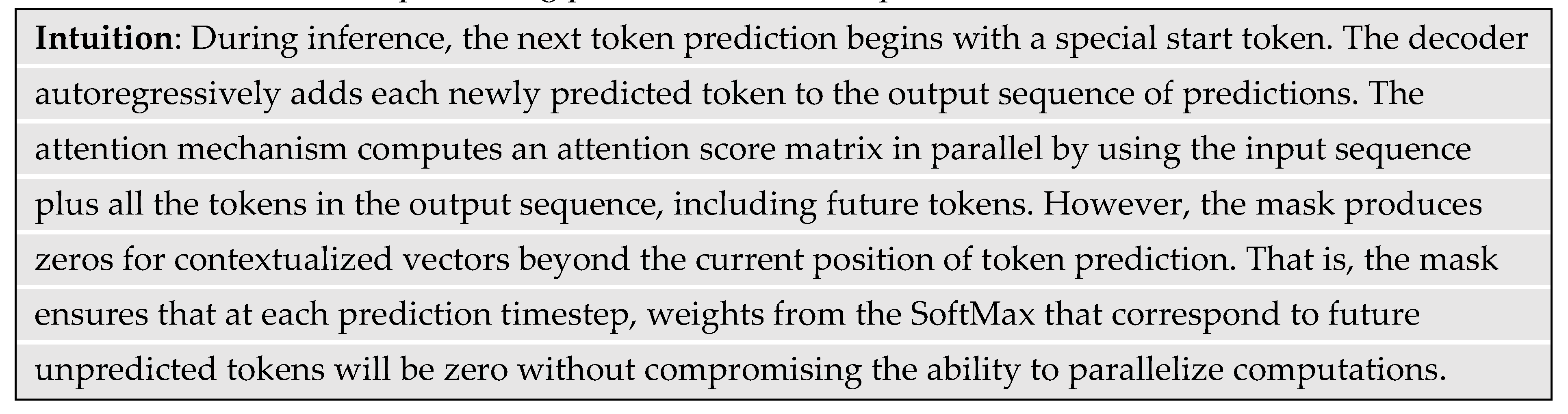
3.4. Masked Self-Attention
Self-supervised training requires that the model hide or mask future words in the training sequence prior to their prediction. The mask is a square matrix containing “1” on and below the main diagonal, and negative infinity above the diagonal. Figure 18 shows an example of the mask matrix.
Elementwise multiplication of the mask matrix with the co-relevance score matrix produces large negative numbers in the upper diagonal. This way, the SoftMax function converts the large negative numbers to near zero so that the model cannot include tokens after the current position of prediction. That is, the mask prevents the decoder from computing contextualized value vectors for future tokens while still permitting parallelized matrix operations.
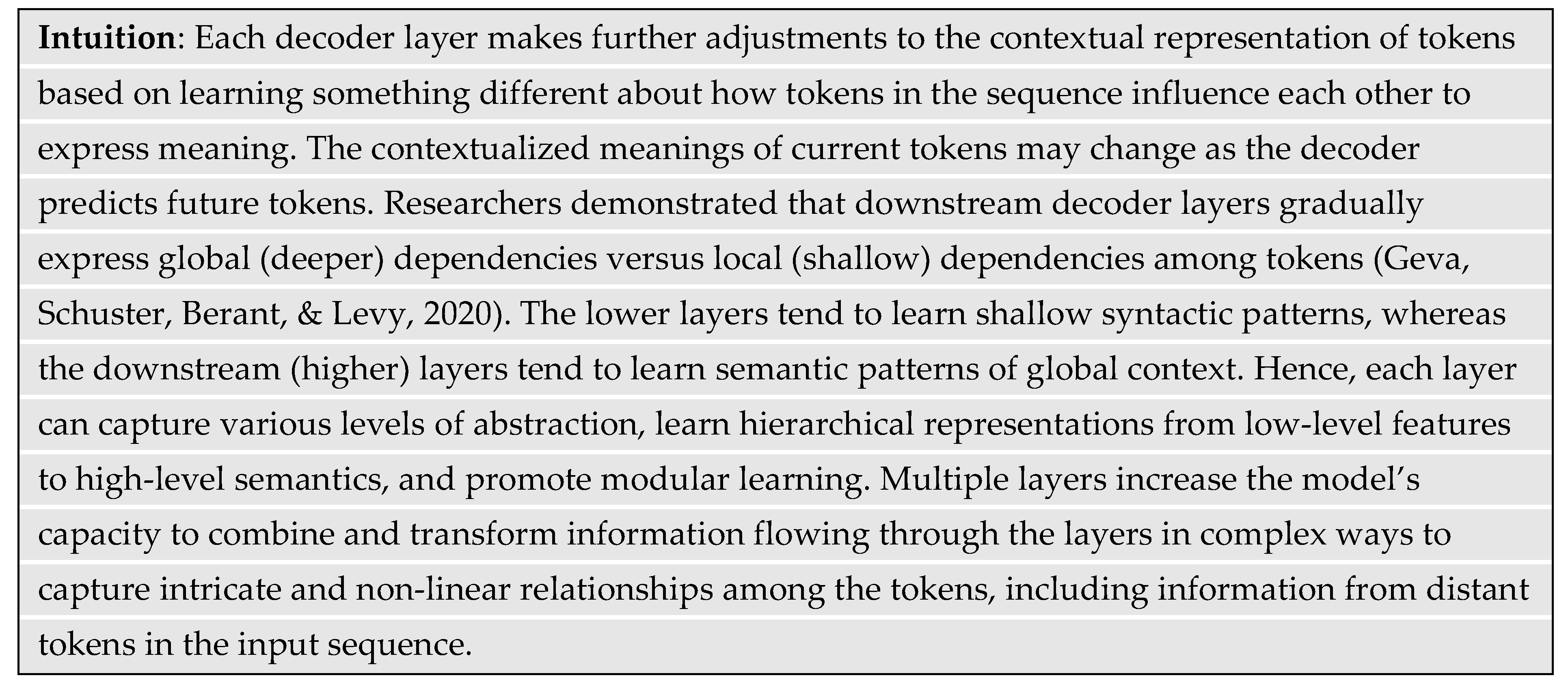
3.5. Decoder Levels
The GPT-3 architecture uses more than one decoder layer. GPT-3 uses N = 96 layers, which is the same as the number of attention heads per layer (Brown, et al., 2020). As illustrated in Figure 16, the structure of each decoder in the stack is identical. Hence, the GPT-3 architecture is effectively as wide as it is deep in computational elements. As with the number of attention heads, the number of decoder layers is a hyperparameter. Too few layers can diminish a model’s capacity for learning complex rules but too many layers can increase the risk of overfitting, which spoils the model’s ability to generalize.
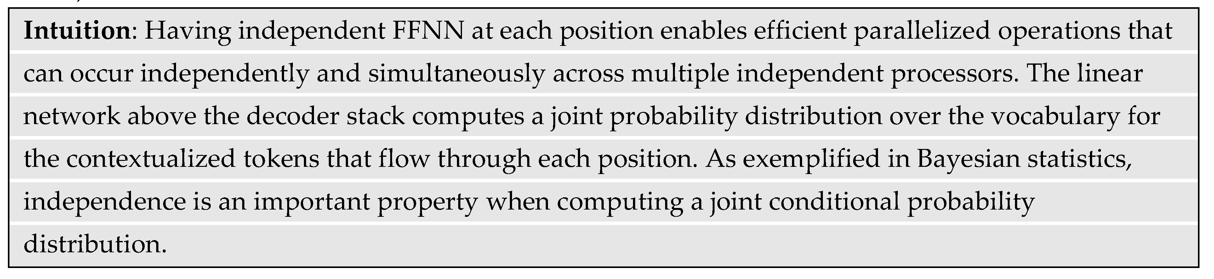
3.6. Feed Forward Neural Network
Each position of the input context window has an identical but independent and fully connected FFNN. Each FFNN of the GPT-3 architecture uses two hidden layers, each with four times the number of nodes as there are dimensions of the input vectors. Hence, the GPT-3 architecture has 4 × 12,288 = 49,152 nodes in each of the two hidden layers (Brown, et al., 2020). Research found that the FFNN accounts for two-thirds of the model parameters (Geva, Schuster, Berant, & Levy, 2020). Using the same FFNN at each position simplifies the model architecture and reduces the risk of overfitting. The independent FFNN at each position learns to continuously adjust the contextualized vector and influences how the linear networks below it learns to produce the Q-K-V projection matrices and the linear network to maximize the accuracy of the next token prediction.
The FFNN at each token position also behaves like a memory element that learns how the contextualization of tokens at that position results in the expression of both local and global semantic relationships. The memory element learns to capture local information, non-linear interactions, and patterns among tokens that appear at that position. The underlying syntactic and semantic rules of a language govern the probability that specific words will appear at specific positions, and those statistics are language dependent. For example, sentences often begin with subjects ("I," "you," "he," "she," "it," "we," "they") or proper nouns such the names of people or places (Manning & Schutze, 1999).
3.7. Linear Output Layer
The linear output layer converts each of the final contextualized tokens in the output matrix Z to probability distributions Y over the fixed vocabulary. The output matrix for a single training batch has the dimensions (sequence length × vocabulary size) = (n × m). Each vector in the output sequence contains a set of m logit values representing the probability distribution of that token over the entire vocabulary. The logit value in each position of the vector corresponds to the probability that the predicted token is the one at that position in the vocabulary.
The linear layer shares network parameters with the input word embedding network. Sharing parameters achieves token lookup consistency and memory savings. The probability distribution for the predicted token depends conditionally on the joint probability distribution of the contextualized tokens at prior positions. Experiments revealed that the probability distribution for the set of predicted tokens follows a power law decay that is characteristic of general language statistics where the nth most frequent word occurs with a frequency of 1/n (Wolfram, 2002). Therefore, only a few words will rank highest in probability. As discussed earlier, the “temperature” hyperparameter determines the token selection based on its next token probability rank. A SoftMax function that follows normalizes the logit values to positive numbers that sum to unity, which also directly ranks the probabilities.
During training, the loss function is the difference between the probability vector and the OHE vector that represents the correct target token in the vocabulary. The error is simply a difference between the OHE vector and the probability distribution for the predicted token.
4. Training Methods
The next subsections describe the three stages used to train an LLM. The first stage uses a self-supervised method, the second uses a supervised fine-tuning method, and the third stage uses reinforcement learning with human feedback to train a rewards model.
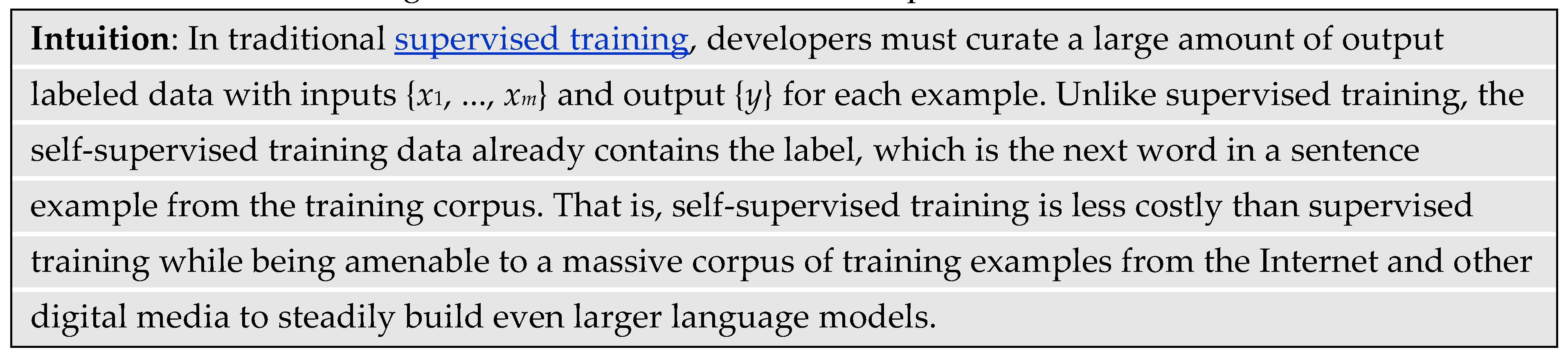
4.1. Self-Supervised Learning
Research found that the LLM’s ability to follow human instructions increases as the training data and model size increases (Bubeck, et al., 2023). The self-supervised learning of LLMs used a massive text corpus from the Internet and other places. Sources included books, Wikipedia, periodicals, and high-ranking websites. GPT-3 trained on corpus that collectively contained three hundred billion tokens (Brown, et al., 2020). Lambda Labs hypothesized that, based on the model size, GPT-3 trained for “a few weeks” on several thousand GPUs in parallel, with the equivalent being 355 years on a single state-of-the-art 28 TFLOP GPU in 2020 (Li, 2020). One TFLOP is one trillion floating-point operations per second.
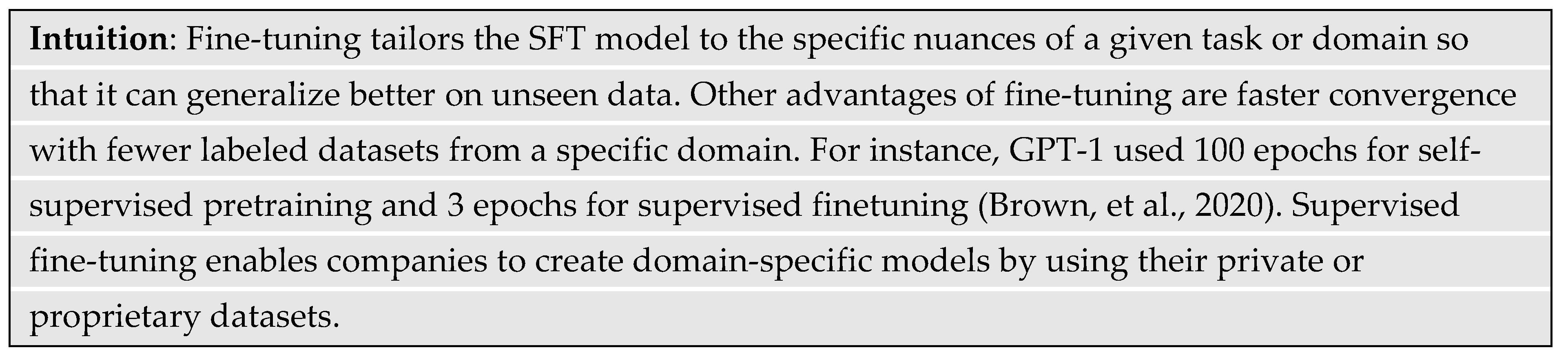
4.2. Fine-Tuning
Although the pretrained model learned natural language, it does not necessarily have the skills to generalize on specific tasks. Common examples of specific tasks are sentiment classification, text generation, text summarization, question answering, language translation, and code generation. Fine-tuning is a method to “transfer” the knowledge from a pre-trained model by adapting it to a specific task or domain. Fine-tuning uses supervised learning based on datasets labeled by humans. Such datasets demonstrate desired behavior and responses for various tasks or instructions. The dataset C used to train a supervised fine-tuned (SFT) model has token sequences [x1, ..., xm] and the desired output labels y. The developers modify the pretrained model by adding another linear layer with parameters Wy to the output hlm of the last decoder. Hence, the transformation performed is [hlm][Wy]. The model then learns the parameters of Wy by training it with each instance of the entire labeled dataset C. After training, the SoftMax produces the probability of a label y given an unseen input sequence [x1, ..., xm]. Hence, the SFT learned to maximize the following objective function over all instances {[x1, ..., xm], y} in the labeled training dataset C (Radford, Narasimhan, Salimans, & Sutskever, 2018):
4.3. Reinforcement Learning
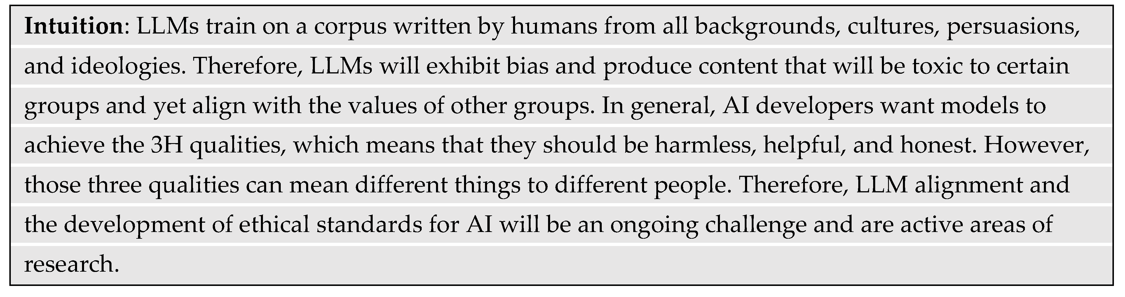
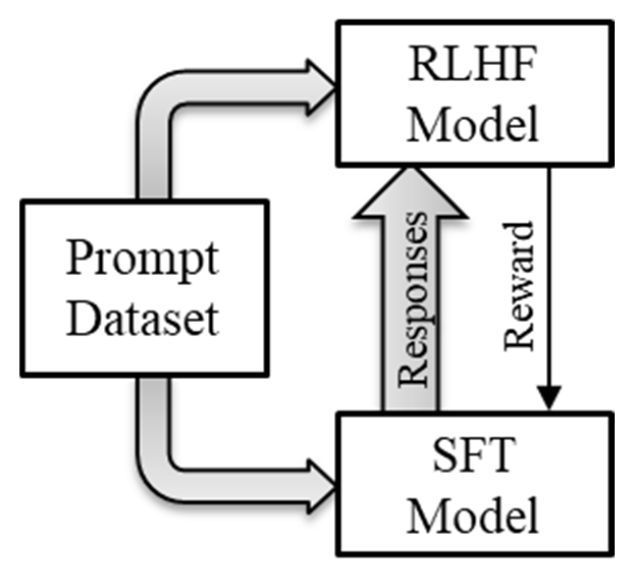
SFT language models have a limited ability to align with user intentions. Their responses could lack helpfulness, contain inaccurate facts, lack interpretability, and include toxic, offensive, or harmful content. To address that problem, ChatGPT developers used a reinforcement learning (RL) technique to augment the SFT model. The RL method helped the SFT model learn a “policy” to better align it with human intentions. The technique first used human feedback to train a separate “rewards” model. The reinforcement learning with human feedback (RLHF) method trained the rewards model to produce a scalar rewards output based on a series of responses from the SFT model to a prompt (Ouyang, et al., 2022). The RLHF technique required human labelers to rank four to nine responses from the SFT model to a single prompt. To simplify the ranking task, human labelers ranked pairs of responses separately, for all unique combinations of responses, based on their quality or appropriateness for a given task or instruction. The prompt and the batch of pairwise ranked responses became the training data for the rewards model. Figure 19 illustrates how the trained model from RLHF then trains the SFT model for alignment.
SFT language models have a limited ability to align with user intentions. Their responses could lack helpfulness, contain inaccurate facts, lack interpretability, and include toxic, offensive, or harmful content. To address that problem, ChatGPT developers used a reinforcement learning (RL) technique to augment the SFT model. The RL method helped the SFT model learn a “policy” to better align it with human intentions. The technique first used human feedback to train a separate “rewards” model. The reinforcement learning with human feedback (RLHF) method trained the rewards model to produce a scalar rewards output based on a series of responses from the SFT model to a prompt (Ouyang, et al., 2022). The RLHF technique required human labelers to rank four to nine responses from the SFT model to a single prompt. To simplify the ranking task, human labelers ranked pairs of responses separately, for all unique combinations of responses, based on their quality or appropriateness for a given task or instruction. The prompt and the batch of pairwise ranked responses became the training data for the rewards model. Figure 19 illustrates how the trained model from RLHF then trains the SFT model for alignment.
The trained rewards model automatically generates a scalar reward to further train the SFT model to improve its alignment with preferences of the human trainer. The RL method included the reward in the backpropagation during training. In this way, the SFT model developed policies to maximize its cumulative reward over time. ChatGPT used a method called proximal policy optimization (PPO) to ensure that the model does not overfit to rewards. That is, PPO assured that the new policies created did not deviate much from the original learned capabilities of the SFT model that enabled it to generalize on unseen data (Ouyang, et al., 2022).
Broadly, model alignment refers to the ability of AI models to align with user intentions. However, “user intentions” can be varied and conflicting. The capabilities of LLMs to blur the distinction between human- and AI-generated content has raised concerns about misinformation, manipulation, and misuse. Examples include perpetuating stereotypes, discrimination, or offensive content, sharing confidential information, generating fake news, propagating computer viruses, and teaching perpetrators how to easily harm people while evading discovery (Schaul, Chen, & Tiku, 2023).
5. Conclusions
The proliferation of data on the Internet combined with the exponential growth in computing capacity and the discovery of a more capable language model architecture led to a tipping point in the performance of AI chatbots. This primer provided a comprehensive and accessible tutorial on large language models (LLMs) such as ChatGPT and Google’s Bard. The goal was to demystify their underlying theory, architecture, and methods for a broad audience. The primer provided insights into key computing elements, architectural choices, and state-of-the-art training methods that have enabled these models to achieve groundbreaking performance. Prompt engineering is an emerging skill that users will need to achieve effective interaction with a computer through natural language. This new way of human-computer interaction has significantly increased the accessibility of computers, which will pave the way for an explosion of novel applications across various domains. With continued advancements in LLM capability, it is crucial for researchers, developers, and users to understand their inner workings. The future discovery of more efficient architectures, the development of dedicated neural network microchips, and the emergence of AI models that can train even more powerful AI models will lead to ever-scaling advancements. Hence, fostering a broader understanding of LLMs will contribute to responsible innovation and informed discussions on their potential impact on society, ensuring that humans harness the technology for greater good while eliminating unintended negative consequences.
6. Future Work
Readers at the time of this writing will remember using a deck of “punch cards” to program computers through the 1980s. Since then, low-level computer languages, like assembly language, replaced punch cards. Later higher-level programming languages like Basic, C, Java, and Python replaced assembly language. The human-machine interface also switched from in-line typing (e.g., disk operating system) to a graphical user’s interface (GUI) with application icons. At the time of this writing, humanity has entered a new era of human-machine interface where users can use natural language to instruct computers. This capability has increased the accessibility of computers to a much larger population.
Continued accessibility enhancement will result in an explosion of new applications across all domains. For example, users can do simple tasks like asking for recipes that use a finite set of ingredients to more complex tasks such as data mining a biological dataset to discover a cure for a disease. However, there are various levels of prompting complexity that can have an enormous effect on the quality and helpfulness of the responses from the AI chatbot. The familiar adage “garbage in, garbage out” still holds.
Prompt engineering has emerged as a new skill to appropriately prompt LLMs to produce desired results. Good prompts will have four parts: Context setting, specific instructions, format/structure, and optional examples.
- Context setting provides a brief background about the topic or task. This guides the AI into an internal state for understanding the context for which it should generate a response. That is, LLMs rely on the information provided in the prompt to understand the topic for generating meaningful and relevant responses.
- Specific instructions clearly state the requirements, questions, or tasks without any ambiguity. This focuses the LLM to reduce changes of generating irrelevant or off-topic responses.
- Format/structure tells the LLM the format or sentence structure to produce the response. This includes word count, bullet points, and headings of an outline. The AI can also produce output in tabular form or indirectly generate graphics in HTML using scalar vector graphics (SVG) that a browser can render.
- Examples providing the LLM with desired outputs helps it better understand the style, format, or output sought. The results improve with one or more examples. The literature refers to providing zero, one, or more examples as zero-shot, one-shot, or few-shot prompting, respectively.
Research posited that “chain-of-thought” prompting elicits “reasoning” in LLMs (Wei, et al., 2023). No doubt, discoveries of new prompting “hacks” will follow. Prompt engineering has emerged as a new sought-after skill and dozens of books are already available on the subject. Future work will examine approaches towards achieving AGI, which may require innovations that go beyond simply continuing to increase the model size and training data.
Declarations: The author has no conflicts of interest to declare. The author created all the figures in this primer. The author did not use AI tools to generate any portion of this document. Human peers suggested edits to the original manuscript, for which the author is grateful.
References
- Ba, J. L., Kiros, J. R., & Hinton, G. E. (2016). Layer normalization. arXiv:1607.06450v1 [stat.ML]. arXiv:1607.06450v1 [stat.ML]. [CrossRef]
- Bahdanau, D., Cho, K., & Bengio, Y. (2014). Neural machine translation by jointly learning to align and translate. 3rd International Conference on Learning Representations (ICLR 2015). San Diego, CA, USA: arXiv:1409.0473v7. arXiv:1409.0473v7. [CrossRef]
- Bengio, Y., Ducharme, R., & Vincent, P. (2000). A Neural Probabilistic Language Model. In T. K. Leen, T. G. Dietterich, & V. Tresp (Ed.), Advances in Neural Information Processing Systems 13 (NIPS 2000). The MIT Press. Retrieved from https://mitpress.mit.edu/9780262526517/advances-in-neural-information-processing-systems-13/.
- Bridgelall, R. (2022). Tutorial On Support Vector Machines. Research Square. [CrossRef]
- Brown, T. B. , Mann, B., Ryder, N., Subbiah, M., Kaplan, J., Dhariwal, P.,... Amodei, D. (2020). Language Models are Few-Shot Learners. arXiv:2005.14165v4 [cs.CL], arXiv:2005.14165v4 [cs.CL]. [CrossRef]
- Bubeck, S. , Chandrasekaran, V., Eldan, R., Gehrke, J., Horvitz, E., Kamar, E.,... Zhang, Y. (2023). Sparks of Artificial General Intelligence: Early experiments with GPT-4. arXiv:2303.12712v4 [cs.CL], arXiv:2303.12712v4 [cs.CL]. [CrossRef]
- Child, R. , Gray, S., Radford, A., & Sutskever, I. (2019). Generating long sequences with sparse transformers. arXiv:1904.10509v1 [cs.LG], arXiv:1904.10509v1 [cs.LG]. [CrossRef]
- Chomsky, N., Roberts, I., & Watumull, J. (2023, March 8). Noam Chomsky: The False Promise of ChatGPT. The New York Times. Retrieved from https://www.nytimes.com/2023/03/08/opinion/noam-chomsky-chatgpt-ai.html.
- Géron, A. (2019). Hands-on Machine Learning with Scikit-Learn, Keras, and TensorFlow: Concepts, Tools, and Techniques to Build Intelligent Systems (2nd ed.). Sebastopol, California: O'Reilly Media.
- Geva, M. , Schuster, R., Berant, J., & Levy, O. (2020). Transformer feed-forward layers are key-value memories. arXiv:2012.14913v2 [cs.CL], arXiv:2012.14913v2 [cs.CL]. [CrossRef]
- He, K., Zhang, X., Ren, S., & Sun, J. (2016). Deep Residual Learning for Image Recognition. 2016 IEEE Conference on Computer Vision and Pattern Recognition (CVPR) (pp. 770-778). Las Vegas, NV, USA: IEEE. [CrossRef]
- Hendrycks, D. , & Gimpel, K. (2016). Gaussian Error Linear Units (GELUs). arXiv:1606.08415v4 [cs.LG], arXiv:1606.08415v4 [cs.LG]. [CrossRef]
- Hornik, K., Stinchcombe, M., & White, H. (1989). Multilayer feedforward networks are universal approximators. Neural networks, 2(5), 359-366. [CrossRef]
- Krizhevsky, A., Sutskever, I., & Hinton, G. E. (2017). Imagenet classification with deep convolutional neural networks. Communications of the ACM, 60(6), 84-90. 6. [CrossRef]
- Li, C. (2020, June 3). OpenAI's GPT-3 Language Model: A Technical Overview. Retrieved from Lambda: https://lambdalabs.com/blog/demystifying-gpt-3.
- Liu, Y. , Han, T., Ma, S., Zhang, J., Yang, Y., Tian, J.,... Ge, B. (2023). Summary of ChatGPT/GPT-4 research and perspective towards the future of large language models. arXiv:2304.01852v2 [cs.CL], arXiv:2304.01852v2 [cs.CL]. [CrossRef]
- Manning, C., & Schutze, H. (1999). Foundations of Statistical Natural Language Processing. Cambridge, Massachusetts, USA: MIT Press.
- Otter, D. W., Medina, J. R., & Kalita, J. K. (2020). A survey of the usages of deep learning for natural language processing. IEEE transactions on neural networks and learning systems, 32(2), 604-624. 2. [CrossRef]
- Ouyang, L. , Wu, J., Jiang, X., Almeida, D., Wainwright, C., Mishkin, P.,... Lowe, R. (2022). Training language models to follow instructions with human feedback. In S. Koyejo, S. Mohamed, A. Agarwal, D. Belgrave, K. Cho, & A. Oh (Ed.), Advances in Neural Information Processing Systems 35 (NeurIPS 2022). 35, pp. 27730-27744. Curran Associates, Inc. Retrieved from https://proceedings.neurips.cc/paper_files/paper/2022. 2022. [Google Scholar]
- Peters, J. (2023, March 14). The Bing AI bot has been secretly running GPT-4. The Verge Retrieved from https://www.theverge.com/2023/3/14/23639928/microsoft-bing-chatbot-ai-gpt-4-llm.
- Radford, A., Narasimhan, K., Salimans, T., & Sutskever, I. (2018). Improving Language Understanding by Generative Pre-Training. San Francisco, California: OpenAI. Retrieved from https://github.com/openai/finetune-transformer-lm.
- Roose, K. (2022, December 5). The Brilliance and Weirdness of ChatGPT. The New York Times. Retrieved from https://www.nytimes.com/2022/12/05/technology/chatgpt-ai-twitter.html.
- Schaul, K., Chen, S. Y., & Tiku, N. (2023, April 19). Inside the secret list of websites that make AI like ChatGPT sound smart. The Washington Post. Retrieved April 19, 2023, from https://www.washingtonpost.com/technology/interactive/2023/ai-chatbot-learning/.
- Sennrich, R. , Haddow, B., & Birch, A. (2015). Neural machine translation of rare words with subword units. arXiv:1508.07909v5 [cs.CL], arXiv:1508.07909v5 [cs.CL]. [CrossRef]
- Stevenson, A. (Ed.). (2010). Oxford dictionary of English. USA: Oxford University Press.
- Tobler, W. R. (1970). A computer movie simulating urban growth in the Detroit region. Economic geography, 46(sup1), 234-240. [CrossRef]
- Vaswani, A. , Shazeer, N., Parmar, N., Uszkoreit, J., Jones, L., Gomez, A. N.,... Polosukhin, I. (2017). Attention is all you need. In I. Guyon, U. V. Luxburg, S. Bengio, H. Wallach, R. Fergus, S. Vishwanathan, & R. Garnett (Ed.), Advances in neural information processing systems 30 (NIPS 2017). Retrieved from https://proceedings.neurips.cc/paper_files/paper/2017. 2017. [Google Scholar]
- W3Techs. (2023, April 18). Usage of character encodings broken down by ranking. Retrieved April 18, 2023, from Web Technology Surveys (W3Techs): https://w3techs.com/technologies/cross/character_encoding/ranking.
- Walczak, S. (2019). Advanced Methodologies and Technologies in Artificial Intelligence, Computer Simulation, and Human-Computer Interaction. Hershey, Pennsylvania, USA: IGI Global. [CrossRef]
- Wei, J. , Wang, X., Schuurmans, D., Bosma, M., Ichter, B., Xia, F.,... Zhou, D. (2023). Chain-of-Thought Prompting Elicits Reasoning in Large Language Models. arXiv:2201.11903v6 [cs.CL], arXiv:2201.11903v6 [cs.CL]. [CrossRef]
- Widdowson, H. (2007). J.R. Firth, 1957, papers in linguistics 1934–51. International Journal of Applied Linguistics, 17(3), 402-413. [CrossRef]
- Wolfram, S. (2002). A New Kind of Science. Champaign, IL: Stephen Wolfram, LLC. Retrieved from https://www.wolframscience.com/nks/notes-8-8--zipfs-law/.
Figure 1.
LLM functional flow.
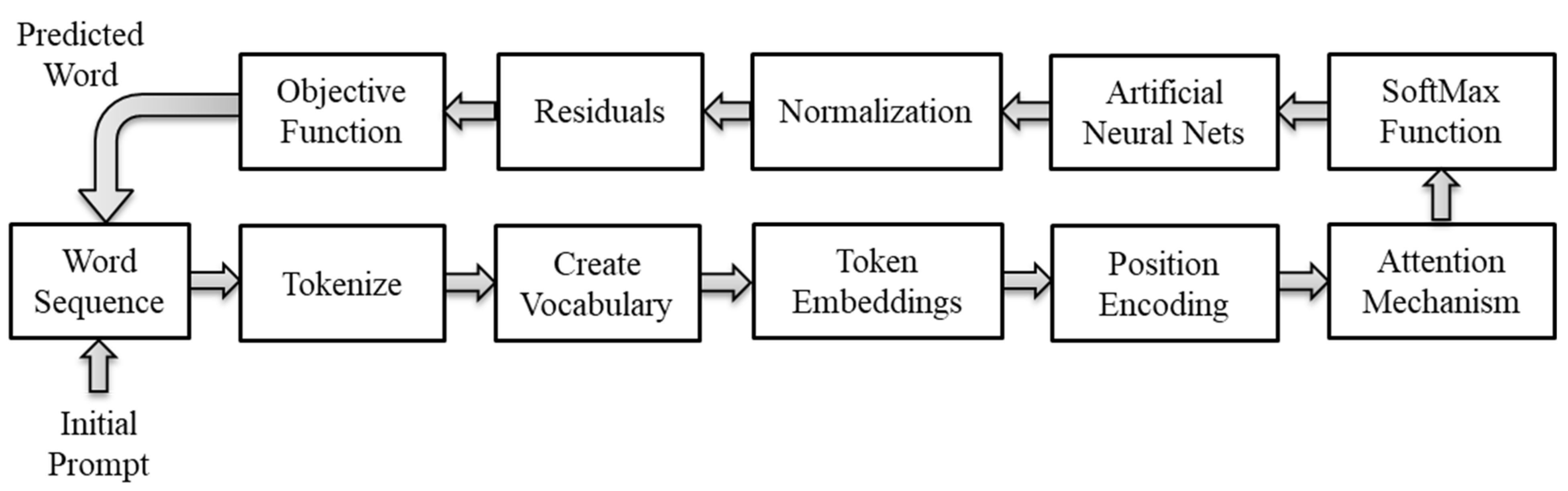
Figure 2.
Building the vocabulary for embedding.
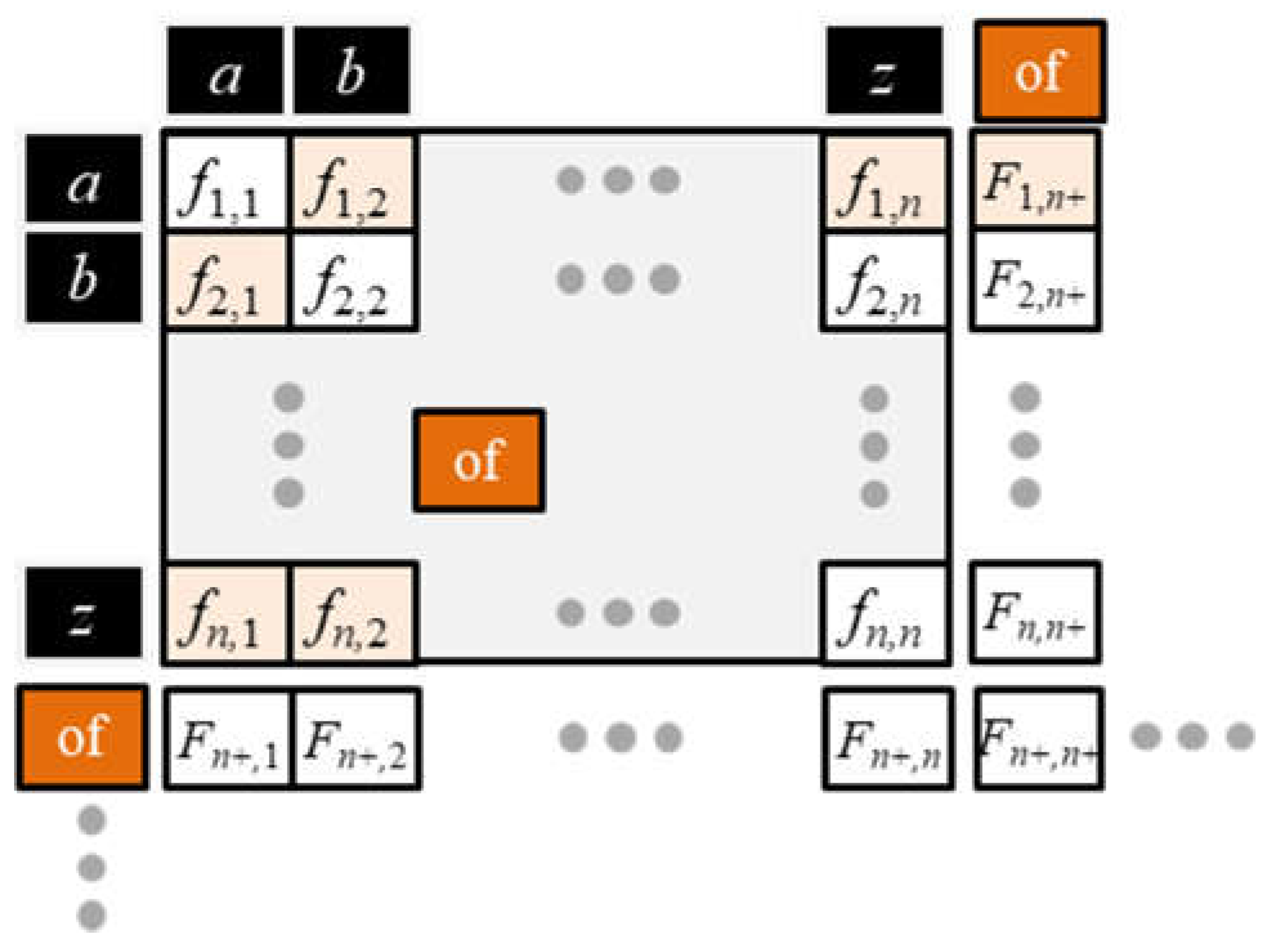
Figure 3.
Example of how a single word difference can change the context of a sentence.
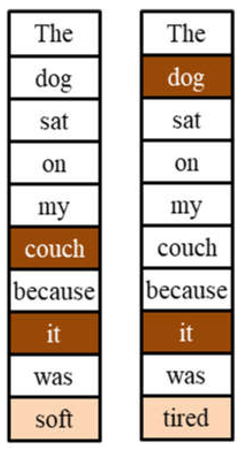
Figure 4.
Co-relevance vectors moves closer to each other in the embedding space.
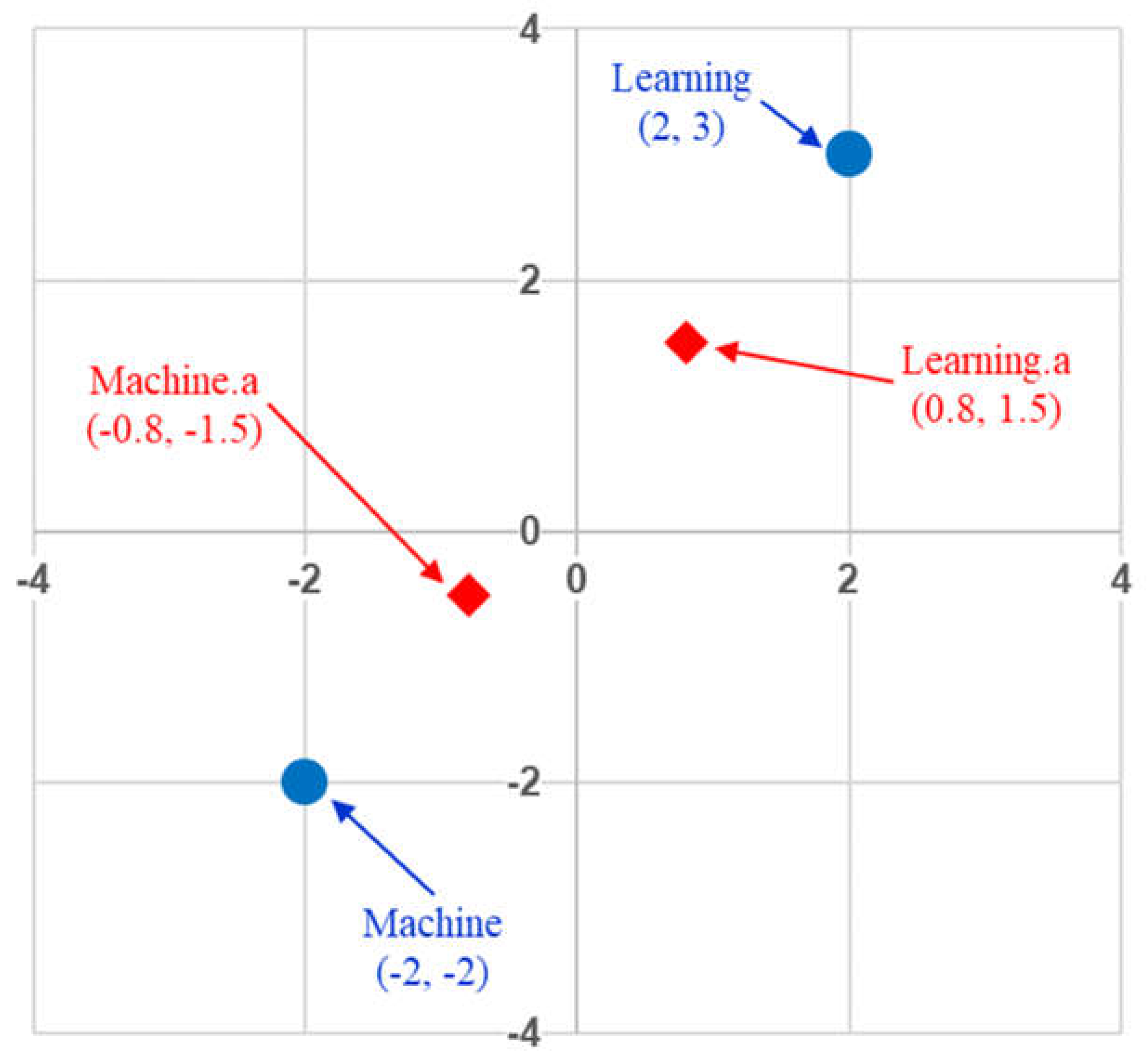
Figure 5.
Calculating the attention vectors for the input sequence.
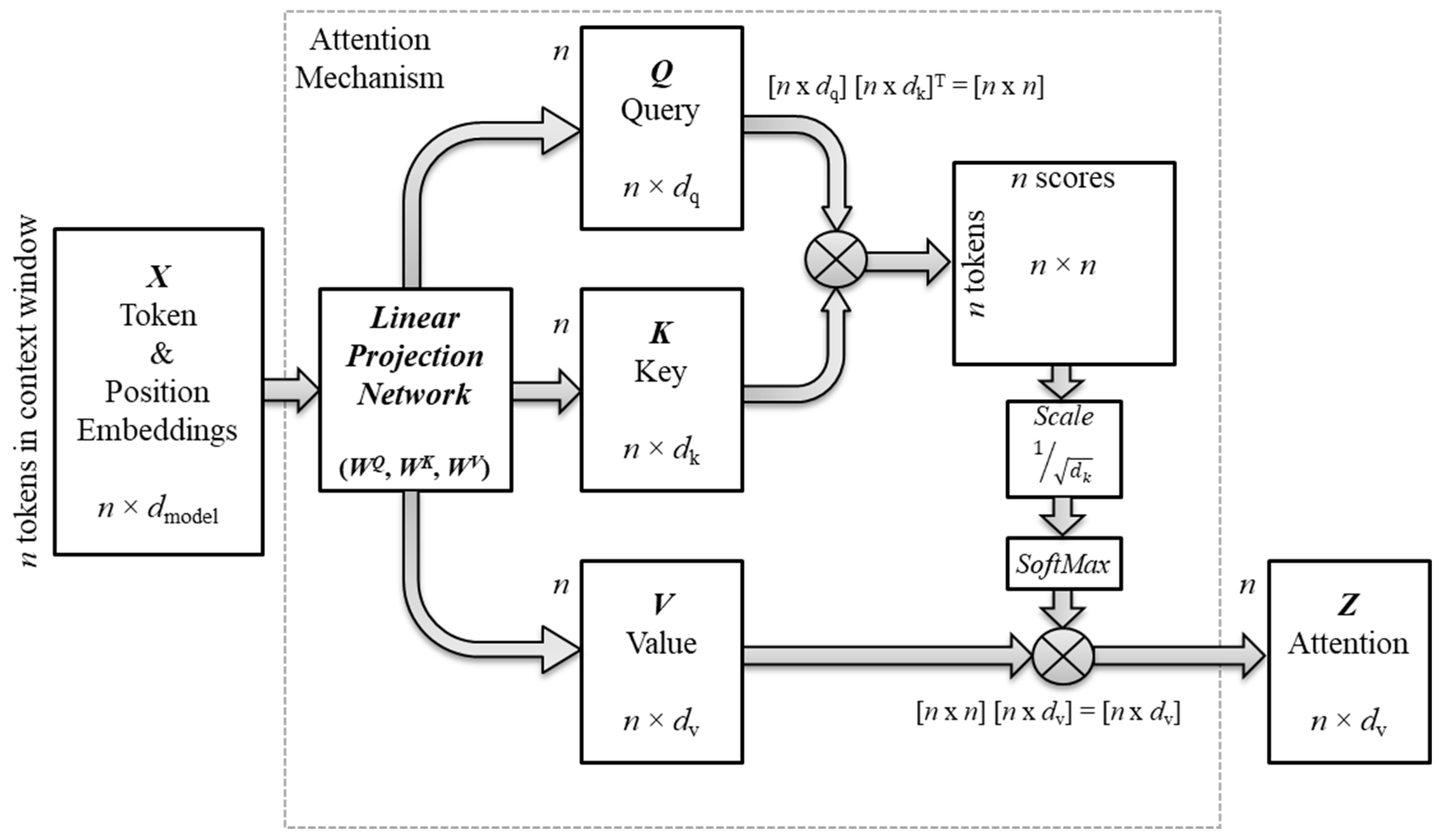
Figure 6.
Matrix multiplication is equivalent of the dot product.
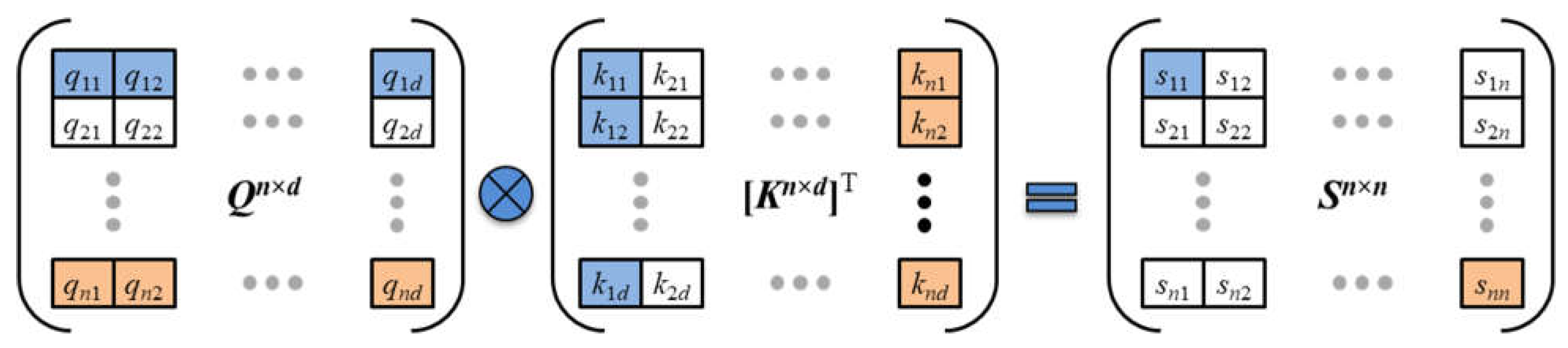
Figure 7.
Co-relevance scores are associated with every pairwise combination of tokens in the input sequence.
Figure 7.
Co-relevance scores are associated with every pairwise combination of tokens in the input sequence.
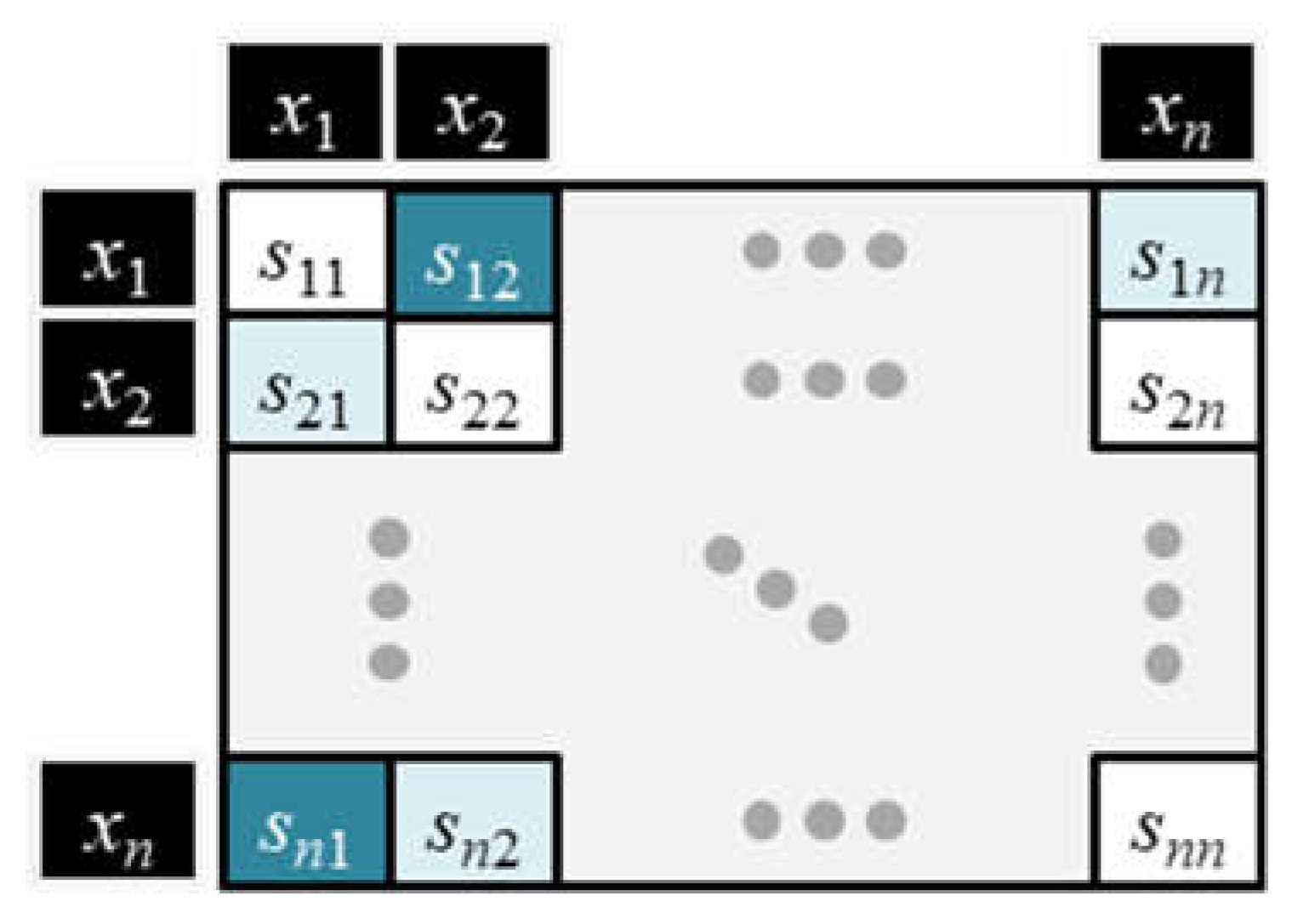
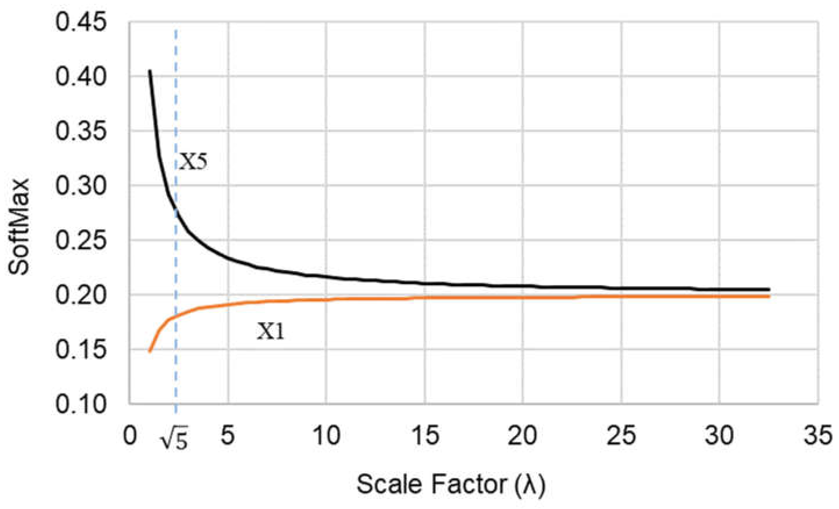
Figure 9.
ANN (2H × 2H) function approximator.
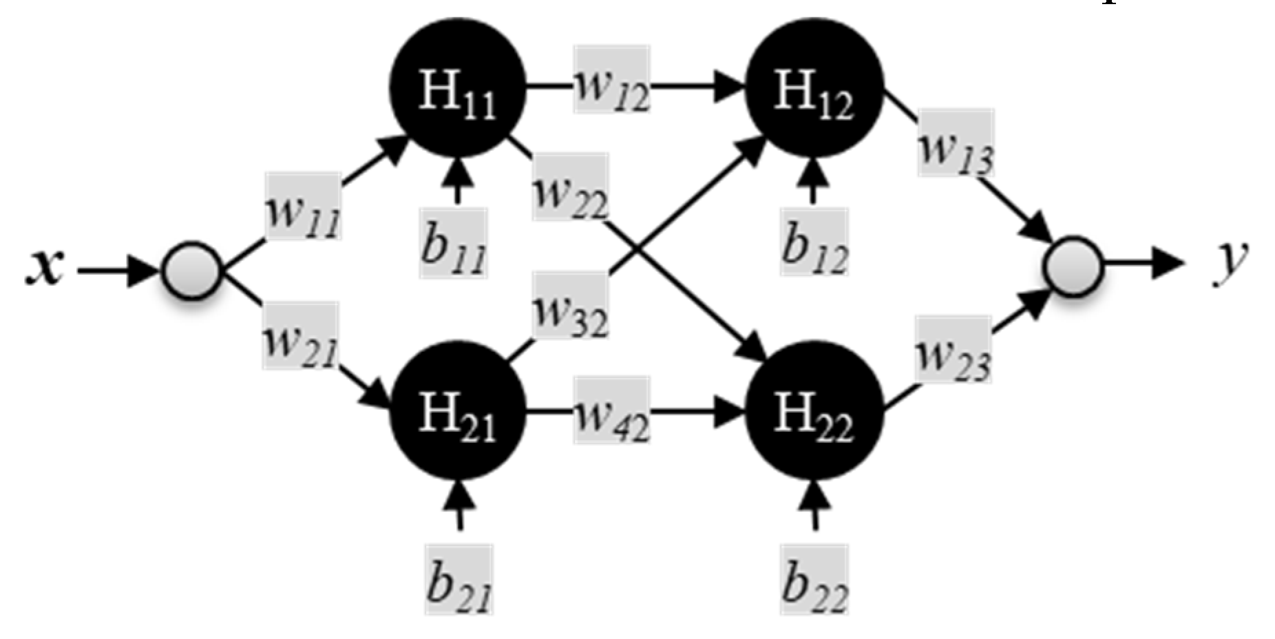
Figure 10.
Comparison of ReLU, Sigmoid, and GELU activation functions.
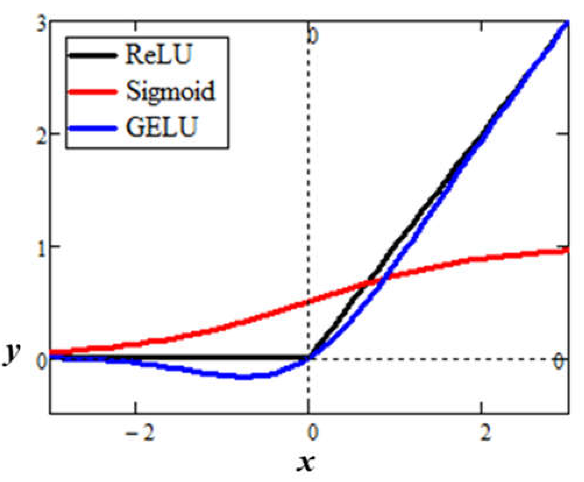
Figure 11.
ReLU activation functions with various parameters and scaling.
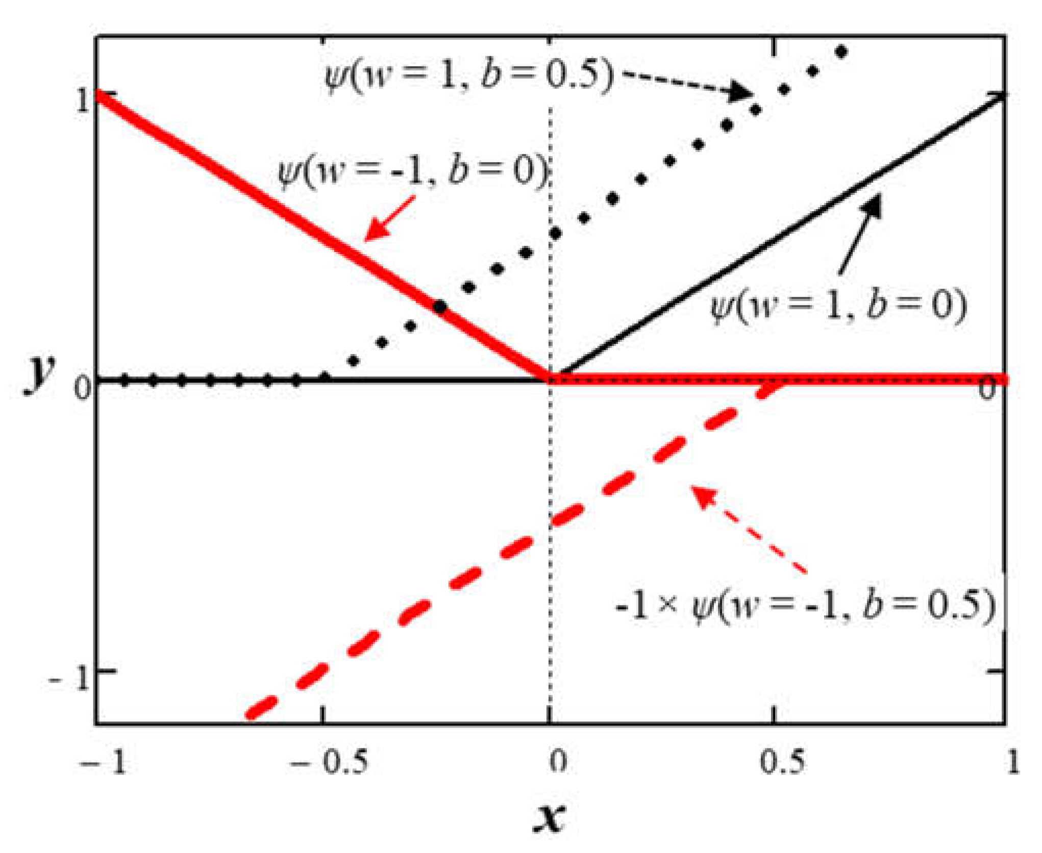
Figure 12.
Neural network with one hidden layer of three nodes with ReLU activation (1H: 3×1).
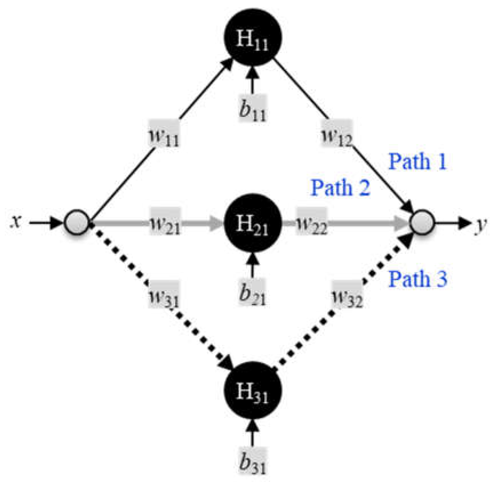
Figure 13.
ANN (1H: 3×1, ReLU) a) sinusoid estimation, and b) intermediate functions.
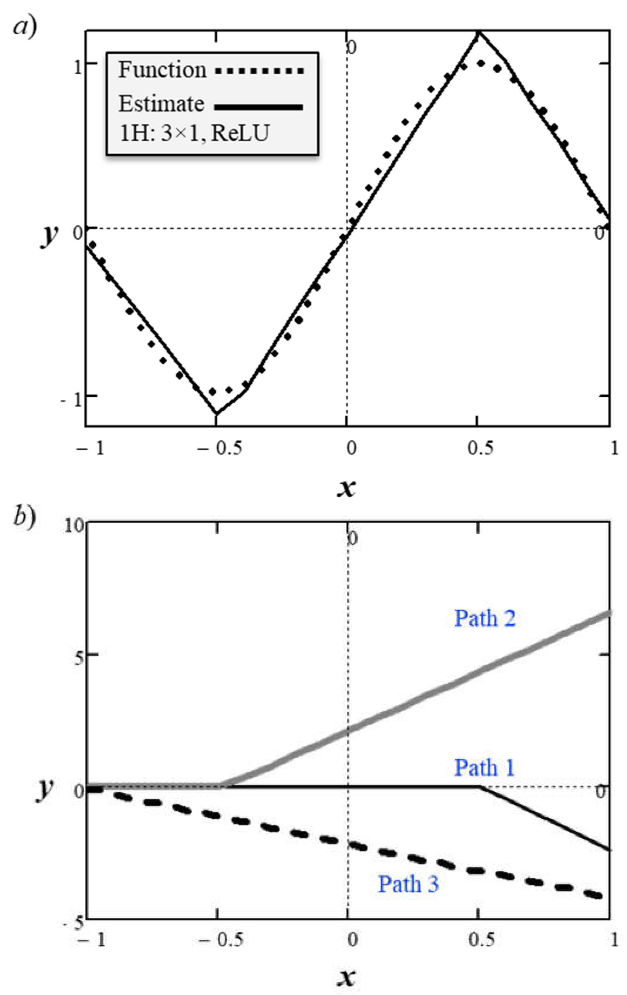
Figure 14.
ANN {1H: 6×1, ReLU} a) sinusoid estimation, and b) RMSE trend.
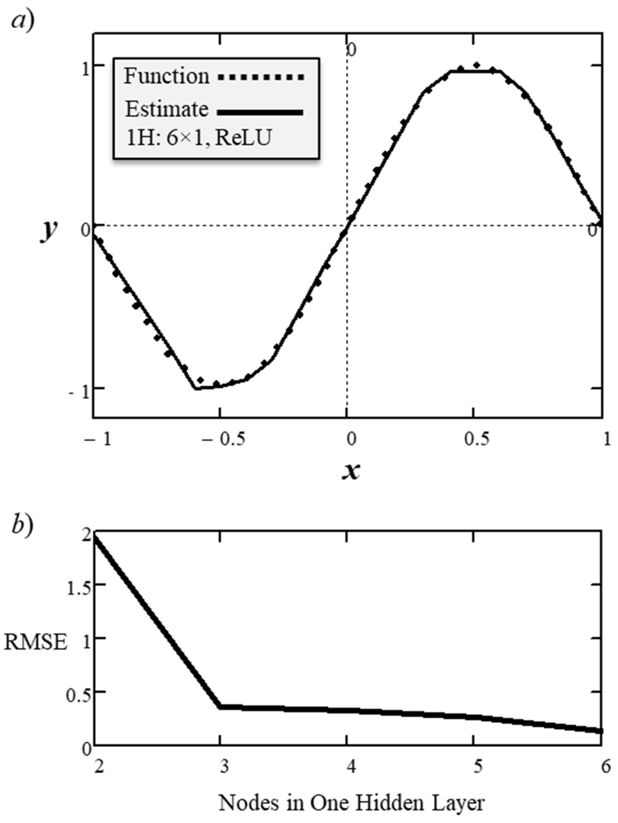
Figure 15.
Residual and standardized residual vectors maintain their relative relationship in the embedding space.
Figure 15.
Residual and standardized residual vectors maintain their relative relationship in the embedding space.
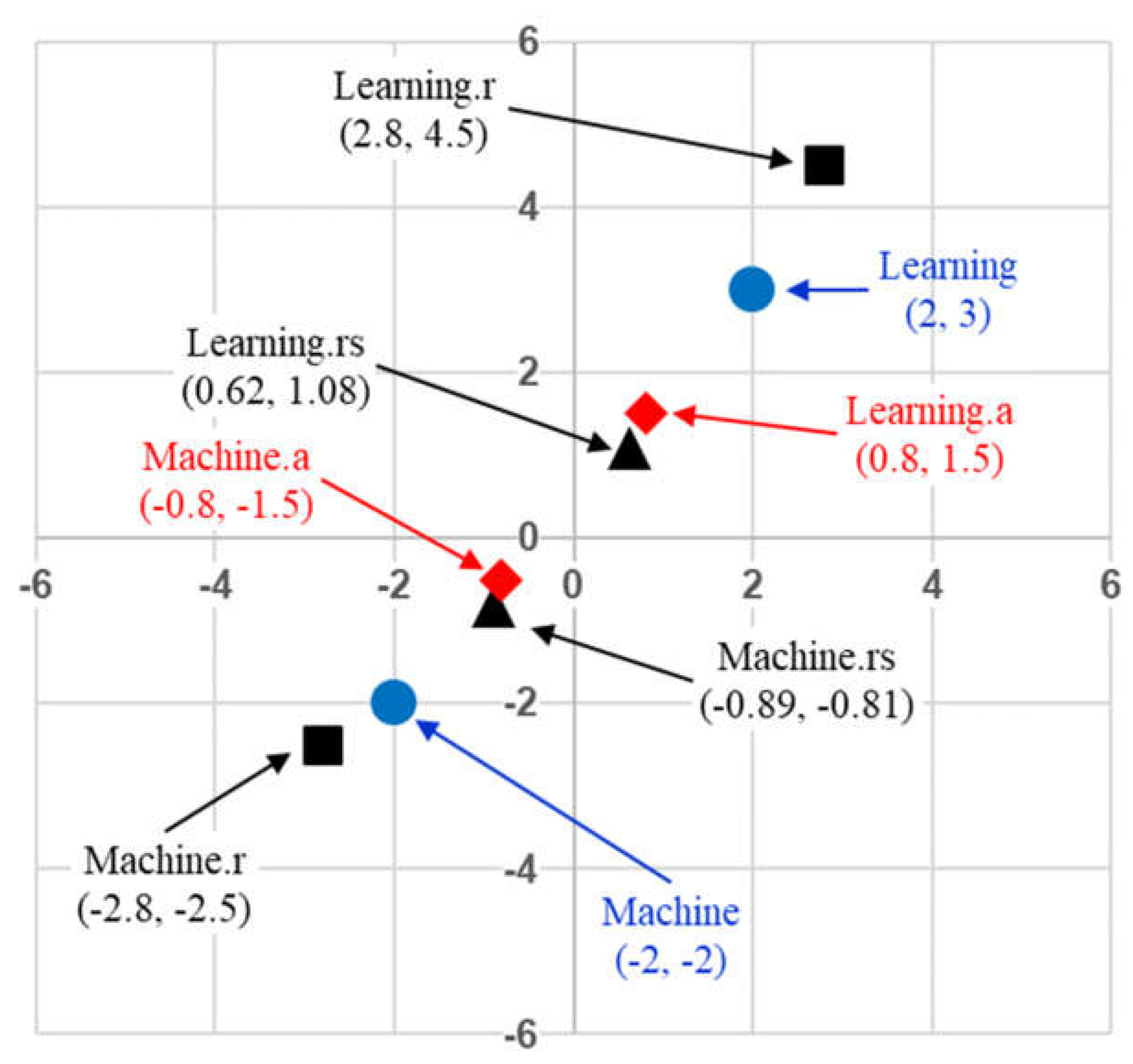
Figure 16.
Overview of the GPT architecture.
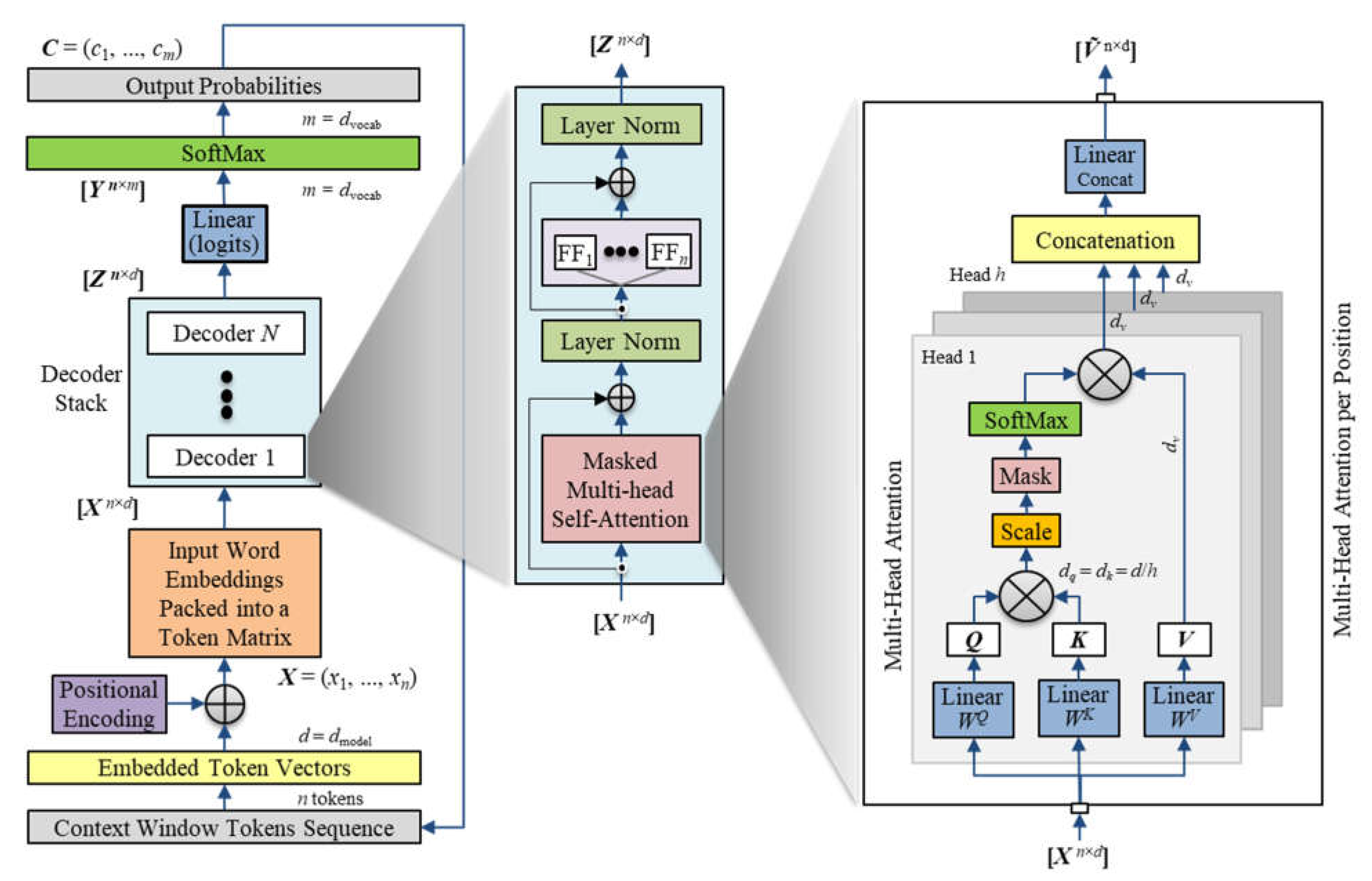
Figure 17.
Concatenation of co-relevance from different attention heads.
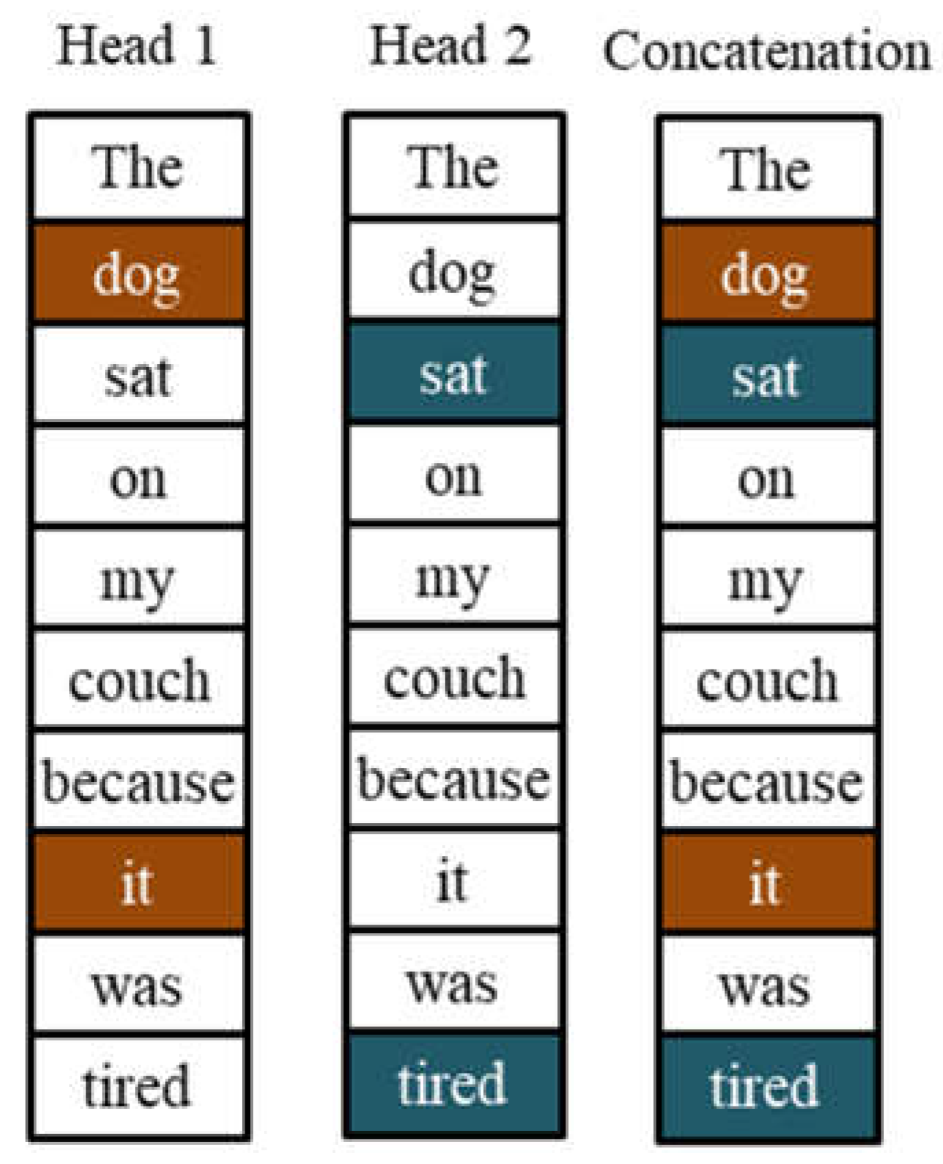
Figure 18.
Mask matrix for the attention scores.
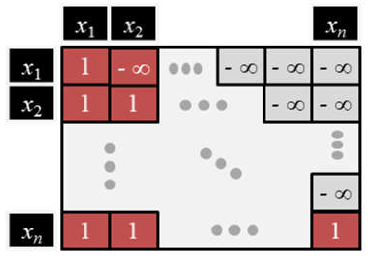
Figure 19.
Training the SFT model using RLHF.
Disclaimer/Publisher’s Note: The statements, opinions and data contained in all publications are solely those of the individual author(s) and contributor(s) and not of MDPI and/or the editor(s). MDPI and/or the editor(s) disclaim responsibility for any injury to people or property resulting from any ideas, methods, instructions or products referred to in the content. |
© 2023 by the authors. Licensee MDPI, Basel, Switzerland. This article is an open access article distributed under the terms and conditions of the Creative Commons Attribution (CC BY) license (http://creativecommons.org/licenses/by/4.0/).
Copyright: This open access article is published under a Creative Commons CC BY 4.0 license, which permit the free download, distribution, and reuse, provided that the author and preprint are cited in any reuse.


