
Submitted:
01 May 2023
Posted:
05 May 2023
You are already at the latest version
Abstract
Accurate detection and quantification of regional vegetation trends is essential for understanding the dynamics of landscape ecology and vegetation distribution. We applied a comprehensive trend analysis to satellite data to describe geo-spatial changes in vegetation along the Pacific slope of Peru and northern Chile, from sea level to the continental divide, a region characterised by biologically unique and highly sensitive arid and semi-arid environments. Our statistical analyses show broad regional patterns of positive trends in EVI, called “greening” alongside patterns of “browning” where trends are negative between 2000 and 2020. The coastal plain and foothills, up 1000m, contain notable greening of the coastal Lomas and newly irrigated agricultural lands occurring alongside browning trends related to changes in land use practices and urban development. Strikingly, the precordilleras show a distinct ’greening strip’ which extends from approximately 6°S to 22°S, with an altitudinal trend; ascending from the tropical lowlands (170-780 m) in northern Peru, to the subtropics (1000-2800 m) in central Peru, and temperate zone (2600-4300 m) in southern Peru and northern Chile. We find that the geographical characteristics of the greening strip do not match climate zones previously established by Köppen and Geiger. Greening and browning trends in the coastal deserts and the high Andes lie within well defined climatic and life zones, producing variable but identifiable trends. However, the distinct Pacific slope greening presents an unexpected distribution with respect to the regional Köppen-Geiger climate and life zones. This work provides insights on understanding the effects of climate change on Peru’s diverse ecosystems in highly sensitive, biologically rich arid and semi-arid environments on the Pacific slope.
Keywords:
MODIS
; EVI
; time series
; greening
; browning
; Andes
; Peru
; climate zones
; life zones
; trend
1. Introduction
Climatic conditions are considered to be the primary determinants of vegetation patterns, mediated by a complex of locally specific variables that significantly impact ecosystem services, from watershed protection and soil conservation to land use utility and resource availability [1,2]. The Köppen-Geiger climate classification model is based on the ambition to understand what determines the types of vegetation that could be found in any given region [3,4]. It is a widely used system that divides climates into five principal groups (tropical, arid, temperate, continental, and polar), each sub-divided according to rainfall and temperature data to give thirty discrete climate zones [3]. The Köppen-Geiger system produces geographical zones strongly linked to vegetation productivity and the geographical determinants of plant diversity, which makes it particularly useful in understanding and predicting regional changes in the distribution of life zones [2,5]. It is the dynamic character of climatic conditions that produce long-term changes in vegetative distribution [6,7,8]. This complex interaction significantly impacts environmental processes that determine ecosystem services and resource availability. Globally, climate change is increasingly considered to be one of the greatest threats to environmental systems and ecosystem services, with biodiversity being particularly vulnerable [9,10,11]. Atmospheric concentration, the primary limiting factor of photosynthesis, has risen from 277ppm in 1750 to 414.35ppm in 2022 [12] and is predicted to continue rising [13,14,15]. In combination with atmospheric concentration, moisture availability and temperature are also key factors for determining vegetation productivity. While spatial changes in rainfall and temperature are highly variable, the general easing of limiting factors for photosynthesis is now considered to be causing global greening [5,16].
The climatic drivers of spatio-temporal vegetation dynamics are not well understood, especially in mountainous regions [17,18]. Arid land habitats in upland regions are considered to be more sensitive to changes in climatic variables than habitats in more humid regions, with minor changes in the climatic drivers having a proportionately greater impact in such habitats. Loss of habitat driven by climate change, especially for endemic organisms in these highly specialised environments, lends increasing justification to the monitoring of environmental change in arid mountainous regions [18], however, few regional studies of vegetation dynamics in arid upland regions have been conducted [19,20].
As in many regions of the world, environmental change in the Andes is generally associated with deforestation, long-term habitat degradation and large scale infrastructural projects [21,22]. The Pacific slope of the Andes in Peru and northern Chile consists of a useful study area for examining vegetative response to climate change for four main reasons: 1. the region is both arid and mountainous with the Andes rising rapidly from the arid coastal plain to 6000m at the continental divide, only dissected by rivers that cut deep east-west valleys running to the Pacific Ocean; 2. while the region supports relatively low levels of biodiversity, it is characterised by environmental fragility and high levels of biological endemism with four discrete centres of endemicity [23,24,25]; 3. the region is characterised by sharp east-west humidity and temperate gradients, producing distinct vegetation zones; and 4. the Pacific slope is a highly vulnerable, water-scarce region with significant pressures on natural resources from several large cities in the coastal deserts including Lima, Trujillo and Arequipa in Peru to Antofagasta and Calama in northern Chile, which are totally dependent on these scarce water resources. [26,27,28]. An understanding of the spatio-temporal responses to climate change in the region is therefore vital in predicting the impacts of climate change on ecosystem services and resource availability while conserving biological endemism [11].
Of the climatic variables that determine photosynthetic productivity, temperature, moisture availability and atmospheric concentration are widely considered the most important [29,30,31]. Temperature declines by approximately 1C with each 100m of ascent, progressively imposing a limit to photosynthetic productivity as elevation increases. Photosynthetic uptake potential is known to decline with increasing altitude as temperature falls[32]. While concentration is more evenly distributed throughout the troposphere, variation does occur below 800m asl, but only up to 300m above any given point. This variability is related primarily to plant productivity and is enhanced in regions characterised by semi-permanent atmospheric stability as in this region [33]. Precipitation and moisture availability show high regional heterogeneity across the Pacific slope of Peru [34]. This is largely determined by seasonality, altitude, aspect and atmospheric stability and is significantly impacted by the episodic El Niño phenomena, although there appears to be a nonlinear relationship between rainfall and El Niño events [35].
The plant physiologist Wladimir Köppen was instrumental in developing the widely used Köppen-Geiger climate classification system, and motivated by his interest, as a botanist, in the climatological determinants of plant distributions [3]. Recently revised and updated, this model is based on climate data which, given its connection to plant life, can be used to analyse and predict the impact of climate change on plant distributions [2,4]. Wladimir Köppen first divided vegetation zones into five broad categories, determined by combining temperature and precipitation thresholds to give Equatorial, Arid, Warm temperate, Snow and Polar climates coded A,B,C,D,and E respectively. Each of these groups is then further divided using seasonal precipitation patterns and then again according to temperature thresholds to produce thirty distinct climate zones [2,4].
The Pacific slope of Peru and northern Chile fall into four of these climate zones, listed in Table 1 and shown in Figure 1. This includes the arid, hot deserts (coded BWh), which stretch discontinuously south along the coastal deserts, from northern Peru to northern Chile, with a climate defined by monthly average temperatures exceeding 10C and over 50% of its precipitation falling in a short wet season. Highly sensitive floristic assemblages in this zone are sparse or largely restricted to narrow riparian strips that cross the coastal plain. The arid, cold desert region, (coded BWk), lies above the hot deserts and extends from northern Peru to Chile. This region, as defined by Köppen, gradually expands to the south along the Pacific slope to become the dominant climatic zone at lower elevations in southern Peru and Chile. This zone differs from the hot deserts in having at least one month in which average temperatures lie below 0C. Vegetation in this zone is also sparse, but locally more prolific in the fog oases or lomas. Above the cold desert lies the cold semi-arid steppe, (coded BSk), which extends along the Pacific slope in a narrow elevational strip that gradually ascends southwards into Chile and Bolivia. This zone differs from the cold deserts in that more than 50% of its precipitation falls outside a short wet season and is typified by dense thorn scrub and cacti. Ascending to the high Andes, the cold semi-arid steppe climate zone (coded BSk) gives way to the Polar Tundra (coded ET). This is a more simply defined climate with average monthly temperatures lying above freezing but not exceeding 10C and being a region typically covered in open grasslands with relictual patches of Polylepis woodlands. When mapped, these climatic zones produce a north to south arrangement of parallel zones following the Pacific slope of Peru and northern Chile as shown in Figure 1 which indicates our study area and major Köppen-Geiger climate zones [3,4].
The use of time-series satellite data for remote sensing has developed rapidly since their inception, providing a powerful set of tools to monitor geo-spatial and temporal changes at the Earth’s surface [36]. A large number of studies looking at regional and global changes in photosynthetic productivity at the earth’s surface allow the analysis of vegetation dynamics [37]. A standard metric for measuring the health and abundance of vegetation is the normalized difference vegetation index (NDVI), which is based on the principle that photosynthetic activity in plants will absorb red light and reflect infrared light in healthy plants while the opposite holds for unhealthy plants where photosynthesis reduces or does not take place [38]. The NDVI is then derived as the normalized ratio of reflectance between red and infrared wavelengths for terrestrial surfaces. Where photosynthetic processes are increasing plant growth, an NDVI time series exhibits a positive trend known as ’greening’, or a negative trend and known as ’browning’ where plant growth is decreasing. The NDVI is strongly influenced by atmospheric aerosol loading, the angle of solar incidence, time of day and soil conditions, all of which variably distort values [39]. The Enhanced Vegetation Index (EVI), modifies the NDVI, optimising vegetation signals by correcting for these distortions using blue wavelengths to correct for atmospheric aerosols and a canopy background adjustment factor. The two vegetation indices together provide a robust means of analysing vegetation and have been widely used in studies of vegetation trends at a variety of scales across the globe.
Huete et al, 2006, using the EVI analysed trends across the Amazon basin, identifying counter-intuitive dry season greening, firing a debate about the veracity of the method and the variable impact of regional drivers of vegetative productivity [40]. Long term regional studies, driven by the need to understand the impacts of climate change on the vegetation dynamics in the circumpolar boreal forests and Arctic region, have also been widely undertaken [41,42,43]. At a more regional scale, Aide et al, 2019, identified geo-spatial greening patterns in the Andes, in which woody vegetation decreased between 1000-1500m, but increaded above that elevation [44]. Analyses of greening patterns in the Andes and European Alps have further demonstrated the value of NDVI and EVI for monitoring trends in the retreat of ice sheets [43,45]. More complex studies have analysed geospatial trends in biologically diverse and topographically complex regions from the Himalaya [17] and Andean cordilleras [46] to Peru [46]. While most studies have employed NDVI, the EVI is increasingly viewed as a more sensitive and robust measure of vegetative productivity [47].
Although studies have been undertaken into climate change impacts on vegetation dynamics in the highly biodiverse, but sparsely populated, Amazon basin, there are no such studies of the Pacific slope of the Andes, despite high levels of biological endemism in the region [40,46,48,49]. Given dramatic environmental gradients in the Andes of the Pacific slope, with highly structured climatic zonation related to both moisture availability and elevation from west to east and a strong north-south moisture gradient, it is likely that climatic drivers will have a highly differentiated geo-spatial impact on vegetation dynamics. A pattern further complicated by the combination of isolated sub-regions of biological endemism and distinctive vegetative assemblages together with complex patterns of anthropogenic pressures. This presents a complex interpretive challenge, requiring smaller scale studies across the entire Pacific slope of Peru and northern Chile to fully understand the impacts of climate change here. At present, there remains a gap in our knowledge, not only of the response to climatic drivers across these environmental gradients, but also of the habitats and ecosystem dynamics on the Pacific slope.
In this study we have carried out a trend analysis of MODIS time-series multi-spectral imagery from 2000 to 2020 as a proxy for vegetation productivity to identify geospatial greening and browning trends for the Pacific slope of Peru and northern Chile. We verify the statistical significance of remotely sensed data to produce a clear pattern in vegetation response and validate our observations with ground-truthing field sessions. We discuss the role of climatic drivers in the region by correlating our calculated vegetation response with known climatic drivers.
2. Materials and Methods
2.1. Study Area
This study is focused on the arid Pacific slope of South America between 6S and 22S, extending from Chiclayo in northern Peru south to Calama in northern Chile and bounded by the Pacific Ocean to the west and the continental divide to the east; in total, an area of 50,406 km. Figure 1 shows the study area and major climate zones, as defined by the Köppen-Geiger climate classification model [3,4]. In our area of interest, greening data was principally analysed over four climate zones; the hot arid desert (BWh), cold arid desert (BWk), cold arid steppe (BSk), and polar tundra (ET). The precise area coverage of each climate zone is shown in Table 1. Although some of our satellite images have included tropical rainforest, we restrict our studies to the Pacific slope of the Andes, which does not contain rainforest climate zones in Peru. Within these climate zones, what we refer to as the ’greening strip’ is almost entirely confined to the hot and cold arid deserts and the cold arid steppe.
The abrupt rise of the Andes from sea level to 6786m in this region combines a unique blend of climatic and vegetation types and land use patterns from west to east and north to south [50,51]. The climate along the Pacific slope is strongly influenced by the Intertropical Convergence Zone (ITCZ), the episodic El Niño Southern Oscillation (ENSO) phenomena in combination with the cold Humboldt Current and orographic influence of the Andes, producing great spatial variation in both temperature and precipitation. Regional precipitation patterns are highly variable, especially in the context of the El Niño Southern Oscillation. However, precipitation on the arid pacific slope typically ranges from 50 mm/year in the northern coastal deserts to 0 mm/year in the south[52] At higher elevations up to the continental divide precipitation ranges up to 1000 mm/year [53]. The marked spatial variation in the distribution of precipitation is primarily due to steep west-east altitudinal gradients which consequently control the distribution of vegetation zones maintaining a significant environmental diversity.
The arid and hyper-arid coastal deserts of Peru and Chile are bisected by numerous broad river valleys and associated riparian vegetation with a series of coastal lomas or fog oases, on the coastal hills from Trujillo southwards. In the dramatic transition from the coast through the arid sub-tropics, vegetative associations grade from thorny cactus scrub to dry shrubby woodlands at 2500m [54]. In turn, this grades to a complex mix of relictual polylepis woodlands, puna grasslands and peatlands (wetlands) to the arctic-alpine zone above 5100m, rising locally to over 6500 masl in the Cordillera Blanca and Cordillera Occidental.
2.2. Remote Sensing Data
In this analysis, we used the EVI band of the Terra module of the Moderate Resolution Imaging Spectroradiometer (MODIS) sensor as a proxy for land cover changes [55]. EVI was chosen in preference to NDVI and the Leaf Area Index (LAI) as it corrects for atmospheric distortion and land surface characteristics in a region where bare earth and high atmospheric aerosol loading are particularly evident [56]. The data set used is the MOD13Q1.006 Terra Vegetation Indices 16-Day Global 250m resolution provided by NASA LP DAAC at the USGS EROS Center [56]. This data set creates a composite image of the earth by integrating the best quality images from a 16-day period, with each pixel marked with an overall quality indicator. The MODIS image collections were accessed and pre-processed using the Google Earth Engine platform [57]. Changes to the EVI were investigated over a twenty-one year period from the beginning of 2000 to the end of 2020.
Our interest in climatically driven greening across the Pacific slope required that we differentiate direct anthropogenic effects, such as urban development and agricultural expansion, on the vegetation signal from broader biogeographical outcomes emergent from global or continental changes. It has been previously noted that the strong greening hot spots in the arid lands are primarily of human causation [46]. Specific EVI returns can indicate direct land cover change resulting from human activity and these were used in combination with positive field verification from satellite images to determine and confirm direct change. Direct anthropogenic land cover change can be both permanent or semi-permanent and is uniquely identifiable. For example, recently irrigated farmlands appear as patchworks of rectangular greening corresponding to fields being watered. Where irrigation has ceased, such rectangular areas appear patchy and browning as the photosynthetic capacity of the field diminishes unevenly. In the same way regularly shaped areas of extreme browning are indicative of more recent land cover transformation resulting from the construction of houses or factories and corresponding largely to the expansion of urban areas. Verifying that these extremes of land cover change corresponded to discrete greening or browning driven by human activity, thereby allowed broader identification and confirmation of regional or biogeographic change on the Pacific slope. Our field verification was undertaken in the departments of Lima and Moquegua in Peru in the Fortaleza, Pativilca, Cañete and Moquegua drainage basins from 2017 to 2022 supported with reference to Google Earth satellite imagery.
2.3. Data analysis workflow
Figure 2 details our workflow for data extraction and analysis. We separate our work into three main parts: the pixel-by-pixel analysis of the 20-year time period, the construction of spatially averaged time series, and statistical correlations with climate factors.
2.4. Pixel pre-processing
Raw EVI data were obtained from MODIS at 250m x 250m resolution [56]. In this study, we refer to `pixels’ as geographical points spaced approximately 250m by 250m apart. `Points’ refer to temporal data points in the time series of each pixel. Points are classified within the MODIS dataset as missing, good, marginal, snow/ice and clouds in the `SummaryQA’ band and labelled -1,0,1,2 and 3 respectively [58] Pixels where more than 29.3% of EVI data points were missing were not analysed because, below this threshold, a Theil-Sen regression can no longer be considered robust [59]. To ensure that the time series can be compared with an equal frequency, missing temporal data points were filled in using linear interpolation.
2.5. Seasonal decomposition
In order to extract yearly and periodic vegetation index fluctuations, the complete time series for each pixel was decomposed using additive decomposition, which resulted in three time series patterns: trend, seasonal, and residual components. We used the statsmodels.tsa.seasonal.seasonal_decompose python package [60]. The seasonal component was removed using a periodicity of 23 points per year, preserving the trend and residual components. The residual component was not removed at this stage because the package employs a self-reportedly naïve method of extracting the trend, leaving a result that is too smooth and removes all finer details from the time series [60].
2.6. EVI upper envelope calculation
Cloudy days and poor atmospheric conditions will negatively affect the EVI and produce a false reading of degraded vegetation health. To minimize this effect, we take the upper envelope of our entire time series. The methodology, based on an improved Savitzky-Golay filter, is largely adapted from Chen et. al [61].
We used linear interpolation to replace data points that were classified as snow/ice, clouds, and points that corresponded to missing EVI – this was defined as . The completed series was then smoothed using Whittaker smoothing [62], a version of spline smoothing for discrete series with smoothing parameter . The smoothed series was defined as . and were compared, and a new time series was defined where . This removed the downward spikes where EVI is underestimated due to clouds. The absolute difference between and is defined as with the maximum difference calculated as . The fitting weights are calculated using
A new, upper envelope time series is defined as the highest value between the original time series and a fitted time series using the Savitzky-Golay (Sav-Gol) fitting, we label this time series . We define this new envelope as .
A fitting index was calculated using
Iteratively fitting and calculating led to the exit condition i.e. minimum being reached. The expected behaviour of the iteration-fit curve is that F will decrease to a minimum and then increase, which typically takes 2 iterations. The fit corresponding to was taken. For the Savitzky-Golay fitting, combinations of window length and poly-order from m = 5,7,9,11,13,15,17 and d = 2,3,4,5,6 with the condition m > d, were tested. It was found that m = 9, d = 6 was the combination that most consistently produced this behaviour.
For atypical cases:
- if , i.e. the iteration-fit curve continually increased, the fit of the first iteration was taken,
- if after 10 iterations, the condition was not met, i.e. iteration-fit curve continually decreased, the fit of the last iteration was taken.
2.7. Assessment of statistical significance
The final fit from the Savitzky-Golay filtering was smoothed again using a Whittaker smoothing parameter of . While was chosen earlier to produce a very smooth time series representing the long term trend, was chosen to reduce the amount of noise remaining from the construction of the upper EVI envelope without removing details in each time series. The Whittaker filter was chosen over Savitzky–Golay because the Savitzky–Golay filter is less reliable at the start and ends of the time series due to windowing effects and is therefore considered less robust [63].
The trend in our post-processed time series was assumed to be linear, owing to the relatively short temporal observation window, and the Mann-Kendall test [64,65] ( rank correlation) was used to determine its statistical significance. The slope and intercept were determined using the Theil-Sen estimator, [66,67] with the intercept calculated using the Conover method [68]. This was done using the pymannkendall package [69]. The criteria , , were used to qualify significantly greening and browning pixels.
To calculate relative EVI change (), the trend was extrapolated to the first point of the time series – this is because seasonal_decompose truncates the beginning and end of the time series when returning trend and residual components.
Values of this extrapolated `initial EVI’ between 0 and were set to to prevent division by 0 errors. For our analysis, only pixels with EVI change between -200% and 200% were considered; changes outside this range were assumed to be unnatural or caused by a very weak initial EVI value, possibly due to the presence of water or ice.
2.8. Spatially-averaged time series
Direct anthropogenic land cover changes relating principally to irrigation schemes and urban expansion were excluded from the analysis. The Land Cover Classification System (LCCS) developed by the Food and Agriculture Organisation (FAO) identifies these areas which were spatially excluded from our analysis [70].
Only statistically significant greening pixels, as described in Section 2.7 were included in our time series analysis. We manually outlined a continuous area extending from northern Peru to northern Chile that exhibited high values of relative greening (approx. above 15%), which we define as the greening strip (GS). In order to compare the ecological dynamics of the greening strip with expected climatic behaviour, we divided the strip into the three climate zones that extend the area, namely the hot arid desert (BWh), the cold arid desert (BWk) and the cold arid steppe (BSk). We investigate the EVI time series for each climate zone both within the greening strip and over our entire area of study.
To construct our time series, we take the average EVI of all included pixels within a particular region for each point in time. The months corresponding to maxima and minima of the seasonal component were found and the `greenest’ and `brownest’ months was defined as the month before, during and after these maxima and minima respectively. The average EVI values over the greenest and brownest months were compared to the overall annual average.
2.9. Statistical correlations
Monthly precipitation values were obtained from CHIRPS [71] daily data monthly averages for each region. Sea Surface Temperature (SST) was obtained from Copernicus ERA-5 (reanalysed) [72] as a spatial average over a rectangular area between 6 S to 30 S and 70 W and 80 W. This area captures broad regions of the Pacific ocean affected by the Humboldt current. As with the EVI data we collected, seasonality was removed from these data sets prior to calculating a correlation. Monthly average data (as a trended series without seasonality) was obtained from NOAA [73]. Assuming that vegetation does not respond to climate variations instantly, we allowed for a delayed response of up to 1 month for precipitation and up to 12 months for SST and . By adjusting this delay, we calculated the maximum correlation between each region’s EVI time series and the above data sets. Longer delay times were not considered for precipitation data because most of the study area consists of plants which respond to precipitation in a matter of weeks. It was assumed that soil moisture would have negligible effect due to the aridity of the area. The maximum correlations between EVI series of each pair of regions was calculated with delays of up to 12 months in both directions in time.
3. Results
We observe a complex spatially differentiated pattern of changes in EVI on the Pacific slope of Peru and northern Chile over a period from 2000-2020, with discrete zoning of greening and browning throughout the region. Figure 3 illustrates this patterning, and most notably a ’greening strip’ that extends along the pacific slope, an area characterised by arid and hyper-arid climatic conditions. The EVI in this ’greening strip’, highlighted in the inset of Figure 3, has increased by 15% during this period and extends from northern Peru to northern Chile and constitutes a hitherto undescribed novel phenomena.
There is an overall greening throughout the Andes from the foothills to the continental divide while in the coastal deserts there is a mix of greening and browning with significant areas that show no change. Figure 4, Figure 5, Figure 6, Figure 7 and Figure 8 show six different areas of the greening strip in greater detail. These areas span the entire greening strip from northern Peru to Northern Chile. The higher resolution images presented in these figures reveal distinct polygons of urban areas that appear bright red or irrigated fields that appear bright green or red (depending on whether they have recently been irrigated or have been abandoned) while the natural vegetation changes are at a lower colour intensity and its boundaries less clear cut.
Strikingly, there is a regional gap in the greening strip on the coastal pre-cordilleras in central Peru. See Figure 4. However, the ’greening’ would appear to be offset eastwards to the west facing foothills of the Cordillera Blanca rather than the Cordillera Negra. This does reflect the geography of the region, with the Cordillera Negra running north-south in parallel with the much taller Cordillera Blanca to the east. The Southern Cordillera Blanca is a small area of high peaks.
Atmospheric circulation drives the easterly flowing air masses over the Andes. In this region, the taller peaks of the Cordillera Blanca (nearly 7000m peaks) and Huayhuash force greater altitudinal uplift and vertical compression of airmasses than to the north or south. Air mass compression thus clears the Cordillera Negra, leaving it a relatively drier range with a noticeably more arid coastal strip. The greening is then recorded on the lower slopes of the Cordillera Blanca, southern Cordillera Blanca, upper Rio Fortaleza and Cordillera Huayhuash.
One of the more surprising results coming from our analysis is that the greening strip does not follow a constant altitude. Instead, the strip ascends from North to South. At the most northern part of the region, around the Lambayeque area, greening occurs from 170 to 580 masl. In the southern region, around Chiquicamata, the same greening occurs between 2850 and 4250 masl. A visualisation of the relative EVI change for transects of equal latitude is shown in Figure 9. The data represented here includes statistically significant trends within the area of interest defined as the greening strip. The minimum, maximum and mean altitude for the greening strip increases as the latitude progresses southward. We also observe that the climate zones defined in the Köppen-Geiger model similarly ascend southwards but that the ’greening’ strip does so more rapidly, crossing from lower elevation to higher elevation zones. The reason for this southward ascent remains unclear as the strip does not seem to follow isotherm or isohyet lines.
We compared the greening within the three main Köppen-Geiger zones in our region of interest (BWh, BWk, BSk) and compared the values of EVI change within and outside the area we define as the greening strip. Figure 10 shows a histogram of binned distributions of statistically significant pixel greening or browning. For each climate zone, the area outside the greening strip contains a diverse set of EVI trends, both positive and negative, which sharply drops off after a positive trend greater than 30%. For pixels within the greening strip, however, there are almost no statistically significant browning pixels and the distribution is much more positive with a dropoff around 50% relative EVI change.
The qualitative distribution of relative greening in Figure 10 shows that the vegetation within the greening strip behaves in a cohesive way across all three Köppen-Geiger zones. This is contrasted by the histograms comparing vegetation within a single Köppen-Geiger zone inside and outside of the greening strip.
Table 2 provides numerical correlations between the distributions represented in Figure 10. Here, we can clearly see that the areas defined by the greening strip in the cold arid desert (GS_BWk) and the greening strip in the cold arid steppe (GS_BSk) correlate more with each other than the areas of the same climate zones outside the greening strip. These results either indicate that the phenomenon contained within the greening strip does not follow previously defined climate zones or that the zones themselves need to be redefined in order to reflect this change in climatic conditions. The latter contradicts previous predictions by Beck et al. who claim that these climate zones will not change in the next 100 years [4]. The high correlation between the full greening strip (GS) and the sub-section that belongs to the cold arid desert (GS_BWk) exists because the greening strip is mostly located in that climate zone.
In addition to these previous observations, we see intense greening in the coastal Lomas of Peru and Chile. The Lomas are coastal hills with a highly distinctive fog-dependant vegetation, exhibiting high levels of biological endemism. These fog-adapted plants produce a highly distinctive habitat constrained by the moisture content of coastal fog or Garua. They are found in the coastal deserts from central Peru to northern Chile from 5S to 30S. We observe that the greening in the coastal Lomas as well as that on the Pacific slope of the Andes is not directly anthropogenic in origin. We see highly differentiated patterns of change below 1100m in the coastal deserts, with greening hot spots associated with agricultural expansion and browning hot spots associated with urbanisation and the expansion of the built environment. These represent direct changes in land cover characteristics driven by human activity.
4. Discussion
We observe a continuous strip of greening along the Pacific slope that ascends from the hot desert in the north to the temperate zone (2500-3500m) in the south with a 20-year increasing trend in EVI representing a newly described regional phenomena. From this, we can deduce that changes in arid natural vegetation have occurred but not what this consists of in terms of species assemblages and the relative abundance of each species.
Although it is possible to subdivide the 20-year study period into 10 or 5 years and study short term trends, this yields different results depending on how the period has been divided. The calculation method itself is skewed by the starting year- the result will be higher than real life if the starting year had relatively less vegetation. This is amplified because the study-area comprises of sparse vegetation by nature. It is possible that the observed 20-year trend is an anomaly on the time scale of hundreds of years but this is unverifiable using remote sensing technologies as we are limited by the availability of MODIS data. However, this result can form part of the basis of our interpretation of greening and browning trends in natural systems on the pacific slope for which long term study is required to monitor and confirm.
Exploring causality for this phenomenon is problematic, since as one moves south, the greening strip ascends, which would seem counter intuitive. That is, since plant productivity would be expected to decline as temperature declines with increasing altitude. Temperature being a primary limiting factor in photosynthesis.
The increase in global contributes to the globally observed greening phenomenon and could account for greening inside and outside of the defined strip but this cannot explain the shorter-term regionally-determined fluctuations in EVI.
We must therefore look to moisture availability, the third driver in vegetation growth. Figure 11 and Table 3 show the correlations between the 20-year trend in EVI within the greening strip and sea surface temperature (SST), precipitation, and global CO concentrations over the same time period.
When observing the correlations in Table 3, we focus on the relative correlations between each region rather than the actual values of each correlation. We note that there is more variation between the correlation of each climate zone outside the strip with precipitation, whereas inside the strip this more similar. Outside the strip, there is less correlation with SST and higher correlation with CO compared to inside the strip. It is important to note that although we correlated anomalies in EVI with precipitation in specific to each subdivided area, this does not consider the hydrology of the area which is beyond the scope of this paper.
When comparing the greening strip with land surface temperature (LST), we see complex patterns of warming and cooling. Visual confirmations with known agricultural sites have shown us that LST cooling is a response to vegetation growth rather than a driver. However, we cannot conclusively determine that LST is not a driver to vegetation growth in the greening strip since we also see regional warming highlighted by the Climate Change Institute’s reanalyzer [75].
Although the complex interplay between LST and greening or browning is beyond the scope of this research paper and will be the topic of a future publication, this preliminary observation indicates that plant feedback plays a role in the greening strip’s changing environment and possibly requires a redefinition or an updated boundary to the Köppen-Geiger Climate Zones.
5. Conclusions
We demonstrate that the greening strip is a statistically significant regional phenomenon. Although most likely driven by changes in the primary climatic variables that determine vegetative productivity it is counter intuitive for several reasons. First, temperatures drop as one ascends and so vegetative productivity would be expected to decline, all else being equal. This was shown using simulated photosynthetic uptake potential and altitude [32]. However, the greening strip behaves in the opposite direction, where the most intense relative greening rises in altitude as the strip progresses southward. Second, concentration is a more generalised global driver but for the most part evenly distributed throughout the atmosphere. There is some altitudinal variation below 300m that is associated with plant productivity and atmospheric stability, but the correlation of ground-level concentrations and altitude is no longer significant above 800m [33]. These previous results go against the clear delimitation of the greening strip. Third, although the novel phenomenon we describe is roughly located in the climate zones identified by the Köppen-Geiger climate classification system, this greening strip crosses from the hot arid desert, through the cold arid desert into the cold arid steppe. This evolution through the climate zones as the greening strip extends from north to south indicates that the drivers of this positive EVI trend are not locked to a single climate zone and also do not span the entirety of climate zones as they are currently defined. This holds especially true for the hot arid desert and the cold arid steppe.
In light of our findings, a comprehensive investigation into vegetation responses on the Pacific slope from northern Peru to northern Chile is essential to understand the geospatial impacts of global increases in CO concentrations and both atmospheric and marine temperatures changes. An unbalanced change in vegetation dynamics can affect the integrity of ecosystems and, through the use of remote sensing techniques, we have identified a region spanning from northern Peru to northern Chile that exhibits anomalous behaviour compared to global vegetation patterns. This study highlights the need for region-specific studies to understand the spatial dynamics of photosynthetic capacity, and vegetation response to changing climatic factors.
Author Contributions
HVL and EK curated, analyzed and visualized the satellite data from MODIS. EB analyzed the processed data for geographical significance. All authors discussed the climactic significance of the greening strip and made original contributions to the research. The paper was written by EB, HVL and EK with input from MH and CHWB. CHWB managed the project. All authors have read and agreed to the published version of the manuscript.
Funding
This work was funded by Universidad Nacional de Cañete (UNDC), dpto Lima, Peru under grant agreement RG99980.
Institutional Review Board Statement
Not applicable.
Informed Consent Statement
Not applicable.
Data Availability Statement
Raw datasets are publicly available from MODIS or Google Earth Engine. Our processed data is available upon reasonable request to the corresponding authors.
Acknowledgments
We would like to thank Natalie Wetenhall for her numerous contributions to our discussions and Dr Jorge Jhoncon Kooyip and Dr Carlos Villanueva Aguilar at UNDC for their unfailing support and patience in the preparation of this manuscript. We also wish to thank John Forrest for careful proofreading of the manuscript, helpful discussions and general administrative support.
Conflicts of Interest
The authors declare no conflict of interest.
Abbreviations
The following abbreviations are used in this manuscript:
| MDPI | Multidisciplinary Digital Publishing Institute |
| BWh | Hot arid desert |
| BWk | Cold arid desert |
| BSk | Cold arid steppe |
| ET | Polar Tundra |
| GS | Greening Strip |
| NDVI | Normalized Difference Vegetation Index |
| EVI | Enhanced Vegetation Index |
| LAI | Leaf Area Index |
| MODIS | Moderate Resolution Imaging Spectroradiometer |
| SST | Sea Surface Temperature |
| LST | Land Surface Temperature |
| ROI | Region of Interest |
| ITCZ | Intertropical Convergence Zone |
| ENSO | El Niño Southern Oscillation |
References
- Holdridge, L.R. Determination of world plant formations from simple climatic data. Science 1947, 105, 367–368. [Google Scholar] [CrossRef]
- Kottek, M.; Grieser, J.; Beck, C.; Rudolf, B.; Rubel, F. World map of the Köppen-Geiger climate classification updated 2006.
- Köppen, W. Klassifikation der Klima nach Temperatur, Niederschlag und Jahreslauf. Petermanns Mitt 1918, 64. [Google Scholar]
- Beck, H.E.; Zimmermann, N.E.; McVicar, T.R.; Vergopolan, N.; Berg, A.; Wood, E.F. Present and future Köppen-Geiger climate classification maps at 1-km resolution. Scientific data 2018, 5, 1–12. [Google Scholar] [CrossRef] [PubMed]
- Drennan, P.M.; Nobel, P. Responses of CAM species to increasing atmospheric CO2 concentrations. Plant, Cell & Environment 2000, 23, 767–781. [Google Scholar]
- D’Odorico, P.; Laio, F.; Ridolfi, L. Vegetation patterns induced by random climate fluctuations. Geophysical Research Letters 2006, 33. [Google Scholar] [CrossRef]
- Suc, J.P. Origin and evolution of the Mediterranean vegetation and climate in Europe. Nature 1984, 307, 429–432. [Google Scholar] [CrossRef]
- Magyari, E.; Jakab, G.; Bálint, M.; Kern, Z.; Buczkó, K.; Braun, M. Rapid vegetation response to Lateglacial and early Holocene climatic fluctuation in the South Carpathian Mountains (Romania). Quaternary Science Reviews 2012, 35, 116–130. [Google Scholar] [CrossRef]
- Gitay, H.; Suárez, A.; Watson, R.T.; Dokken, D.J. Climate change and biodiversity 2002.
- Mooney, H.; Larigauderie, A.; Cesario, M.; Elmquist, T.; Hoegh-Guldberg, O.; Lavorel, S.; Mace, G.M.; Palmer, M.; Scholes, R.; Yahara, T. Biodiversity, climate change, and ecosystem services. Current opinion in environmental sustainability 2009, 1, 46–54. [Google Scholar] [CrossRef]
- Scholes, R.J. Climate change and ecosystem services. Wiley Interdisciplinary Reviews: Climate Change 2016, 7, 537–550. [Google Scholar] [CrossRef]
- NOAA. Global Monitoring Laboratory - carbon cycle greenhouse gases, 2022. https://gml.noaa.gov/ccgg/trends/global.html.
- Joos, F.; Spahni, R. Rates of change in natural and anthropogenic radiative forcing over the past 20,000 years. Proceedings of the National Academy of Sciences 2008, 105, 1425–1430. [Google Scholar] [CrossRef]
- Friedlingstein, P.; Jones, M.W.; O’Sullivan, M.; Andrew, R.M.; Bakker, D.C.; Hauck, J.; Le Quéré, C.; Peters, G.P.; Peters, W.; Pongratz, J.; et al. Global carbon budget 2021. Earth System Science Data 2022, 14, 1917–2005. [Google Scholar] [CrossRef]
- Ralph Keeling, R., Tans, P.. Trends in Atmospheric Carbon Dioxide, Mauna Loa CO2 monthly mean data, Accessed on March 22, 2022.
- Morison, J.; Lawlor, D. Interactions between increasing CO2 concentration and temperature on plant growth. Plant, Cell & Environment 1999, 22, 659–682. [Google Scholar]
- Mishra, N.B.; Mainali, K.P. Greening and browning of the Himalaya: Spatial patterns and the role of climatic change and human drivers. Science of The Total Environment 2017, 587, 326–339. [Google Scholar] [CrossRef] [PubMed]
- Young, B.; Young, K.R.; Josse, C. Vulnerability of tropical Andean ecosystems to climate change. Climate change and biodiversity in the tropical Andes. SCOPE, IAI 2011, pp. 170–181.
- Romero, H.; Ordenes, F. Emerging urbanization in the Southern Andes. Mountain Research and Development 2004, 24, 197–201. [Google Scholar] [CrossRef]
- Nottingham, A.T.; Turner, B.L.; Whitaker, J.; Ostle, N.; Bardgett, R.D.; McNamara, N.P.; Salinas, N.; Meir, P. Temperature sensitivity of soil enzymes along an elevation gradient in the Peruvian Andes. Biogeochemistry 2016, 127, 217–230. [Google Scholar] [CrossRef]
- Horgan, F.G. Effects of deforestation on diversity, biomass and function of dung beetles on the eastern slopes of the Peruvian Andes. Forest Ecology and Management 2005, 216, 117–133. [Google Scholar] [CrossRef]
- Bax, V.; Francesconi, W. Environmental predictors of forest change: An analysis of natural predisposition to deforestation in the tropical Andes region, Peru. Applied geography 2018, 91, 99–110. [Google Scholar] [CrossRef]
- Best, B.; Kessler, M. Biodiversity and conservation in Tumbesian Ecuador and Peru; Vol. 218, BirdLife International Cambridge, UK, 1995.
- Devenish, C.; Nuñez Cortez, E.; Buchanan, G.; Smith, G.R.; Marsden, S.J. Estimating ecological metrics for holistic conservation management in a biodiverse but information-poor tropical region. Conservation Science and Practice 2020, 2, e153. [Google Scholar] [CrossRef]
- Stattersfield, A.J. Endemic bird areas of the world-Priorities for biodiversity conservation. Bird Life International 1998. [Google Scholar]
- Ioris, A.A. Water scarcity and the exclusionary city: The struggle for water justice in Lima, Peru. Water International 2016, 41, 125–139. [Google Scholar] [CrossRef]
- Salmoral, G.; Zegarra, E.; Vázquez-Rowe, I.; González, F.; Del Castillo, L.; Saravia, G.R.; Graves, A.; Rey, D.; Knox, J.W. Water-related challenges in nexus governance for sustainable development: Insights from the city of Arequipa, Peru. Science of The Total Environment 2020, 747, 141114. [Google Scholar] [CrossRef]
- Fragkou, M.C.; McEvoy, J. Trust matters: Why augmenting water supplies via desalination may not overcome perceptual water scarcity. Desalination 2016, 397, 1–8. [Google Scholar] [CrossRef]
- Arp, W. Effects of source-sink relations on photosynthetic acclimation to elevated CO2. Plant, Cell & Environment 1991, 14, 869–875. [Google Scholar]
- Lawlor, D.; Mitchell, R. The effects of increasing CO2 on crop photosynthesis and productivity: a review of field studies. Plant, Cell & Environment 1991, 14, 807–818. [Google Scholar]
- Morison, J.I.; Morecroft, M.D. Plant growth and climate change; John Wiley & Sons, 2008.
- Smith, W.; Donahue, R. Simulated influence of altitude on photosynthetic CO2 uptake potential in plants. Plant, Cell & Environment 1991, 14, 133–136. [Google Scholar]
- Li, Y.; Deng, J.; Mu, C.; Xing, Z.; Du, K. Vertical distribution of CO2 in the atmospheric boundary layer: Characteristics and impact of meteorological variables. Atmospheric Environment 2014, 91, 110–117. [Google Scholar] [CrossRef]
- Rau, P.; Bourrel, L.; Labat, D.; Melo, P.; Dewitte, B.; Frappart, F.; Lavado, W.; Felipe, O. Regionalization of rainfall over the Peruvian Pacific slope and coast. International Journal of Climatology 2017, 37, 143–158. [Google Scholar] [CrossRef]
- Sanabria, J.; Bourrel, L.; Dewitte, B.; Frappart, F.; Rau, P.; Solis, O.; Labat, D. Rainfall along the coast of Peru during strong El Niño events. International Journal of Climatology 2018, 38, 1737–1747. [Google Scholar] [CrossRef]
- Campbell, J.B.; Wynne, R.H. Introduction to remote sensing; Guilford Press, 2011.
- Xie, Y.; Sha, Z.; Yu, M. Remote sensing imagery in vegetation mapping: a review. Journal of plant ecology 2008, 1, 9–23. [Google Scholar] [CrossRef]
- Pettorelli, N.; Vik, J.O.; Mysterud, A.; Gaillard, J.M.; Tucker, C.J.; Stenseth, N.C. Using the satellite-derived NDVI to assess ecological responses to environmental change. Trends in ecology & evolution 2005, 20, 503–510. [Google Scholar]
- Wardlow, B.D.; Egbert, S.L. A comparison of MODIS 250-m EVI and NDVI data for crop mapping: a case study for southwest Kansas. International Journal of Remote Sensing 2010, 31, 805–830. [Google Scholar] [CrossRef]
- Huete, A.R.; Didan, K.; Shimabukuro, Y.E.; Ratana, P.; Saleska, S.R.; Hutyra, L.R.; Yang, W.; Nemani, R.R.; Myneni, R. Amazon rainforests green-up with sunlight in dry season. Geophysical research letters 2006, 33. [Google Scholar] [CrossRef]
- Verbyla, D. The greening and browning of Alaska based on 1982–2003 satellite data. Global Ecology and Biogeography 2008, 17, 547–555. [Google Scholar] [CrossRef]
- Parent, M.B.; Verbyla, D. The browning of Alaska’s boreal forest. Remote Sensing 2010, 2, 2729–2747. [Google Scholar] [CrossRef]
- Bhatt, U.S.; Walker, D.A.; Raynolds, M.K.; Comiso, J.C.; Epstein, H.E.; Jia, G.; Gens, R.; Pinzon, J.E.; Tucker, C.J.; Tweedie, C.E.; others. Circumpolar Arctic tundra vegetation change is linked to sea ice decline. Earth Interactions 2010, 14, 1–20. [Google Scholar] [CrossRef]
- Aide, T.M.; Grau, H.R.; Graesser, J.; Andrade-Nuñez, M.J.; Aráoz, E.; Barros, A.P.; Campos-Cerqueira, M.; Chacon-Moreno, E.; Cuesta, F.; Espinoza, R.; et al. Woody vegetation dynamics in the tropical and subtropical Andes from 2001 to 2014: Satellite image interpretation and expert validation. Global change biology 2019, 25, 2112–2126. [Google Scholar] [CrossRef] [PubMed]
- Carlson, B.Z.; Corona, M.C.; Dentant, C.; Bonet, R.; Thuiller, W.; Choler, P. Observed long-term greening of alpine vegetation—a case study in the French Alps. Environmental Research Letters 2017, 12, 114006. [Google Scholar] [CrossRef]
- Polk, M.H.; Mishra, N.B.; Young, K.R.; Mainali, K. Greening and Browning Trends across Peru’s Diverse Environments. Remote Sensing 2020, 12, 2418. [Google Scholar] [CrossRef]
- Zhang, Y.; Song, C.; Band, L.E.; Sun, G.; Li, J. Reanalysis of global terrestrial vegetation trends from MODIS products: Browning or greening? Remote Sensing of Environment 2017, 191, 145–155. [Google Scholar] [CrossRef]
- Saleska, S.R.; Wu, J.; Guan, K.; Araujo, A.C.; Huete, A.; Nobre, A.D.; Restrepo-Coupe, N. Dry-season greening of Amazon forests. Nature 2016, 531, E4–E5. [Google Scholar] [CrossRef]
- Morton, D.C.; Nagol, J.; Carabajal, C.C.; Rosette, J.; Palace, M.; Cook, B.D.; Vermote, E.F.; Harding, D.J.; North, P.R. Amazon forests maintain consistent canopy structure and greenness during the dry season. Nature 2014, 506, 221–224. [Google Scholar] [CrossRef] [PubMed]
- Sylvester, S.P.; Sylvester, M.D.; Kessler, M. Inaccessible ledges as refuges for the natural vegetation of the high Andes. Journal of vegetation Science 2014, 25, 1225–1234. [Google Scholar] [CrossRef]
- Valencia, B.G.; Bush, M.B.; Coe, A.L.; Orren, E.; Gosling, W.D. Polylepis woodland dynamics during the last 20,000 years. Journal of Biogeography 2018, 45, 1019–1030. [Google Scholar] [CrossRef]
- Rundel, P.W.; Dillon, M.O.; Palma, B.; Mooney, H.A.; Gulmon, S.; Ehleringer, J. The phytogeography and ecology of the coastal Atacama and Peruvian deserts. Aliso: A Journal of Systematic and Floristic Botany 1991, 13, 1–49. [Google Scholar] [CrossRef]
- Sulca, J.; Takahashi, K.; Espinoza, J.C.; Vuille, M.; Lavado-Casimiro, W. Impacts of different ENSO flavors and tropical Pacific convection variability (ITCZ, SPCZ) on austral summer rainfall in South America, with a focus on Peru. International Journal of Climatology 2018, 38, 420–435. [Google Scholar] [CrossRef]
- Fjeldså, J. The avifauna of the Polylepis woodlands of the Andean highlands: the efficiency of basing conservation priorities on patterns of endemism. Bird Conservation International 1993, 3, 37–55. [Google Scholar] [CrossRef]
- Justice, C.O.; Vermote, E.; Townshend, J.R.; Defries, R.; Roy, D.P.; Hall, D.K.; Salomonson, V.V.; Privette, J.L.; Riggs, G.; Strahler, A.; others. The Moderate Resolution Imaging Spectroradiometer (MODIS): Land remote sensing for global change research. IEEE transactions on geoscience and remote sensing 1998, 36, 1228–1249. [Google Scholar] [CrossRef]
- K. Didan. MOD13Q1 MODIS/Terra Vegetation Indices 16-Day L3 Global 250m SIN Grid V006, 2015. [CrossRef]
- Gorelick, N.; Hancher, M.; Dixon, M.; Ilyushchenko, S.; Thau, D.; Moore, R. Google Earth Engine: Planetary-scale geospatial analysis for everyone. Remote sensing of Environment 2017, 202, 18–27. [Google Scholar] [CrossRef]
- K. Didan, A. B. Munoz, R. Solano, A. Huete. MODIS Vegetation Index User’s Guide (MOD13 Series) Version 3.00, June 2015 (Collection 6), 2015.
- Rousseeuw, P.J.; Leroy, A.M. Robust regression and outlier detection; John wiley & sons, 2005.
- Seabold, S.; Perktold, J. statsmodels: Econometric and statistical modeling with python. 9th Python in Science Conference, 2010.
- Chen, J.; Jönsson, P.; Tamura, M.; Gu, Z.; Matsushita, B.; Eklundh, L. A simple method for reconstructing a high-quality NDVI time-series data set based on the Savitzky–Golay filter. Remote sensing of Environment 2004, 91, 332–344. [Google Scholar] [CrossRef]
- Whittaker, E.T. On a New Method of Graduation. Proceedings of the Edinburgh Mathematical Society 1922, 41, 63–75. [Google Scholar] [CrossRef]
- Eilers, P.H. A perfect smoother. Analytical Chemistry 2003, 75, 3631–3636. [Google Scholar] [CrossRef] [PubMed]
- Mann, H.B. Nonparametric tests against trend. Econometrica: Journal of the econometric society 1945, 245–259. [Google Scholar] [CrossRef]
- Kendall, M.G. Rank correlation methods. 1948.
- Theil, H.. A Rank-Invariant Method of Linear and Polynomial Regression Analysis. Proceedings of the Royal Netherlands Academy of Sciences 53 (1950) Part I: 386-392, Part II: 521-525, Part III: 1397-1412, 1950.
- Sen, P.K. Estimates of the regression coefficient based on Kendall’s tau. Journal of the American statistical association 1968, 63, 1379–1389. [Google Scholar] [CrossRef]
- Conover, W.J. Practical nonparametric statistics; Vol. 350, john wiley & sons, 1999.
- Hussain, M.; Mahmud, I. pyMannKendall: a python package for non parametric Mann Kendall family of trend tests. Journal of Open Source Software 2019, 4, 1556. [Google Scholar] [CrossRef]
- M.D.L.C.M.V.C. Copernicus Global Land Operations “Vegetation and Energy”.
- UC Santa Barbara, UCSB CHG. CHIRPS Daily: Climate Hazards Group InfraRed Precipitation With Station Data (Version 2.0 Final), Accessed on? Available from https://developers.google.com/earth-engine/datasets/catalog/UCSB-CHG_CHIRPS_DAILY#bands.
- Hersbach, H., Bell, B., Berrisford, P., Biavati, G., Horányi, A., Muñoz Sabater, J., Nicolas, J., Peubey, C., Radu, R., Rozum, I., Schepers, D., Simmons, A., Soci, C., Dee, D., Thépaut, J-N.. ERA5 monthly averaged data on single levels from 1979 to present, 2019. [CrossRef]
- Dlugokencky, E., Tans, P.. Trends in Atmospheric Carbon Dioxide, Globally averaged marine surface monthly mean data, Accessed on March 22, 2022.
- Center, N.C.P. NOAA’s Climate Prediction Center, 2001.
- Birkel, S. About climate reanalyzer.
Figure 1.
EPSG:4326 projection of the South American Andes with colour-coded climate zones. The key for the legend is found in Table 1. The darker shaded area in the inset represents the region of interest for which we processed satellite data.
Figure 1.
EPSG:4326 projection of the South American Andes with colour-coded climate zones. The key for the legend is found in Table 1. The darker shaded area in the inset represents the region of interest for which we processed satellite data.
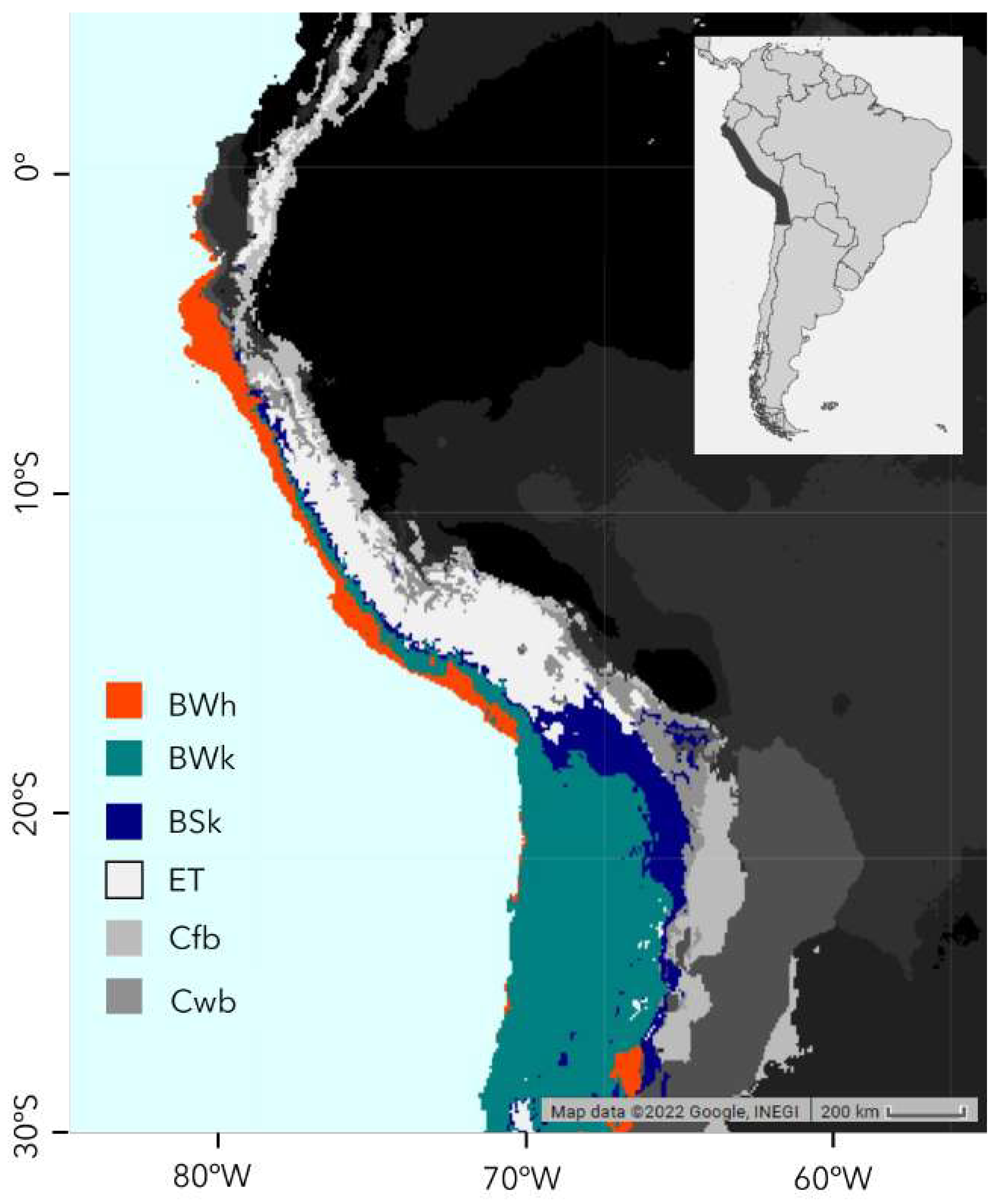
Figure 2.
MODIS imagery analysis workflow. Boxes with shadows represent inputs from other data sets. Boxes with rounded corners represent final results. Boxes with dotted outlines represent steps where data is discarded or excluded from analysis. Bolded outlines are repeated processes.
Figure 2.
MODIS imagery analysis workflow. Boxes with shadows represent inputs from other data sets. Boxes with rounded corners represent final results. Boxes with dotted outlines represent steps where data is discarded or excluded from analysis. Bolded outlines are repeated processes.
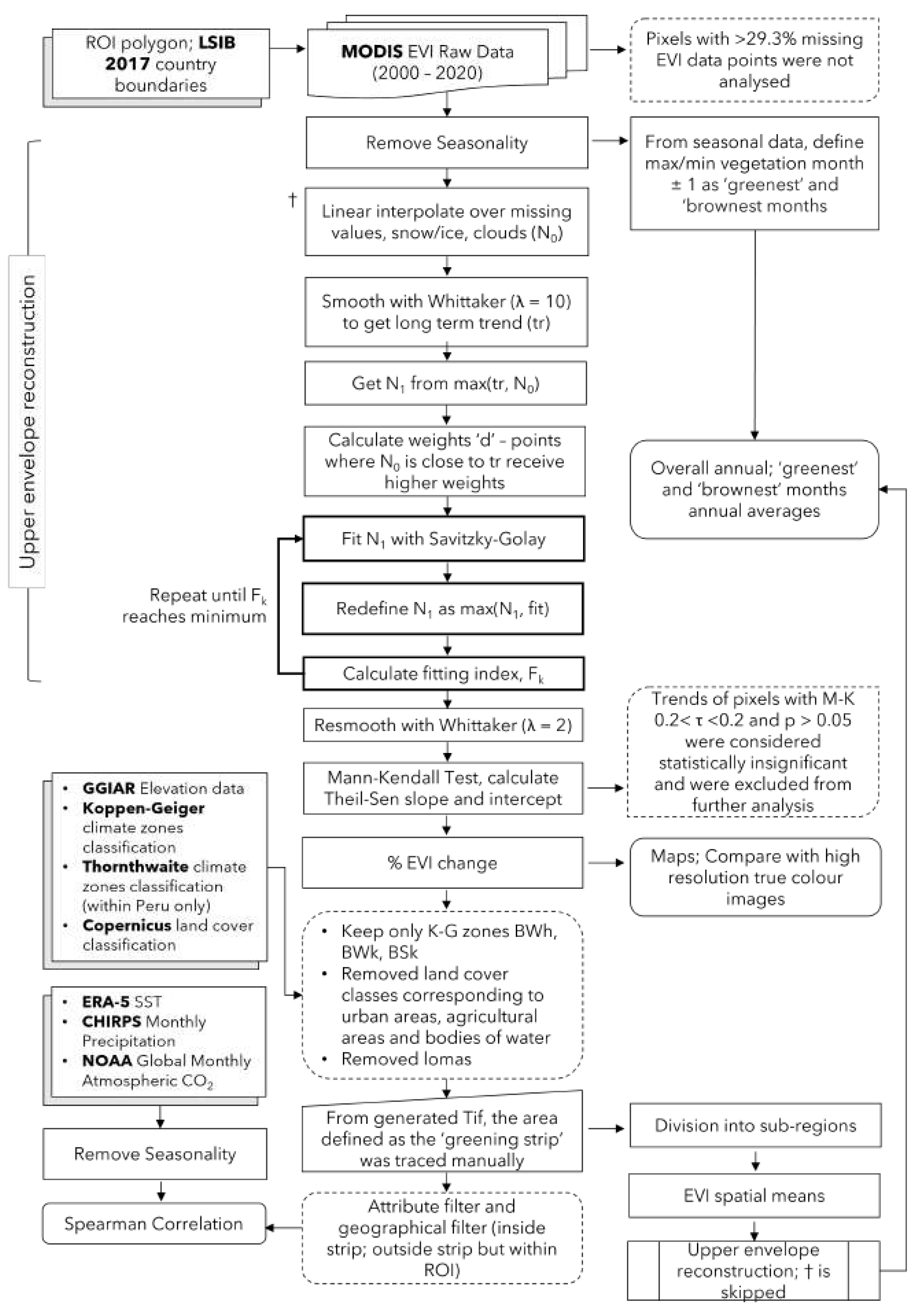
Figure 3.
The area defined as the greening strip extends from approximately 7.5S to 22.5S, located on the western flank of the Andes. The colour range includes pixels with EVI change between -10% and 60%, where change below -10% and above 60% were clipped. The inset shows statistically significant pixels only, with an EVI change of at least ±15%. Rectangular outlines in the inset show locations for higher resolution images that follow in Figure 4, Figure 5, Figure 6, Figure 7 and Figure 8.
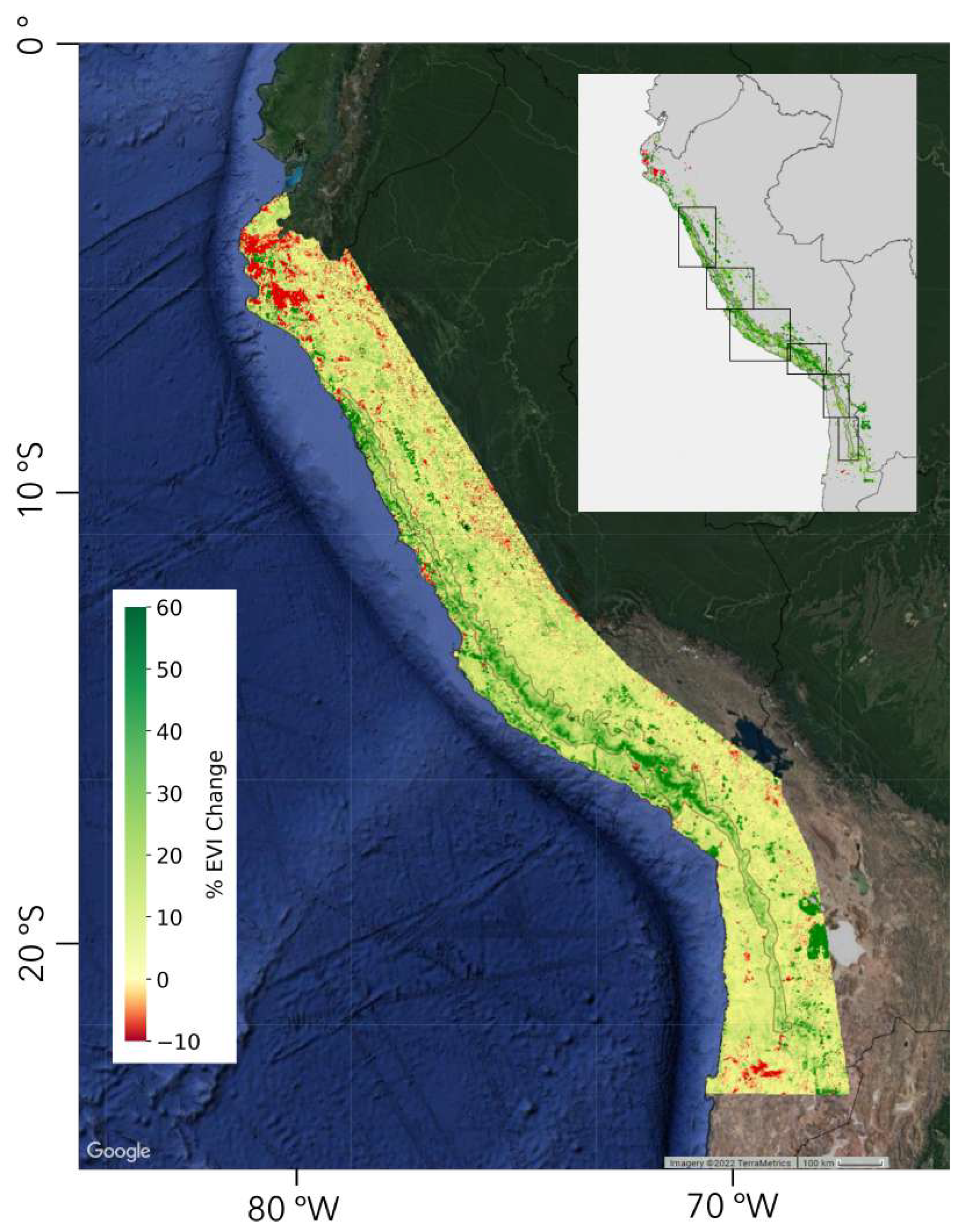
Figure 4.
There is a greening gap from approximately 9.6S to 10.2S. Dotted outlines denote urban areas and dashed outlines denote mines and quarries. Unmarked large dark green areas along the coast and smaller red areas are linked to agriculture; these were excluded from the ’greening’ strip. The dark green area towards the right hand side marks the outline of glaciers.
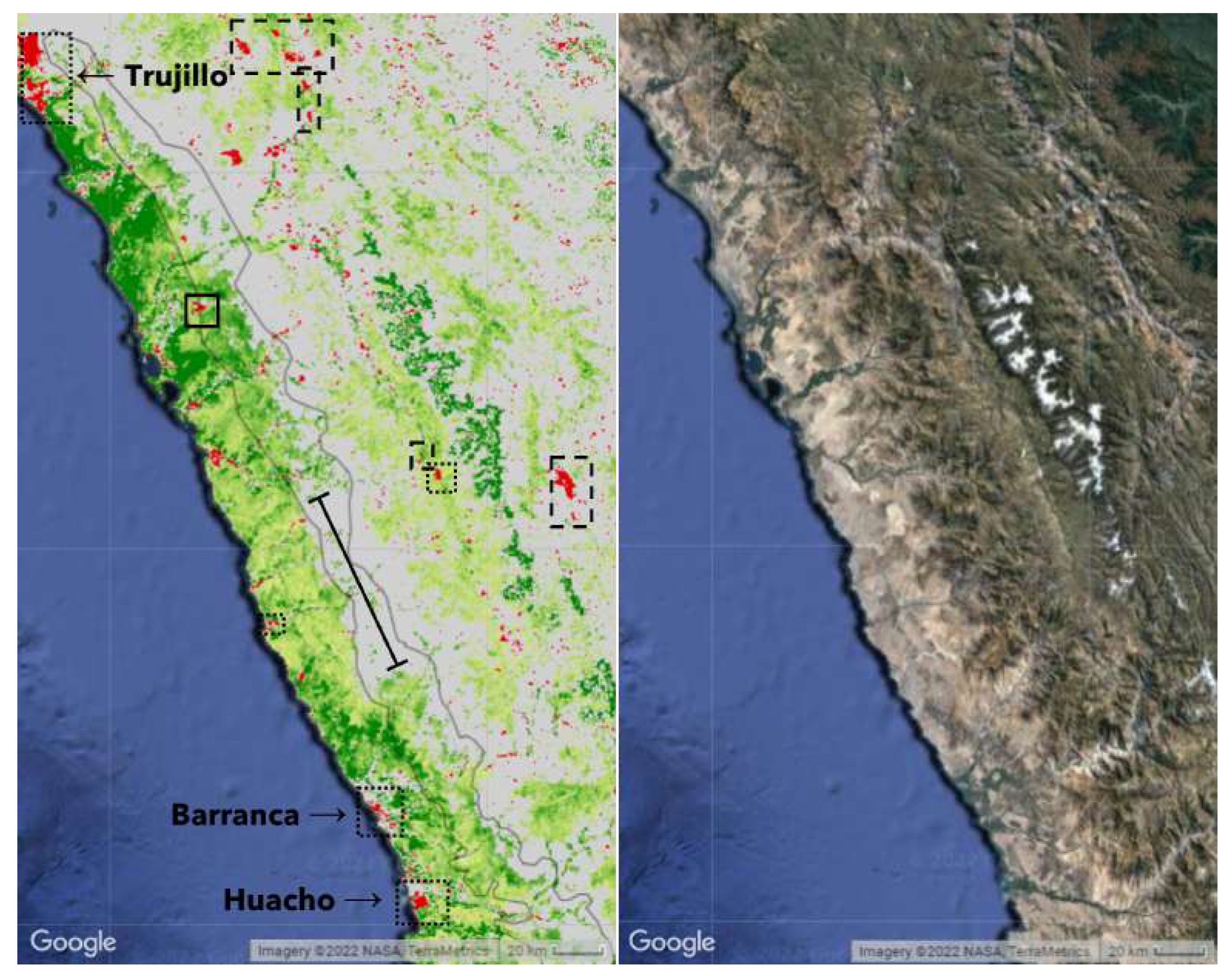
Figure 5.
Greening increases in intensity southwards from Lima. Dotted outlines denote urban areas and dashed outlines denote mining activity. The solid tipped arrow represents separation between the strip and other, less intense, natural greening closer to the coast. The smaller coastal greening is located in a different geographical region and was not included in what we define as the greening strip. Red patches seen on the coast are urban areas. Red lines crossing the strip are roads and green lines are rivers. Solid outlines denote agricultural and farming areas.
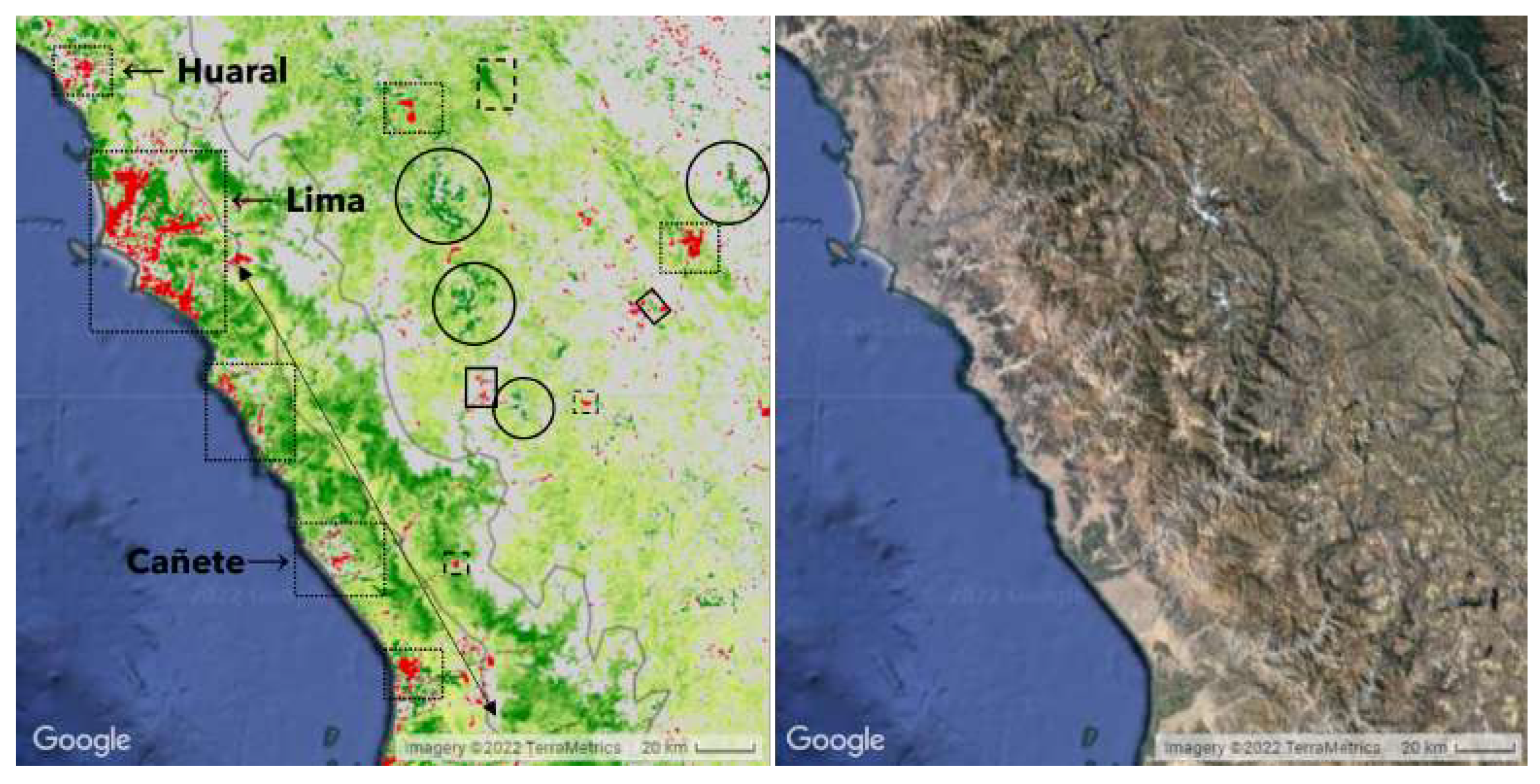
Figure 6.
Dotted outlines denote urban areas and dashed outlines denote mines and quarries. The discontinuous areas of coastal greening were not included in the greening strip as they are located beneath the Pacific slope, sensu strictu. Agricultural development along rivers, highlighted using a solid box, was also excluded from our statistical analysis, since any change in vegetation would be directly controlled by human activity. Similarly, red stripes perpendicular to the coast going into the strip are either roads or abandoned or less productive fields along rivers and were excluded from our analysis. Solid circles outline glaciers.
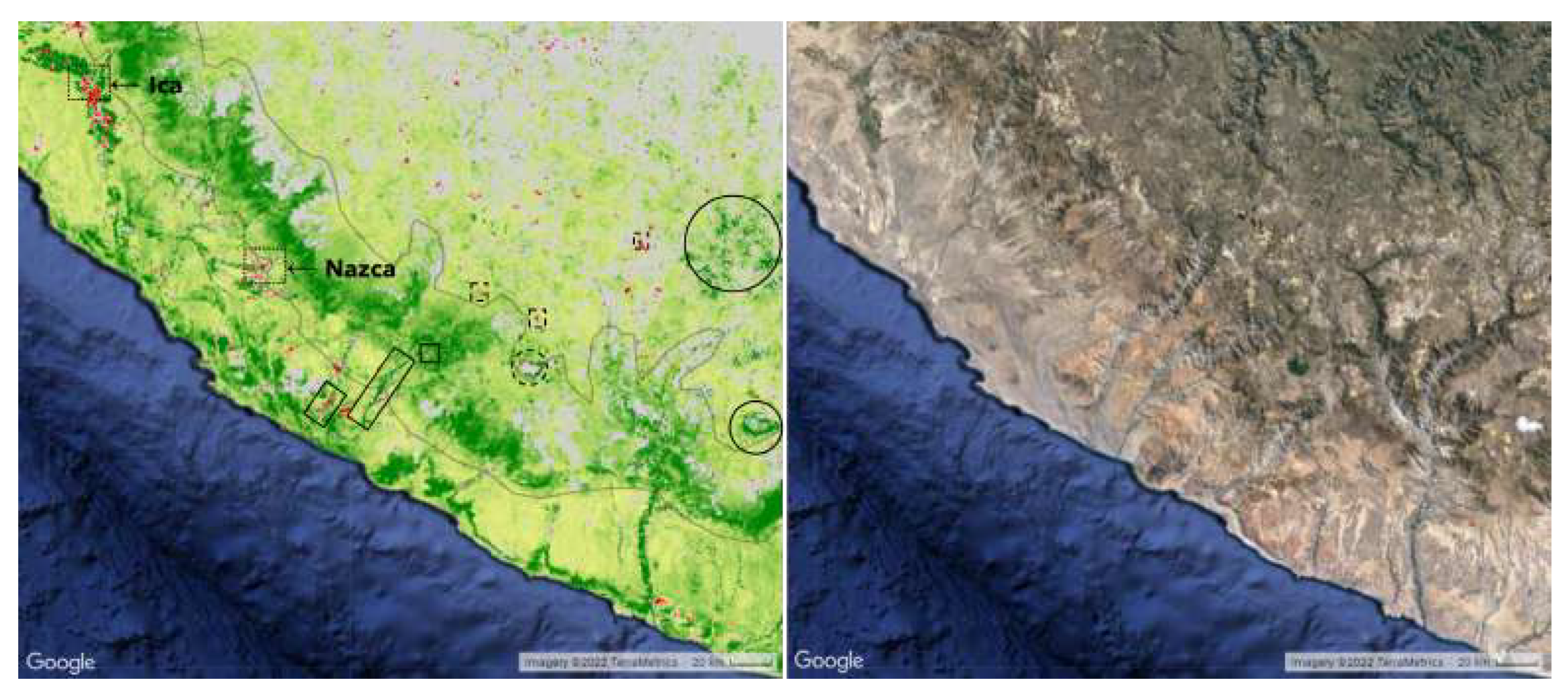
Figure 7.
Dotted outlines denote urban areas and dashed outlines denote mines and quarries. Large marked red/green patches are cities and agricultural areas – most of these pixels have been excluded from our analysis. Red or green lines extending from the coast up into the greening strip are rivers and roads. Pixels within the greening strip exhibit the most intense relative increase in the area located between Arequipa and Moquegua. Solid circles outline glaciers.
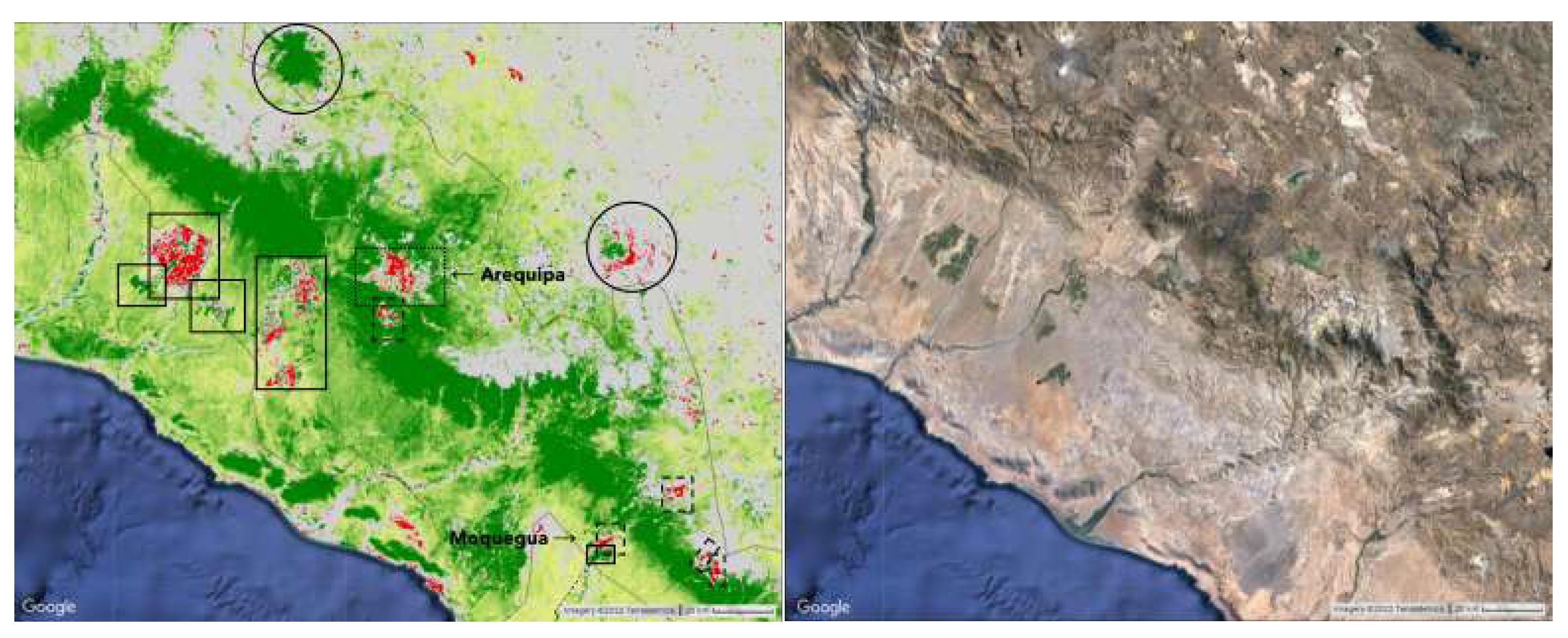
Figure 8.
Dotted outlines denote urban areas and dashed outlines denote mines and quarries. Left: The greening of coastal vegetation, as seen in Figure 6 and Figure 7, stops. Red or green lines extending from the coast up into the greening strip are rivers and roads. Right: Between 19.9S and 20.2S, another gap in the greening strip can be found. South of this area, the greening of vegetation becomes less intense and the strip is no longer visible.Solid circles outline glaciers.
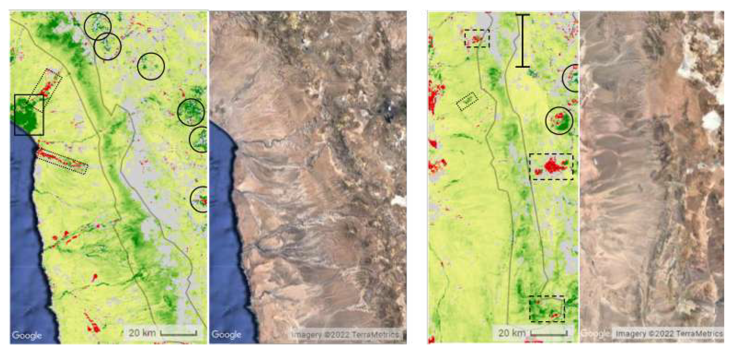
Figure 9.
Visualisation of relative EVI change as a function of both latitude and altitude. Latitude cross-sections were taken from Northern Peru to Northern Chile.
Figure 9.
Visualisation of relative EVI change as a function of both latitude and altitude. Latitude cross-sections were taken from Northern Peru to Northern Chile.
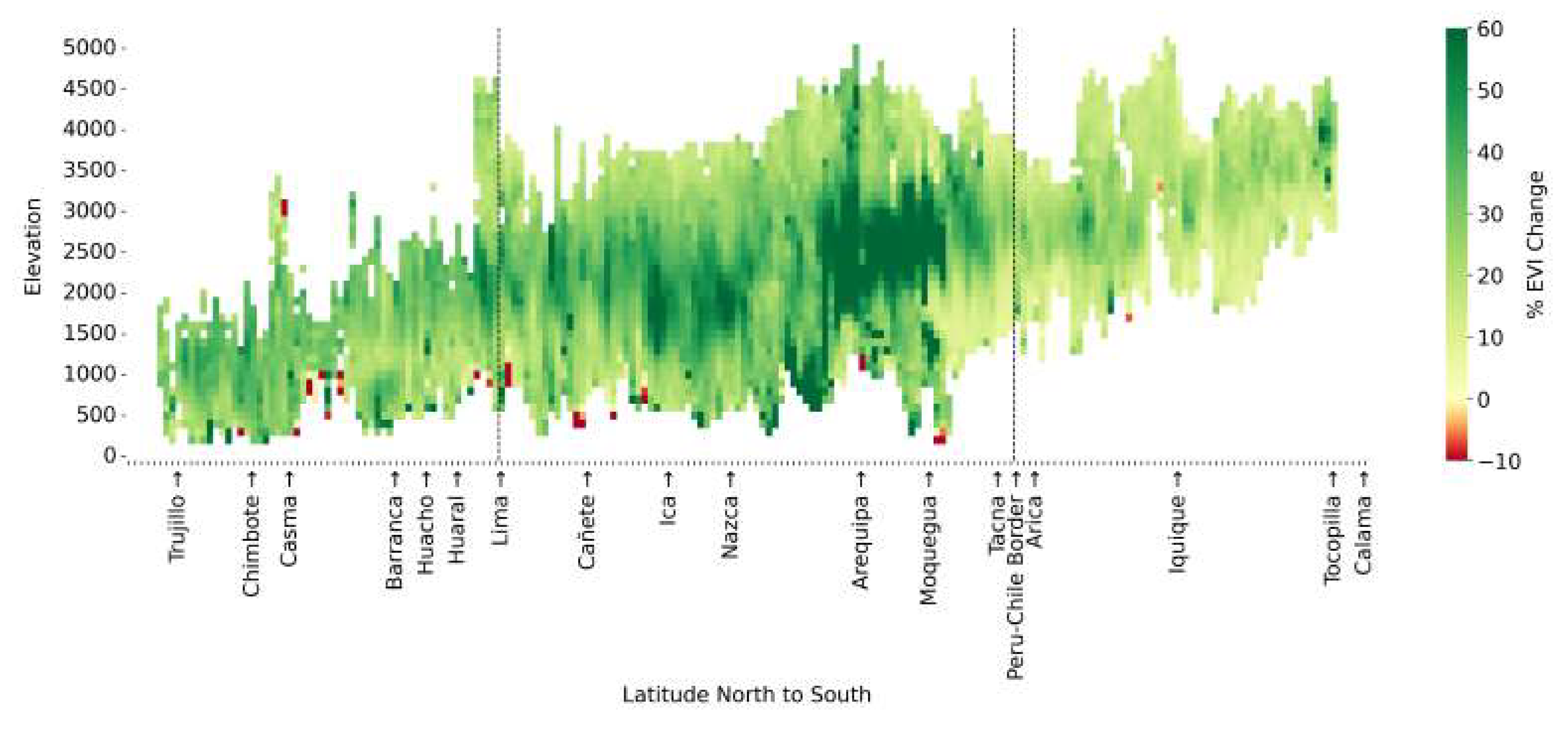
Figure 10.
Binned distributions of statistically significant EVI changes.
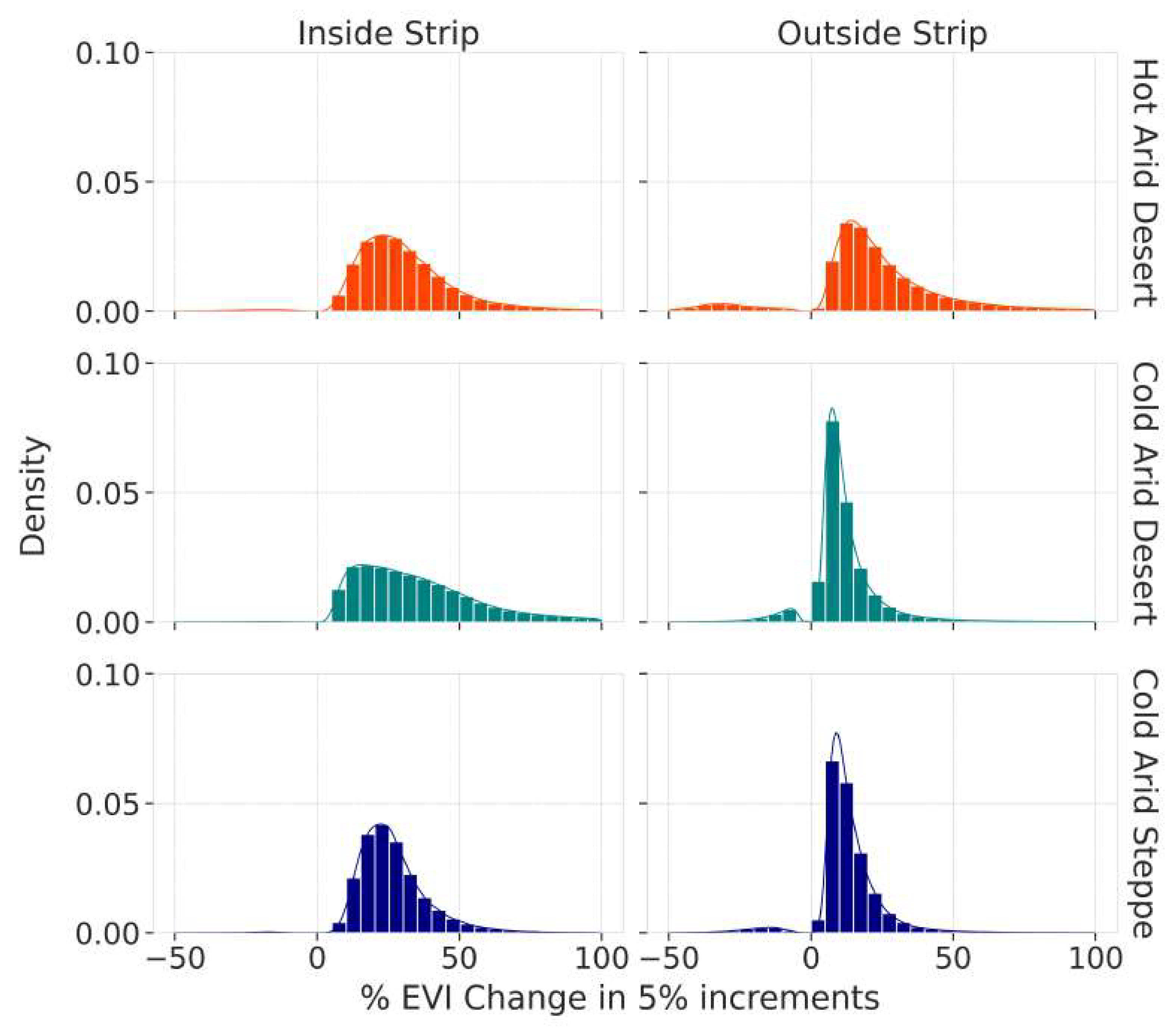
Figure 11.
Monthly time series of spatially averaged EVI across the greening strip (solid dark green line) compared to monthly precipitation, sea surface temperature (SST) and atmospheric . Orange and blue shaded areas represent the duration of El Niño and La Niña events, respectively, where darker colours denote more intense events [74]
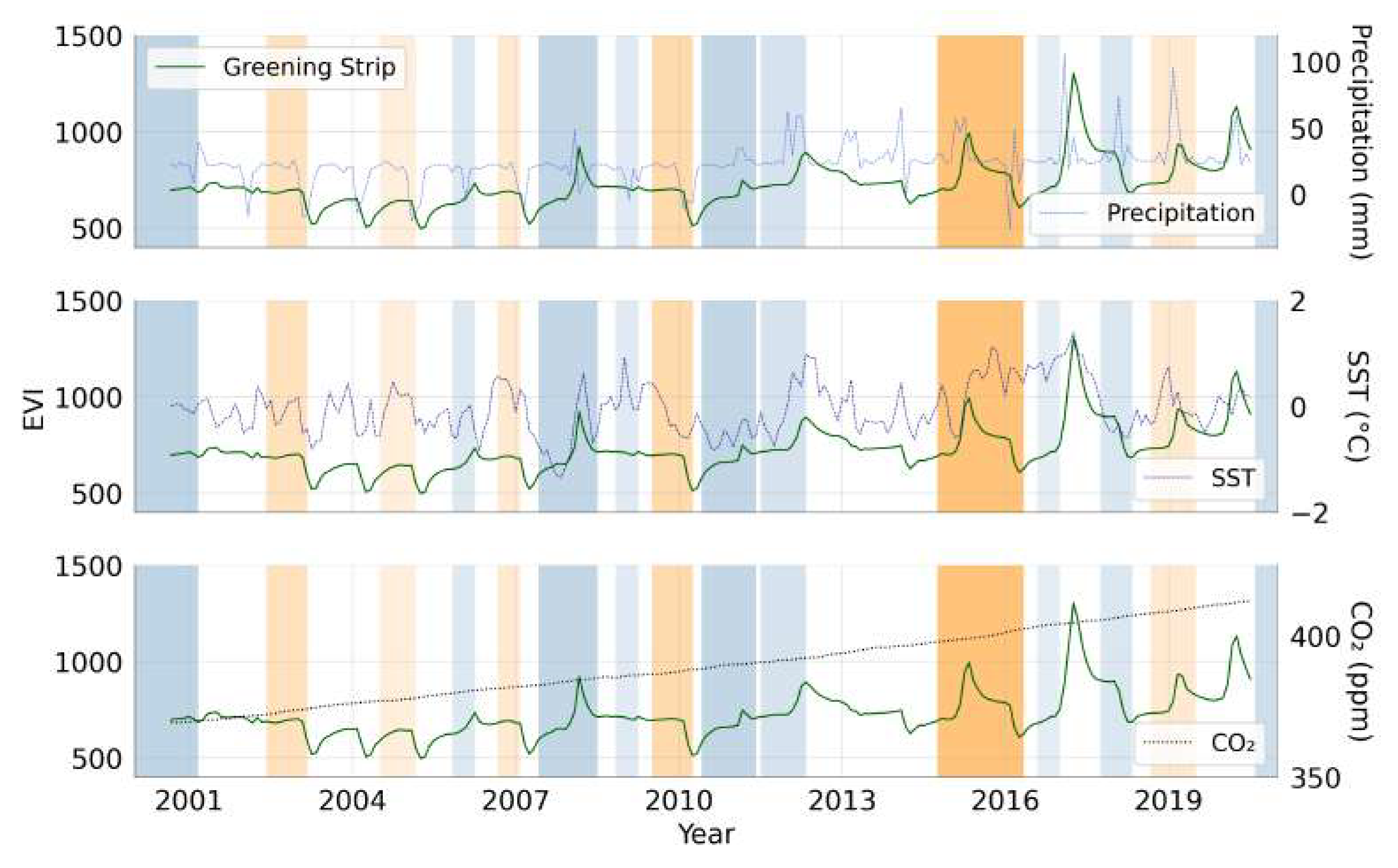

Table 1.
Study area composition, as defined by Köppen-Geiger zones [4] totalling over 99% of the area. The climate zone code relates to the legend in Figure 1. We limited our study to the Pacific slope of the Andes, thus, we manually excluded the climate zones on the eastern side of the continental divide, coloured in light gray.
| Climate Zone | Code | Area Coverage |
|---|---|---|
| Arid, Desert, Cold | BWk | 30.0% |
| Polar, Tundra | ET | 29.2% |
| Arid, Desert, Hot | BWh | 16.7% |
| Arid, Steppe, Cold | BSk | 7.9% |
| Temperate, no dry season, warm summer | Cfb | 6.1% |
| Temperate, dry winter, warm summer | Cwb | 5.2% |
| Tropical, savannah | Aw | 2.0% |
| Arid, steppe, hot | BSh | 1.3% |
| Tropical, rainforest | Af | 0.9% |
Table 2.
Correlations between spatially averaged EVI time series within Köppen-Geiger climate zones. Cells highlighted in light grey represent correlations between the same climate zone inside vs. outside the greening strip; dark grey represents correlations between different zones inside the greening strip.
| BWk | BSk | GS | GS_BWh | GS_BWk | GS_BSk | |
|---|---|---|---|---|---|---|
| BWh | 0.85 | 0.82 | 0.72 | 0.92 | 0.71 | 0.59 |
| BWk | 0.79 | 0.63 | 0.78 | 0.60 | 0.54 | |
| BSk | 0.69 | 0.79 | 0.67 | 0.64 | ||
| GS | 0.75 | 0.997 | 0.92 | |||
| GS_BWh | 0.72 | 0.60 | ||||
| GS_BWk | 0.91 |
Table 3.
Cross-correlation of the EVI time series in the greening strip and each Köppen-Geiger climate zone with precipitation, sea surface temperature and global CO concentrations.
Table 3.
Cross-correlation of the EVI time series in the greening strip and each Köppen-Geiger climate zone with precipitation, sea surface temperature and global CO concentrations.
| Region | Precipitation | SST | Global |
|---|---|---|---|
| BWh | 0.65 | 0.26 | 0.93 |
| BWk | 0.36 | 0.18 | 0.85 |
| BSk | 0.28 | 0.19 | 0.77 |
| GS | 0.53 | 0.38 | 0.60 |
| GS_BWh | 0.57 | 0.27 | 0.83 |
| GS_BWk | 0.52 | 0.39 | 0.58 |
| GS_BSk | 0.45 | 0.37 | 0.46 |
Disclaimer/Publisher’s Note: The statements, opinions and data contained in all publications are solely those of the individual author(s) and contributor(s) and not of MDPI and/or the editor(s). MDPI and/or the editor(s) disclaim responsibility for any injury to people or property resulting from any ideas, methods, instructions or products referred to in the content. |
© 2023 by the authors. Licensee MDPI, Basel, Switzerland. This article is an open access article distributed under the terms and conditions of the Creative Commons Attribution (CC BY) license (http://creativecommons.org/licenses/by/4.0/).
Copyright: This open access article is published under a Creative Commons CC BY 4.0 license, which permit the free download, distribution, and reuse, provided that the author and preprint are cited in any reuse.


