Submitted:
28 April 2023
Posted:
28 April 2023
You are already at the latest version
Abstract
In this work, we consider two SIR patterns with demography: the classical pattern and a modified pattern with a linear transmission coefficient of the infection. By reformulating of each first order differential systems as a system with two second-order differential equations, we investigate the nonlinear dynamics of the system from the Jacobi stability point of view by using the KCC geometric theory. We will study the intrinsic geometric properties of the systems by determining the geometric associated objects: the zero-connection curvature tensor, the nonlinear connection, the Berwald connection, and the five KCC invariants: the first invariant - the external force εi, the second invariant - the deviation curvature tensor Pji, the third invariant - the torsion tensor Pjki, the fourth invariant - the Riemann-Christoffel curvature tensor Pjkli, and the fifth invariant - the Douglas tensor Djkli. In order to obtain necessary and sufficient conditions for the Jacobi stability near the equilibrium points, the deviation curvature tensor will be determined at each equilibrium points. Furthermore, we will compare the Jacobi stability with the classical linear stability, inclusive by diagrams related to the values of parameters of the system.
Keywords:
SIR pattern
; KCC theory
; the deviation curvature tensor
; Jacobi stability
1. Introduction
Mathematical patterns that do not explicitly include births and deaths occurring in the population are called epidemic patterns without demography. They are useful for epidemic modeling on a short time scale, particularly for modeling some epidemic like influenza. Omitting population change requires that the disease develop on a much shorter time scale than the period in which significant change in the population size can occur (such as births and deaths). This is valid for fast diseases like the childhood diseases and influenza. On the other hand, there are slow diseases, such as HIV, tuberculosis, and hepatitis C, that develop for a long period of time even on an individual level. In this case, the total population does not remain constant for long periods of time, and the demography of the population cannot be ignored [1,2,3].
The main goal of the present paper is to study the Jacobi stability for two SIR models with demography: the classical SIR model and a modified SIR model with a variable transmission coefficient of the infection (linear with respect to the number I of the infected individuals). The classical stability (linear or Lyapunov stability) of different kinds of SIR (susceptible, infected and removed individuals) epidemic models without or with demography was widely completely studied in last decades [1,2,3,4,5,6]. In this work, we will study another type of stability for these systems, namely the Jacobi stability. Classical approaches of this models can be found in [1,2,3,4]. Generally, the study of mathematical deterministic models for the spread of diseases, or for the interaction between prey-predator type populations is performed only for positive values of the variables, where they has an ecological, biological or epidemiological meaning [4,5,6,7,8,9].
The Jacobi stability is a natural extension of the geometric stability of the geodesic flow, from a manifold with a Riemann or Finsler metric to a manifold with no metric [10,11,12,13,14,15]. Practically, the Jacobi stability indicates the robustness of a dynamical system defined by a system of second-order differential equations (or SODE), where this robustness measures the lack of sensitivity and adaptation to both the modifications of the internal parameters of the system and the change in the external environment. By using the Kosambi–Cartan–Chern (KCC) theory, the local behavior of dynamical systems from the point of view of the Jacobi stability has recently been studied by several authors in [11,12,16,17,18,19,20,21,22,23,24,25,26]. Hence, the local dynamics of the system is investigated by using the geometric objects that correspond to the system of the second-order differential equations (SODE), which is the system obtained from the given first-order differential system [27,28,29].
The KCC theory deals with the study of the deviation of neighboring trajectories, which allows us to to estimate the perturbation permitted around the equilibrium points of the second-order differential system. Initially, this approach was linked with the study of the variation equations (or Jacobi field equations) associated with the geometry on the differentiable manifold. More exactly, P. L. Antonelli, R. Ingarden, and M. Matsumoto started the study of the Jacobi stability for the geodesics corresponding to a Riemannian or Finslerian metric by deviating the geodesics and using the KCC-covariant derivative for the differential system in variations [10,11,12]. As a result, the second KCC-invariant appeared, also called the deviation curvature tensor, which is essential for the establishment of the Jacobi stability for geodesics and generally for the trajectories associated with a system of second-order differential equations. In differential geometry, a system of second-order differential equations (SODE) is called semi-spray. Using a semi-spray, we can define a nonlinear connection on the manifold, and conversely, using a nonlinear connection, we can define a semi-spray. Consequently, any semi-spray (or SODE) can define a geometry on the manifold by the associated geometric objects, and conversely [13,30,31,32]. Of course, these geometric objects are tensors that can check the properties of symmetry or not, depending on the particularity of the system of second-order differential equations (SODE).
The KCC theory originated from the works of D. D. Kosambi [27], E. Cartan [28], and S. S. Chern [29]; hence, the abbreviation KCC (Kosambi–Cartan–Chern). This geometric theory can be successfully applied in many research fields, from in engineering, physics, chemistry, and biology [16,19,21,23,24,33]. In addition, new approaches and results from the KCC theory in gravitation and cosmology were made in [34,35]. Moreover, in [18], a comprehensive analysis of the Jacobi stability and its relations with the Lyapunov stability for dynamical systems was made by C.G. Boehmer, T. Harko, and S.V. Sabau, who modeled the phenomena based on gravitation and astrophysics. Recently, in [36], a very interesting and complete study of the Jacobi stability for prey–predator models of Holling’s type II and III was performed.
In the second section, there will be a short, but comprehensive presentation of the classical SIR epidemic model with demography, and we will point out the main results on the local and global stability of this system. Next, in the third section, a reformulation of the classical SIR epidemic model with demography (3) as a system of second-order differential equations will be obtained, and the five geometrical invariants for this system will be computed. The obtained results for the Jacobi stability of this system near the equilibrium points will be presented in the fourth section. More precisely, we will find the necessary and sufficient conditions that would allow us to obtain the Jacobi stability of the system near the equilibrium points. Consequently, for these parameter values, it is not possible to have a chaotic behavior for the classical SIR epidemic model with demography. Furthermore, at the end of the fourth section, we will obtain the deviation equations near every equilibrium point as well as the curvature of the deviation vector, and then we perform a comparative analysis of the Jacobi stability and the Lyapunov stability in order to compare these two approaches. Using the same approach, in the fifth section we will obtain similar results for a classical SIR epidemic model with demography and vaccination.
Further, a modified SIR epidemic model with demography with a linear transmission coefficient of infection was presented in the sixth section [1]. After a second order reformulation of this modified SIR model in the seventh section, the Jacobi stability analysis of this system was done in the section eight. Conclusions and possible future research was presented in the last section.
At the end, in the appendix A was presented a comprehensive review of the basic notions and main tools of the KCC theory that are necessary for analyzing the Jacobi stability of dynamical systems. More exactly, we will present the five invariants of the KCC theory and the definition of the Jacobi stability. As usual in differential geometry, the sum over the crossed repeated indices is understood.
2. A Classical SIR Epidemic Pattern with Demography
A classical SIR epidemic model for the spread of the diseases suppose that the whole population at a time t is split in three categories: is the number of individuals which are susceptible at the moment t, is the number of the infected individuals at t and represent the number of removed individuals at the time t, where by a removed individual we understand individuals either recovered from the illness or dead after the infection [1,2,3,4,5,6]. A SIR model without demography means that the total number of individuals is constant, i.e. no born, no immigration, no dead and no emigration. But, practically this reality it is not possible and then it was considered different SIR models with demography, for which is not constant. To incorporate the demographics into a classical SIR epidemic model, we assume that all individuals are born susceptible [1]. Individuals from each category die at a per capita death rate , so the total death rate in the susceptible category is , while in the infectious category, it is , and in the removed category, it is . If we denote by the recovery rate, then the rate of the recoveries in the infected people is . Also, as for the SIR model without demography, if we will denote by the transmission coefficient of the infection, then we can consider the following classical SIR model with demography:
where is the total birth rate (measured in number of people born per unit of time) and , , denote the derivatives with respect to time t, or the rates of changes of these quantities in a short unity of time.
Let us remark that the third equation of the system (1) was added in order to obtain the next differential equation for the total population :
with the unique solution . Therefore, the population size is not constant, but it is asymptotically constant, since when .
Obviously, we can observe that the first two equations in (1) are independent of the third, and then we can consider the two-dimensional autonomous system of first order differential equations:
where .
Compared to - the transmission coefficient of the infection, which has the unit [number of people × time], the parameters - the recovery rate and - the dead rate, have the units [unit of time]. So, it is better to consider and then is a dimensionless quantity. If we denote and , then we have and , by using the chain rule. After resizing the variables and with the total limiting population size , we will obtain the new variables and , which are also dimensionless quantities.
Therefore, we can say that the system (2) was transformed into a system with dimensionless form (3), which is equivalent to the original one, since the solutions of both systems have the same long-term behavior. Moreover, the number of parameters was reduced from four to two. The notation is not choose randomly, because this dimensionless quantity is indeed the reproduction number or the basic reproduction number for this mathematical epidemiological pattern [1,5,6].
Because it is impossible to solve the first order differential system associated to this SIR pattern with demography by analytical methods, it remains only to find information about the behavior of the solutions. Especially, because we want to know what will happen to the disease in the long run: will it go out, or will it establish itself in the population and become endemic? So, the long-term behavior of the solutions is very important from an epidemiological perspective [1,2,3].
It is clear that the model has relevance when , , and then the solutions of the system (3) lie in the first quadrant . Moreover, the lines and are invariant manifolds with respect to the flow of the system, that means any orbit starting from a point which belongs to remains in . So, the orbits cannot cross any of these two invariant lines and then the study of the system where it has a epidemiological relevance is well-defined, in the sense that, an orbit starting from a zone with epidemiological relevance does not enter in a zone with epidemiological irrelevance and conversely.
However, it is very important to study the local dynamics of the system with the classical tools of dynamical systems and, also, by geometrical tools of Kosambi-Cartan-Chern (KCC) theory. First of all, we must determine the equilibrium points of the epidemic given by dynamical system (3), by solving the system
and so we get two equilibrium points , so-called the disease-free equilibrium, and , so-called the endemic equilibrium.
Let us remark that the endemic equilibrium exists if and only if the basic reproduction number . Else, if , then coincides with , or, if , then is a virtual equilibrium point, i.e. don’t belongs to and then is irrelevant.
According to Hartman-Grobman Theorem, it is known that the local stability of hyperbolic equilibrium points is determined by the eigenvalues of the Jacobi matrix computed at each equilibrium point. Because the Jacobi matrix of the system (3) at the point is
it results that:
- For the disease-free equilibrium , the Jacobi matrix is with eigenvalues , . Then is unstable (saddle point) if and only if , and is locally asymptotically stable (stable node) if and only if . If , then is a non hyperbolic equilibrium point and we cannot apply Hartman-Grobman Theorem for the local behavior study.
-
For the endemic equilibrium , the Jacobianwith characteristic polynomial and eigenvalues. Since , we have that and , that means that, if exists, the endemic equilibrium is always locally asymptotically stable (stable node or stable focus). More precisely, is a stable node if and only if , and is a stable focus if and only if .
In conclusion, the basic reproduction number of the disease modelled by (3) has the next threshold role [1,5,6]:
- If , then there exists only the disease-free equilibrium point, which is an attractive equilibrium (stable node), i.e. any trajectory of the dynamical system (3) starting near to converges at this equilibrium when time tends to infinity, and the disease disappears from the population.
- If , then there exists two equilibrium points: the disease-free equilibrium and the endemic equilibrium. The disease-free equilibrium is not attractive (unstable, a saddle point), in the sense that there exists trajectories of the system (3) that start very close to , but it tend to go away. Instead, the endemic equilibrium is attractive (stable node or stable focus), that means any orbit of the system (3) starting near to converge to as time goes to infinity. So, in this case, the disease remains endemic in the population.
Related to the global stability, an equilibrium point is called globally stable if it is stable for almost all initial conditions, not just those that are close to it. For this classical SIR system are known the following results [1,5] (see also the Dulac–Bendixson Theorem):
Theorem 2.1
a) For , the disease-free equilibrium is globally stable.
b) For , the system (3) has no periodic orbits.
c) For , the endemic equilibrium is globally stable whenever .
In conclusion, we collect the obtained results for the local stability in the next Table 1:
In the next sections, we will focus only on the study of the Jacobi stability in order to clarify the behavior of the SIR system and to point out the geometric objects associated to this system of ordinary differential equations.
3. SODE Formulation of the Classical SIR Pattern with Demography
We consider the classical SIR model with demography (3). For the sake of simplicity we will denote the derivative with respect to time with "dot" over the variable and we prefer to denote t instead of . Then the system (3) becomes
where and .
By taking the derivative with respect to time t in both equations of this system, we obtain the following second order differential equations:
In order to use the rule of the crossed repeated indices from differential geometry formalism, we change the notations of variables as follows:
Then this system of second-order differential equations (SODE) becomes:
or, equivalently,
where , .
This system can be written similarly to a SODE (semi-spray) from the KCC theory:
where
The zero-connection curvature is given by the next coefficients:
The nonlinear connection N has the following coefficients:
Consequently, all coefficients of the Berwald connection are null.
The first invariant of the KCC theory has the following components:
Let us remark that for , which means that for , or equivalently, the functions are 1-homogeneous with respect to .
Next, by using (A10), we obtain the components of the second invariant of the KCC theory, which means that the deviation curvature tensor of the classical SIR model with demography (4) is as follows:
Then, the trace and the determinant of the following deviation curvature matrix:
are tr and .
Following Theorem A2, we have:
Theorem 3.1
All the roots of the characteristic polynomial of P are negative or have negative real parts (i.e., Jacobi stability) if and only if
Taking into account that , , , we obtained the third, fourth, and fifth invariants of the classical SIR model with demography (4) as follows:
Theorem 3.2
The third KCC invariant , called the torsion tensor, has all eight components null, i.e.,
The fourth KCC invariant , called the Riemann–Christoffel curvature tensor, has all sixteen components null, i.e.,
The fifth KCC invariant , called the Douglas tensor, has all sixteen components null, which means that
4. Jacobi Stability Analysis of the Classical SIR System with Demography
In this section, we will determine the first two invariants at the equilibrium points of the SIR model with demography (4), and we will analyze the Jacobi stability of the system near each equilibrium point.
Furthermore, for equilibrium points and of the initial SIR model with demography (3), we have the corresponding equilibrium points and for SODE (6).
For , the first invariant of the KCC theory has the components , and the matrix with the components of the second KCC invariant is as follows:
Since and , by using Theorem 3.1, we obtain the following result:
Theorem 4.1
The disease-free equilibrium point is always Jacobi unstable.
For the first invariant of the KCC theory has the components , , and the matrix with the components of the second KCC invariant is as follows:
Since and , by using Theorem 3.1, we obtain the following result:
Theorem 4.2
The endemic equilibrium point is Jacobi stable if and only if .
Remark 4.3.
Whenever exists and is Jacobi-stable, a chaotic behavior of the SIR system in a small enough neighborhood of this point is not possible.
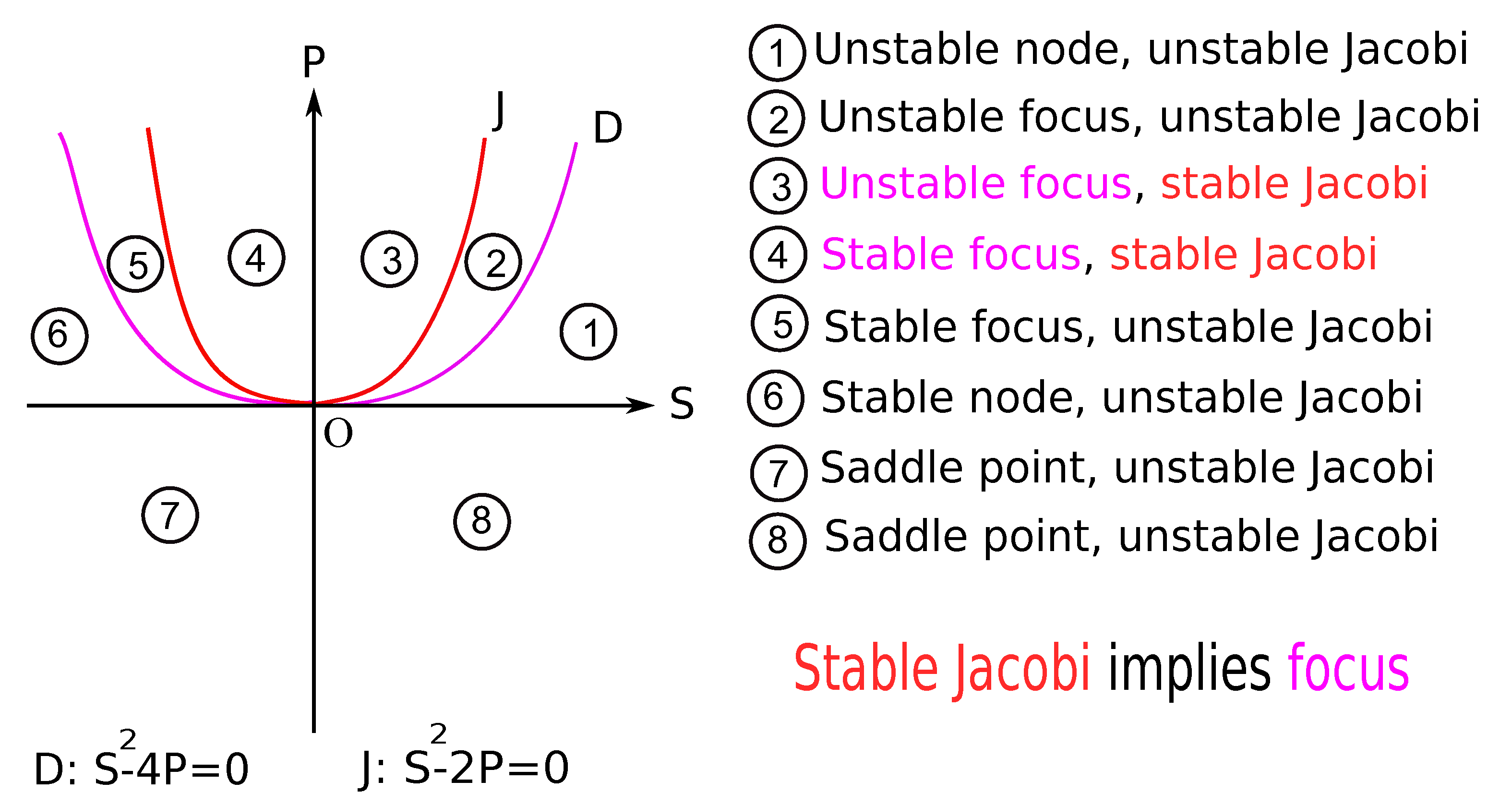
In order to more clearly represent the relationship between linear (or Lyapunov) stability and Jacobi stability for this SIR system, we will consider the following diagram with respect to the parameters and of the system (see Figure 1):
Taking into account that , and according with Theorem 4.2, we obtain the following result:
Theorem 4.4
If the endemic equilibrium point exists, then it is Jacobi-stable if and only if the reproduction number satisfies the conditions:
Proof.
By using the Jacobi stability condition from Theorem 4.2 and the study of the sign of the second order function in , , with the discriminant equal with , the theorem is proved. □
According to the expression of the characteristic polynomial at the endemic equilibrium point , we get the next result about the local linear stability of the endemic equilibrium.
Theorem 4.5
If exists, the endemic equilibrium , is a stable focus if and only if the reproduction number satisfies the conditions:
Otherwise, the endemic equilibrium is a stable node.
Proof.
Because the discriminant associated to the characteristic polynomial at is equal with , is necessary to study the sign of the second order function in , . □
Let us remark that apart from the reproduction number , the parameter is the most important parameter of this epidemic model. Only if (i.e. ), the endemic equilibrium (if exists) can be stable from the Jacobi point of view. Therefore, recovery rate from illness plays an unexpectedly crucial role both for Lyapunov stability and for Jacobi stability of this classical SIR system.
In order to obtain characterizations of the local stability of the endemic equilibrium point related to the parameter - the transmission coefficient of the infection, the next results are obtained:
Theorem 4.6
If the endemic equilibrium point exists, then it is Jacobi-stable if and only if the transmission coefficient β satisfies the conditions:
where is the limit size of the entire population.
Proof.
By replacing both dimensionless parameters and with the four parameters of the initial system (1), and using the Jacobi stability condition from Theorem 4.2, the theorem is proved by following the sign of the second order function in , , with the discriminant equal with . □
Theorem 4.7
If exists, the endemic equilibrium , is a stable focus if and only if the transmission coefficient β satisfies the conditions:
where is the limit size of the entire population.
Otherwise, the endemic equilibrium is a stable node.
Proof.
Because the discriminant associated to the characteristic polynomial at is equal with , is necessary to study the sign of the second order function in , . □
If the mortality rate is known at a value , in order to obtain threshold values of the parameter , the recovery rate, it is enough to replace with in Theorem 4.2 and it results:
Theorem 4.8
a) If the endemic equilibrium point exists, then it is Jacobi-stable if and only if the recovery rate α fulfills the condition:
b) If exists, the endemic equilibrium , is a stable focus if and only if the recovery rate α fulfills the condition:
Otherwise, the endemic equilibrium is a stable node.
Let us remark that , i.e. because the Jacobi stability of an equilibrium point implies that this equilibrium is a focus.
Conversely, if we fixed the value of the recovery rate at the value , then we obtain the following threshold values for the mortality rate :
Theorem 4.9
a) If the endemic equilibrium point exists, then it is Jacobi-stable if and only if the mortality rate μ fulfills the condition:
b) If exists, the endemic equilibrium , is a stable focus if and only if the mortality rate μ fulfills the condition:
Otherwise, the endemic equilibrium is a stable node.
Of course, because .
4.1. Dynamics of the Deviation Vector for the Classical SIR System with Demography
The behavior of the deviation vector , , giving the trajectory behavior of the dynamical system near an equilibrium point is described by the deviation equations (or Jacobi equations) (A8), or in a covariant form such as equations (A9).
For this classical SIR system with demography, the deviation equations become:
The length of the deviation vector is given by
Next, we will write the deviation equations near to each equilibrium point for the classical SIR system with demography. Then, the dynamics of the deviation vector near to the disease-free equilibrium point is described by the following SODE:
The dynamics of the deviation vector near to the endemic equilibrium point
is described by the deviation equations:
5. A Simple SIR Epidemic Pattern with Demography and Vaccination
In this section we propose a classical and simple SIR model with vaccination as in [37]. Also, a very interesting four dimensional model with vaccination was studied recently in [38]. Next, we will reconsider the classical SIR model with demography (1) and we will assume that a part of the susceptible individuals are vaccinated with the rate of vaccination p. According to the classical SIR model this vaccination rate is measured in [unit of time]. If we will suppose that all vaccinated individuals will not be infected and more that, they can be considered to belongs to the catogory of removed individuals, then the model (1) becomes
Let us observe that the first two equations of the system (20) are independent of the third equation, because we can obtain the removed population by using and due to the fact that the total population can be obtained from the differential equation
with the unique solution .
Obviously, as for the classical model (1), the population size is not constant, but it is asymptotically constant, since when .
Taking into account all these proposals, we can consider the two-dimensional autonomous system of first order differential equations:
By applying similar techniques as in Section 2 and by changing of time and variables, , , , where , , we obtain the equivalent dimensionless form of (21):
where and are both dimensionless parameters.
Let us remark that system (22) is exactly the dimensionless system (3) obtained for the classical SIR model in Section 2. Therefore, all obtained results remain available also for this SIR epidemic model with demography and vaccination. Only interpretations can be different because the dimensionless parameters and are different. Of course, is the basic reproduction number for this model. Moreover, the number of parameters was reduced from five to two.
According to the expressions of and , it is clear that if and only if and if and only if . So, if we take account of the results presented in Figure 1, for this model the endemic equilibrium can be a stable focus only if the recovery rate is greater than the vaccination rate p and can be Jacobi stable only if the recovery rate is greater than .
6. A Modified SIR Epidemic Pattern with Demography
Taking into account that for the classical SIR model (1) we have no periodic orbits, and then Hopf bifurcations don’t occur, next we will consider a modified SIR system. More exactly, we will assume that the transmission coefficient of infection is not constant, but is a linear function of the number of infected individuals, that means is replaced by , where is a parameter [1,39]. This imply that the transmission coefficient of infection and, also, the contact rate increase with the number of infectious individuals and new infections occur much faster in comparison with the classical model [1].
Therefore, the model becomes:
Let us remark that the total population size satisfies and then we can omit the third equation for recovered individuals R. It follow that it is necessary and sufficient to study the two-dimensional autonomous system of first order differential equations:
where .
In order to obtain the dimensionless version of the system, using similar techniques as for the classical system (2), after changing the time variable t by and rescaling the variables , with the total limiting population size , we obtain the new variables , , which are dimensionless quantities. Consequently, if we denote , then the system (24) becomes:
where and are both dimensionless parameters.
Therefore, we can say that the system (24) was transformed the system into a dimensionless form (25), which is equivalent to the original one, since the solutions of both systems have the same long-term behavior. Moreover, the number of parameters was reduced from five (, , , , ) to three (, , ), all being strictly positive real numbers. Of course, represent the reproduction number for this modified SIR model and .
Further, our study for this modified SIR model has relevance when , , i.e. on the first quadrant or even on the open first quadrant .
The Jacobian matrix of the system (25) at a point is
In order to find the equilibrium points of (25), by analyzing the system,
we obtain at most three equilibrium, as follows:
For , it results , the disease-free equilibrium point, with Jacobian and eigenvalues , . Then is local asymptotically stable (stable node) if and only if , or is unstable (saddle point) if and only if . For , is a non-hyperbolic equilibrium point because .
For , we have , and then . Because , it results the roots of second order algebraic equation in y
where is the discriminant of the second order equation (26).
If we denote by , the second order function associated to the equation (26), then we have the following three cases:
Case 1. If , i.e. , then only the second root is strictly positive and we have only one endemic equilibrium point , with coordinates
Let us remark that , because , for any positive parameters and . Then, taking into account that , the Jacobian at the unique endemic equilibrium is
where the trace is and the determinant is , where , are eigenvalues of A.
Due to and , it results for any positive values of parameters. Therefore, the endemic equilibrium is local asymptotically stable (stable node or stable focus) if and only if , i.e.
Otherwise, the endemic equilibrium E is unstable (unstable node or unstable focus) if and only if , i.e.
Let us point out that, if (i.e. ), then are pure imaginary roots of the characteristic polynomial at E, with Re . In this case it is possible to have Hopf bifurcations along the curve tr , i.e
Case 2. If , i.e. , then and the roots of the equation (26) are and . Then we have that the first endemic equilibrium coincides with , and so, this equilibrium point is non hyperbolic, but the second endemic equilibrium becomes , with coordinates , .
Obviously, if and only if . The Jacobian at is , with eigenvalues , where .
Tacking into account that and , it results that is local asymptotically stable (stable node or stable focus) if and only if , i.e. . Else, is unstable (unstable node or unstable focus) if and only if , i.e. .
Let us point out that, if (i.e. ), then , i.e. are pure imaginary roots with Re . In this case it is possible to have Hopf bifurcations along the curve . More exactly, for and .
If , then . For , for any and only for .
Case 3. If , i.e. , then we have two endemic equilibrium points and , with positive coordinates given by
if and only if , that means .
More exactly, this two equilibrium points has the following coordinates:
and, respectively,
Let us remark that , because .
For the first endemic equilibrium , taking into account that , it results that the Jacobian matrix is
with and , where , are the eigenvalues of A.
Because and , it results that the sign of is given by . Since , we have and then the expression can be negative. Indeed, if we use the identity
and we observe that , for and (because for ), it result that
Therefore, the first endemic equilibrium is unstable (a saddle point) because .
For the second endemic equilibrium , taking into account that , the Jacobian matrix is
with and , where , are the eigenvalues of A.
Since and , we have that the sign of is given by . From , we have can be negative and also the expression can be negative. But, if we use the identity
we obtain that for any .
Then and the second endemic equilibrium is local asymptotically stable (stable node or stable focus) if and only of , i.e.
Otherwise, the endemic equilibrium is unstable (unstable node or unstable focus) if and only if , i.e.
Let us point out that, if (i.e. ), then are pure imaginary roots of the characteristic polynomial at , with Re . In this case it is possible to have Hopf bifurcations along the curve tr , i.e
If , i.e. , then there is an unique endemic equilibrium point , with and . The Jacobian at this is
with eigenvalues , that means that this endemic equilibrium point E is a non hyperbolic equilibrium.
If , i.e. , then there is no endemic equilibrium.
In conclusion, we collect the obtained results in the next Table 2:
Remark 6.1
Following the ideas and the same techniques as in Section 5, if we will consider the modified SIR model with demography and vaccination,
then, after changing of time and variables, we will obtain the same dimensionless system (25), where , and . All results obtained remains available also for this SIR epidemic model with demography and vaccination. Only the interpretations can be different because the dimensionless parameters ρ and are different.
7. SODE Formulation of the Modified SIR Pattern with Demography
We consider the modified SIR model with demography (25). For the sake of simplicity we will denote the derivative with respect to time with "dot" over the variable and we prefer to denote t instead of . Then the system (25) becomes
where , , .
By taking the derivative with respect to time t in both equations of this system, we obtain the following second order differential equations:
In order to use the rule of the crossed repeated indices from differential geometry formalism, we change the notations of variables as follows:
Then this system of second-order differential equations (SODEs) becomes:
or, equivalently,
where , .
This system can be written similarly to a SODE (semispray) from the KCC theory:
where
The zero-connection curvature is given by the next coefficients:
The nonlinear connection N has the coefficients :
Consequently, all coefficients of the Berwald connection are equal with zero.
The first invariant of the KCC theory has the following components:
Let us remark that for , which means that for , or equivalently, that the functions are 1-homogeneous with respect to .
Next, by using (A10), we obtain the components of the second invariant of the KCC theory, which means that the deviation curvature tensor of the modified SIR model with demography (32) is as follows:
Then, the trace and the determinant of the following deviation curvature matrix:
are tr and .
Therefore, following Theorem A2, we obtain:
Theorem 7.1
All the roots of the characteristic polynomial of P are negative or have negative real parts (i.e., Jacobi stability) if and only if
Taking into account that , , , we obtained the third, fourth, and fifth invariants of the modified SIR model with demography (32) as follows:
Theorem 7.2
The third KCC invariant , called the torsion tensor, has all eight components null, i.e.,
The fourth KCC invariant , called the Riemann–Christoffel curvature tensor, has all sixteen components null, i.e.,
The fifth KCC invariant , called the Douglas tensor, has all sixteen components null, which means that
8. Jacobi Stability Analysis of the Modified SIR System with Demography
In this section, we will determine the first two invariants at the equilibrium points of the modified SIR model with demography (32), and we will analyze the Jacobi stability of the system near each equilibrium point.
For the disease-free equilibrium point , we have the corresponding equilibrium point of SODE (34) and the results are the same as for the classical model. So, the first invariant of the KCC theory has the components , and the matrix with the components of the second KCC invariant is as follows:
Since and , we obtain the following result:
Theorem 8.1
The disease-free equilibrium point of (32) is always Jacobi unstable.
Using (38) and tacking into account that an endemic equilibrium point of (25) have the corresponding equilibrium point of SODE (34), it results that the first invariant of the KCC theory has all components null, i.e. for any endemic equilibrium.
Further, we will study the Jacobi stability for endemic equilibrium points following the three cases: , and .
8.1. Jacobi Stability Near to Endemic Equilibrium for
If then there is only one endemic equilibrium in , where
where .
Using (39), with , , , , and tacking into account that , it results that the coefficients of second invariant of KCC-theory (the curvature deviation tensor) at E are the following:
Then
or
and
Therefore, following Theorem 7.1, we obtain:
Theorem 8.2
The endemic equilibrium point E of (32) is Jacobi stable if and only if .
Using the identity
it results
Corollary 8.3
If , then the endemic equilibrium point E of (32) is Jacobi stable if and only if
or, equivalently,
Otherwise, if , then the endemic equilibrium E is Jacobi unstable.
Then
and we obtain the following result:
Theorem 8.4
The endemic equilibrium point E of (32) is Jacobi stable if and only if
8.2. Jacobi Stability Near to Endemic Equilibrium for
For and , we have two so called endemic equilibrium points: and in , with coordinates , . But, because coincides with , remains to study the Jacobi stability only for . Then, we have computed the coefficients of second invariant of KCC-theory (the curvature deviation tensor) at :
Then it results that
and
Theorem 8.5
The endemic equilibrium of (32) is Jacobi stable if and only if the following condition is satisfied
or, equivalently,
Let us remark that is focus (stable or unstable) if and only if the following condition is satisfied
or, equivalently,
If we denote by and , then
and
Consequently, we have if and only if and if and only if .
Therefore, it is confirm once again that the Jacobi stability of an equilibrium point implies that this equilibrium is a focus (stable or unstable), see Figure A1. More that, we can claim that the Jacobi stability near to an equilibrium point not allows a chaotic behavior of the dynamical system around this equilibrium point.
8.3. Jacobi Stability Near to Endemic Equilibrium for
In this case, and for , that means , we have two endemic equilibrium points and , with positive coordinates given by (29), and respectively (30). Because the first endemic equilibrium is a saddle point, it results that we have no Jacobi stability at . Instead, for the second endemic equilibrium , it obtained the same results about Jacobi stability as for the endemic equilibrium from the case , see subsection 8.1.
Obviously, when , i.e. , we have no Jacobi stability at this non hyperbolic equilibrium point.
Remark 8.6
Similarly with subsection 4.1, near each equilibrium point, the dynamics of the deviation vector for this modified SIR system with demography can be obtained from the deviation equations (A8) as follow:
9. Conclusions
In this work, we conducted a study on the Jacobi stability of two SIR models with demography for the spread of diseases by using the geometric tools of the KCC theory. It’s about of the classical SIR model with demography (and vaccination) and a modified SIR model with demography (and vaccination), but with a linear transmission coefficient of infection. First of all, for each of this patterns, we presented the classical local dynamics around equilibrium points, and then we reformulated each first-order nonlinear differential system into a system of second-order differential equations (SODE) in order to determine the five geometrical invariants of the KCC theory. We calculated the first and the second invariant of the Kosambi–Cartan–Chern theory, and we were able to confirm that the third, fourth, and fifth invariants are all with null components, and that the Berwald connection vanishes. Furthermore, we determined the zero-connection curvature tensor, the nonlinear connection associated with the semispray (SODE), and we computed the deviation curvature tensor at each equilibrium point in order to determine the Jacobi stability conditions.
Moreover, in order to compare these two approaches, a comparative analysis of the Jacobi stability and the Lyapunov (linear) stability near equilibrium points was made. Additionally, the deviation equations near every equilibrium point were determined. A next approach could be the performance of a computational study on the time variation of the deviation vector and its curvature in order to highlight the behavior of the SIR system near the equilibrium points.
Funding
This research was funded by the University of Craiova, Romania.
Institutional Review Board Statement
Not applicable.
Informed Consent Statement
Not applicable.
Data Availability Statement
Not applicable.
Acknowledgments
This research was partially supported by the Horizon2020-2017-RISE-777911 project.
Conflicts of Interest
The author declares no conflicts of interest. The funders had no role in the design of the study; in the collection, analyses, or interpretation of data; in the writing of the manuscript, or in the decision to publish the results.
Appendix A. Kosambi–Cartan–Chern (KCC) Geometric Theory and Jacobi Stability
In this appendix, we will make a brief presentation of the essential notions and principal results from the Kosambi–Cartan–Chern (KCC) theory [11,12,16,17,27,28,29]. Although the Kosambi–Cartan–Chern (KCC) theory is based on a classical approach of dynamical systems that use the geometric tools of differential geometry, the obtained results are totally new and very useful for the study of the behavior of dynamical systems. More exactly, with every SODE (or semispray), we can associate a nonlinear connection, a Berwald connection, and then the five geometrical invariants that determine the dynamics of the system: —the external force, —the deviation curvature tensor, —the torsion tensor, —the Riemann–Christoffel curvature tensor, and —the Douglas curvature tensor. However, fortunately, only the second invariant, the deviation curvature tensor , determines the Jacobi stability of a dynamical system near an equilibrium point.
If we consider M a real, smooth n-dimensional manifold and its tangent bundle, then is a point from , with , , and , . Ordinarily, or M is an open subset of . Consider the following system of second-order differential equations in normalized form [10]:
where are smooth functions defined in a local system of coordinates on , usually an open neighborhood of some initial conditions . System (A1) can be viewed similarly to a system of Euler–Lagrange equations from classical dynamics [10,30], such as in the following equation:
where is a regular Lagrangian of , and represents the external forces.
The system (A1) has a geometrical meaning if and only if “the accelerations” and “the forces” are -type tensors under the following local coordinate transformation:
More exactly, the system (A1) has a geometrical meaning (and it is called a semi-spray) if and only if the functions are changing under the local coordinate transformation (A3) following the rules below [10,30]:
The basic idea of the KCC theory is to change the system of second-order differential equations (A1) into an equivalent system (i.e., with the same solutions), but with geometrical meaning. Next, for this second-order system (SODE), we will define five tensor fields, also called geometric invariants of the KCC theory [11,12]. Of course, these are invariants under the local change coordinates (A3). For this purpose, we will introduce the KCC-covariant differential of a vector field defined in an open set of (usually ) [11,27,28,29]:
where are the coefficients of a nonlinear connection N on the tangent bundle corresponding to the semispray (A1).
For , the following is obtained:
The contravariant vector field is called the first invariant of the KCC theory. This invariant represents the external force, and the term has a geometrical character, since relative to coordinate transformation (A3), his change is after the rule [11]:
If the functions are 2-homogeneous with respect to , i.e., , for all , then for all . Therefore, the first invariant of the KCC theory is null if and only if the semispray is a spray. This result is still available for the geodesic spray associated with a Riemann or Finsler metric [10,30].
The main objective of the Kosambi–Cartan–Chern theory is to study the trajectories which slightly deviate from a certain trajectory of (A1). Practically, the dynamics of the system in variations will be studied, and then the trajectories of (A1) will be varied into nearby ones as described by the following equation:
where is a small parameter, and are the components of a contravariant vector field defined along the trajectories and called the deviation vector. Hence, after substituting (A7) into (A1) and using the limit , the next variational equations will be obtained [10,11,12]:
By using the KCC-covariant derivative from (A5), Equation (A8) can be written in the following covariant form [10,11,12]:
where we have the -type tensor on the right side with the following components:
According to [10,30], the coefficients
represent the Berwald connection that is associated with the nonlinear connection N. If all coefficients of the nonlinear connection and the Berwald connection are identically zero, then the deviation curvature tensor from (A10) becomes .
Then, according to [33], we can introduce the so-called zero-connection curvature tensor Z given by the following equation:
For two-dimensional systems, the zero-connection curvature Z corresponds to the Gaussian curvature K of the potential surface , where . When the potential surface is minimal, then we have .
The coefficients represent the so-called deviation curvature tensor and is the second invariant of the Kosambi–Cartan–Chern theory. Equation (A8) is called the deviation equations (or Jacobi equations), and the invariant Equation (A9) is also called the Jacobi equations. In Riemannian or Finslerian geometry, when the second-order system of equations represents the geodesic motion, then Equation (A8) (or even (A9)) is exactly the Jacobi field equation corresponding to the given geometry.
Finally, we can introduce the third, the fourth, and the fifth invariants of the Kosambi–Cartan–Chern (KCC) theory for the second-order system of Equation (A1). These invariants are defined by the following:
From the geometrical point of view, the third KCC invariant can be interpreted as a torsion tensor. The fourth and the fifth KCC invariants and represent the Riemann–Christoffel curvature tensor and the Douglas tensor, respectively.
According to [10,28,30], these five invariants are the basic mathematical quantities that describe the geometrical properties of the system and give us the geometrical interpretation for an arbitrary system of second-order differential equations.
Next, we present a basic result of the KCC theory, which was obtained by P.L. Antonelli in [11]:
Theorem A1.
Two second-order differential systems of the same type as (A1), such as
and
can be locally transformed, from one into another, via changing coordinate transformation (A3) if and only if the five invariants , , , , and are equivalent tensors of , , , , and , respectively.
More specifically, there are local coordinates on the manifold M, for which for all i, if and only if all five invariant tensors are null. In this particular case, the trajectories of the dynamical systems are straight lines.
The term “Jacobi stability” in the Kosambi–Cartan–Chern theory comes from the fact that when (A1) represents the system of second-order differential equations for the geodesics in Riemannian or Finslerian geometry, then Equation (A9) is exactly the Jacobi field equation for the geodesic deviation. More generally, we can write the Jacobi Equation (A9) of the Finslerian manifold in the following scalar form [14]:
where is the Jacobi field along the geodesic , is the unit normal vector field on the geodesic , and K is the flag curvature associated with the Finslerian F.
Moreover, regarding the sign of the flag curvature K, it can be said that: if , then the geodesics bunch together (i.e., are Jacobi-stable), and if , then the geodesics disperse (i.e., are Jacobi-unstable). Therefore, from the equivalence of (A9) and (A14), we obtain that a positive flag curvature is equivalent to the negative eigenvalues of the curvature deviation tensor , and a negative flag curvature is equivalent to positive eigenvalues. Then, we have a well-known result from the Kosambi–Cartan–Chern theory [18]:
Theorem A2.
The trajectories of system (A1) are Jacobi-stable if and only if the real parts of the eigenvalues of the deviation tensor are strictly negative everywhere; otherwise, they are Jacobi-unstable.
Next, according to the definition of the Jacobi stability for a geodesic associated with a Euclidean, Riemannian, or Finslerian metric [15], there can be a rigorous definition for the Jacobi stability of a trajectory of the dynamical system corresponding to (A1) [16,17,18]:
Definition A3.
A trajectory of (A1) is called Jacobi-stable if for any , there exists , such that for all and for all trajectories , with and .
According with [15,16,17,18], we consider the trajectories of system (A1) as curves in a Euclidean space , where the norm is the norm induced by the canonical inner product on . Moreover, we will suppose that the deviation vector from (A9) verifies the initial conditions and , where O is the null vector from . Additionally, if we assume that and , then for , the trajectories of system (A1) merge together if and only if the real parts of all eigenvalues of are strictly negative, or the trajectories of system (A1) disperse if and only if at least one of the real parts of the eigenvalues of is strictly positive.
The Jacobi’s type of stability is about focusing the tendency on a neighborhood that is small enough, such as of the trajectories of system (A1), in relation to the variation of the trajectories in (A7) that satisfy the conditions and .
We can point out that the system of second-order differential equations (SODE) (A1) is Jacobi-stable if and only if the system in variations (A8) is stable in the Lyapunov sense or is linear-stable. Consequently, the study of Jacobi stability is based on the study of the Lyapunov stability of all trajectories in a region, but without taking velocity into account. Therefore, even when there is reduction at an equilibrium point, this theory offers us information about the behavior of the trajectories in an open region around this equilibrium point.
Appendix A.1. Comparison between Lyapunov Stability and Jacobi Stability for Two-Dimensional Systems
Following (A10) and according to [11,18,40], the matrix of the curvature deviation tensor at the equilibrium point has the following expression:
where A is the Jacobian matrix at , and is the equilibrium point of the initial first-order system from which the system of the second-order differential equations (A1) will be obtained.
If , are the eigenvalues of A, then , are the eigenvalues of .
Since , are the roots of the following characteristic equation:
then we have , where .
Therefore, the equilibrium point is Jacobi-stable if and only if the real parts of the eigenvalues of P are negative, i.e.,
because .
Therefore, the equilibrium point E is Jacobi-stable if and only if and .
As in [25], in order to more clearly represent the relationship between linear (or Lyapunov) stability and Jacobi stability for two-dimensional systems, we will consider the following diagram with respect to and (see Figure A1):
Figure A1.
Relationschip between Lyapunov stability and Jacobi stability for 2D systems.
References
- Martcheva, M. Texts in Applied Mathematics. In An Introduction to Mathematical Epidemiology; Springer: New York, NY, USA, 2015; Volume 61, pp. 33–66. [Google Scholar]
- Brauer, F.; Castillo-Chavez, C. Mathematical Models in Population Biology and Epidemiology; Springer: Berlin/Heidelberg, Germany, 2000. [Google Scholar]
- Freedman, H.I. Deterministic Mathematical Models in Population Biology; Marcel Dekker: New York, NY, USA, 1980. [Google Scholar]
- Trejos, D.Y.; Valverde, J.C.; Venturino, E. Dynamics of infectious diseases: A review of the main biological aspects and their mathematical translation. Appl. Math. Nonlinear Sci. 2021, 7, 1–26. [Google Scholar] [CrossRef]
- Bacaër, N. Mathématiques et Épidémies; Cassini: Paris, France, 2021; 320p. (In French) [Google Scholar]
- Bacaër, N.; Halanay, A.; Avram, F.; Munteanu, F. O Scurtă Istorie a Modelării Matematice a Dinamicii Populaţiilor; Cassini: Paris, France, 2022; 167p. (In Romanian) [Google Scholar]
- Munteanu, F. A Comparative Study of Three Mathematical Models for the Interaction between the Human Immune System and a Virus. Symmetry 2022, 14, 1594. [Google Scholar] [CrossRef]
- Munteanu, F. A 4-Dimensional Mathematical Model for Interaction between the Human Immune System and a Virus. Preprints.org 2022, 2022070282. [Google Scholar] [CrossRef]
- Munteanu, F. A Local Analysis of a Mathematical Pattern for Interaction between the Human Immune System and a Pathogenic Agent. Int J. Biomath. 2023. submitted. [Google Scholar]
- Antonelli, P.L.; Ingarden, R.S.; Matsumoto, M. The Theories of Sprays and Finsler Spaces with Application in Physics and Biology; Kluwer Academic Publishers: Dordrecht, The Netherlands; Boston, MA, USA; London, UK, 1993. [Google Scholar]
- Antonelli, P.L. Equivalence Problem for Systems of Second Order Ordinary Differential Equations, Encyclopedia of Mathematics; Kluwer Academic Publishers: Dordrecht, The Netherlands, 2000. [Google Scholar]
- Antonelli, P.L. Handbook of Finsler Geometry; Kluwer Academic Publishers: Boston, MA, USA, 2003. [Google Scholar]
- Antonelli, P.L.; Bucătaru, I. New results about the geometric invariants in KCC-theory. An. St. Al.I. Cuza Univ. Iaşi Mat. N.S. 2001, 47, 405–420. [Google Scholar]
- Bao, D.; Chern, S.S.; Shen, Z. Graduate Texts in Mathematics. In An Introduction to Riemann–Finsler Geometry; Springer: New York, NY, USA, 2000; Volume 200. [Google Scholar]
- Udrişte, C.; Nicola, R. Jacobi stability for geometric dynamics. J. Dyn. Sys. Geom. Theor. 2007, 5, 85–95. [Google Scholar] [CrossRef]
- Sabău, S.V. Systems biology and deviation curvature tensor. Nonlinear Anal. Real World Appl. 2005, 6, 563–587. [Google Scholar] [CrossRef]
- Sabău, S.V. Some remarks on Jacobi stability. Nonlinear Anal. 2005, 63, 143–153. [Google Scholar] [CrossRef]
- Bohmer, C.G.; Harko, T.; Sabau, S.V. Jacobi stability analysis of dynamical systems—Applications in gravitation and cosmology. Adv. Theor. Math. Phys. 2012, 16, 1145–1196. [Google Scholar] [CrossRef]
- Harko, T.; Ho, C.Y.; Leung, C.S.; Yip, S. Jacobi stability analysis of Lorenz system. Int. J. Geom. Meth. Mod. Phys. 2015, 12, 1550081. [Google Scholar] [CrossRef]
- Harko, T.; Pantaragphong, P.; Sabau, S.V. Kosambi–Cartan–Chern (KCC) theory for higher order dynamical systems. Int. J. Geom. Meth. Mod. Phys. 2016, 13, 1650014. [Google Scholar] [CrossRef]
- Gupta, M.K.; Yadav, C.K. Jacobi stability of modified Chua circuit system. Int. J. Geom. Meth. Mod. Phys. 2017, 14, 1750089. [Google Scholar] [CrossRef]
- Gupta, M.K.; Yadav, C.K. Rabinovich-Fabrikant system in view point of KCC theory in Finsler geometry. J. Interdisc. Math. 2019, 22, 219–241. [Google Scholar] [CrossRef]
- Munteanu, F.; Ionescu, A. Analyzing the Nonlinear Dynamics of a Cubic Modified Chua’s Circuit System. In Proceedings of the 2021 International Conference on Applied and Theoretical Electricity (ICATE), Craiova, Romania, 27–29 May 2021; pp. 1–6. [Google Scholar]
- Munteanu, F. Analyzing the Jacobi Stability of Lü’s Circuit System. Symmetry 2022, 14, 1248. [Google Scholar] [CrossRef]
- Munteanu, F. A Study of the Jacobi Stability of the Rosenzweig–MacArthur Predator–Prey System through the KCC Geometric Theory. Symmetry 2022, 14, 1815. [Google Scholar] [CrossRef]
- Munteanu, F.; Grin, A.; Musafirov, E.; Pranevich, A.; Şterbeţi, C. About the Jacobi Stability of a Generalized Hopf–Langford System through the Kosambi–Cartan–Chern Geometric Theory. Symmetry 2023, 15, 598. [Google Scholar] [CrossRef]
- Kosambi, D.D. Parallelism and path-space. Math. Z. 1933, 37, 608–618. [Google Scholar] [CrossRef]
- Cartan, E. Observations sur le memoire precedent. Math. Z. 1933, 37, 619–622. [Google Scholar] [CrossRef]
- Chern, S.S. Sur la geometrie dn systeme d’equations differentielles du second ordre. Bull. Sci. Math. 1939, 63, 206–249. [Google Scholar]
- Miron, R.; Hrimiuc, D.; Shimada, H.; Sabău, S.V. The Geometry of Hamilton and Lagrange Spaces; Book Series Fundamental Theories of Physics (FTPH 118); Kluwer Academic Publishers: Dordrecht, The Netherlands, 2002. [Google Scholar]
- Miron, R.; Bucătaru, I. Finsler–Lagrange Geometry. Applications to Dynamical Systems; Romanian Academy: Bucharest, Romania, 2007. [Google Scholar]
- Munteanu, F. On the semispray of nonlinear connections in rheonomic Lagrange geometry. In Finsler and Lagrange Geometries, Proceedings of the Finsler–Lagrange Geometries Conference, Iaşi, Romania, 26–31 August 2002; Springer: Dordrecht, The Netherlands, 2003; pp. 129–137. [Google Scholar]
- Yamasaki, K.; Yajima, T. Lotka–Volterra system and KCC theory: Differential geometric structure of competitions and predations. Nonlinear Anal. Real World Appl. 2013, 14, 1845–1853. [Google Scholar] [CrossRef]
- Abolghasem, H. Stability of circular orbits in Schwarzschild spacetime. Int. J. Pure Appl. Math. 2013, 12, 131–147. [Google Scholar]
- Abolghasem, H. Jacobi stability of Hamiltonian systems. Int. J. Pure Appl. Math. 2013, 87, 181–194. [Google Scholar] [CrossRef]
- Kolebaje, O.; Popoola, O. Jacobi stability analysis of predator-prey models with holling-type II and III functional responses. In Proceedings of the AIP Conference Proceedings of the International Conference on Mathematical Sciences and Technology 2018, Penang, Malaysia, 10–12 December 2018; Volume 2184, p. 060001. [Google Scholar]
- Porwal, P.; Shrivastava, P.; Tiwari, S.K. Study of simple SIR epidemic model. Adv. Appl. Sci. Res. 2015, 6, 1–4. [Google Scholar]
- Turkyilmazoglu, M. An extended epidemic model with vaccination: Weak-immune SIRVI. Phys. Stat. Mech. Its Appl. 2022, 598, 127429. [Google Scholar] [CrossRef]
- Bucur, L. The behaviour of an epidemiological model. In Proceedings of the ITM Web of International Conference on Applied Mathematics and Numerical Methods—Fourth Edition (ICAMNM 2022), Craiova, Romania, 29 June–2 July 2022; Volume 49, p. 01002. [Google Scholar]
- Munteanu, F. A study of a three-dimensional competitive Lotka–Volterra system. In Proceedings of the ITM Web of Conferences of the International Conference on Applied Mathematics and Numerical Methods—Third Edition (ICAMNM 2020), Craiova, Romania, 29–31 October 2020; Volume 34, p. 03010. [Google Scholar]
Figure 1.
Relationschip between Lyapunov stability and Jacobi stability for classical SIR system.
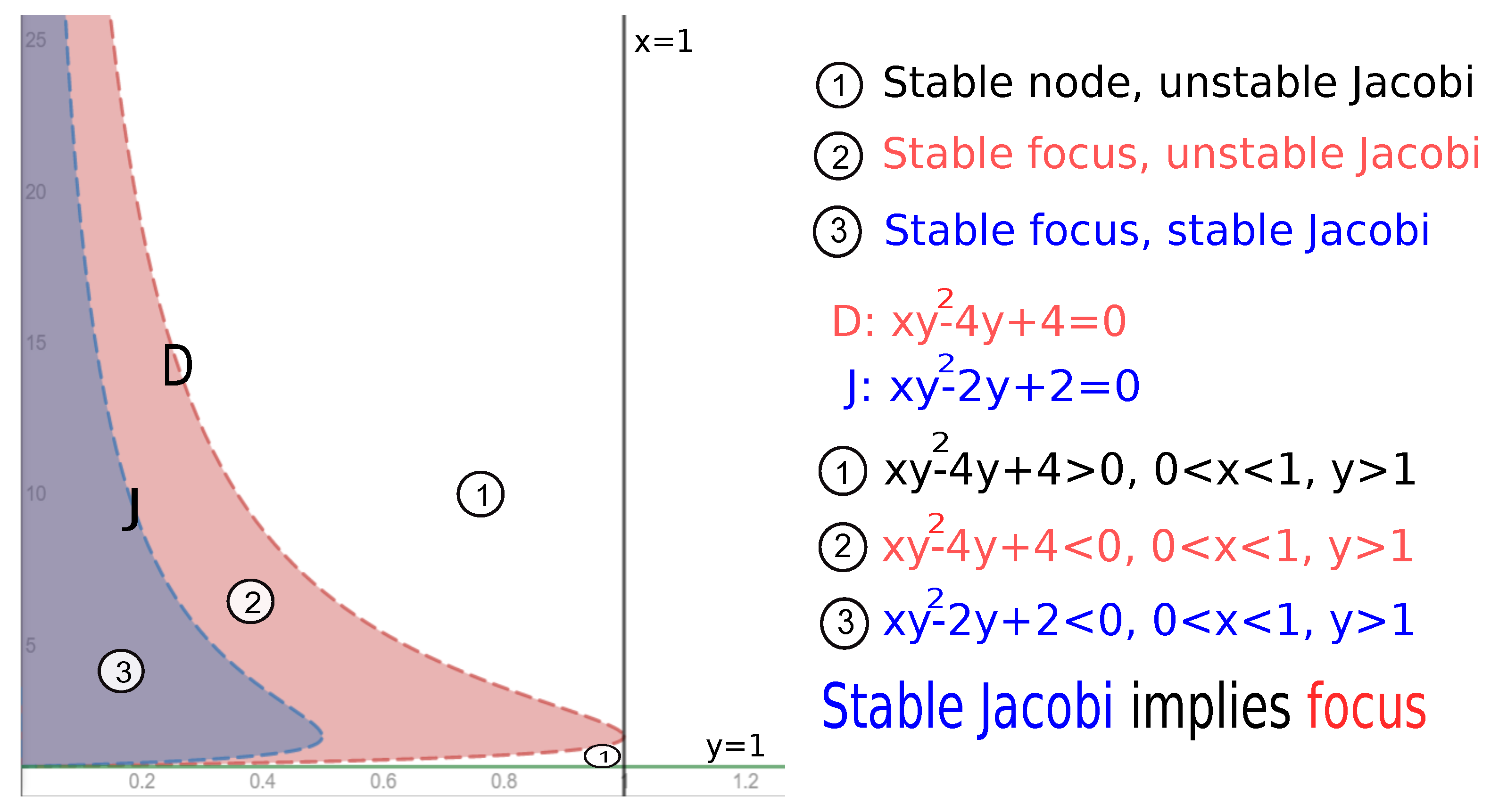

Table 1.
The equilibrium points in the closed positive quadrant for the classical SIR model.
| Case | Conditions | Equilibrium points type |
|---|---|---|
| 1 | , | saddle point, stable node |
| 2 | , | saddle point, stable focus |
| 3 | non hyperbolic | |
| 4 | stable node, |
Table 2.
The equilibrium points in the closed positive quadrant for the modified SIR model.
| Case | Conditions | Equilibrium points type |
|---|---|---|
| 1 | saddle point, , attractor or repeller | |
| 2 | , | non hyperbolic, attractor or repeller |
| 3 | , | non hyperbolic |
| 4 | , | non hyperbolic, |
| 5 | stable node, saddle point, attractor or repeller | |
| 6 | stable node, non hyperbolic, | |
| 7 | stable node, , don’t exists |
Disclaimer/Publisher’s Note: The statements, opinions and data contained in all publications are solely those of the individual author(s) and contributor(s) and not of MDPI and/or the editor(s). MDPI and/or the editor(s) disclaim responsibility for any injury to people or property resulting from any ideas, methods, instructions or products referred to in the content. |
© 2023 by the authors. Licensee MDPI, Basel, Switzerland. This article is an open access article distributed under the terms and conditions of the Creative Commons Attribution (CC BY) license (http://creativecommons.org/licenses/by/4.0/).
Copyright: This open access article is published under a Creative Commons CC BY 4.0 license, which permit the free download, distribution, and reuse, provided that the author and preprint are cited in any reuse.


