
Submitted:
14 April 2023
Posted:
14 April 2023
You are already at the latest version
Abstract
Remanufacturing is a way for product recovery initiative and maintaining sufficient production flow to satisfy customer demand through circular economy. Recently, manufacturers have been progressively incorporating remanufacturing processes, making their supply chain vulnerable to disruptions. Among the disruptions that usually occur is the shortage in spare parts supply, which causes unexpected delay in production and possible loss of sales. In the face of potential disruption, it is essential for remanufacturing facilities to manage their supply chains in an optimum manner as to decrease the adverse impact of disruptions to their business. In this study, a two-stage production-inventory system is analysed by developing a cost-minimisation model focusing on the recovery schedule after a disruption occurrence in sourcing spare parts for a remanufacturer’s production cycle. The developed model was solved using the branch and bound algorithm. Through numerical experiments, the results indicate that the optimal recovery schedule and the number of recovery cycles are significantly dependant on disruption time, lost sales and backorder costs. Moreover, a sensitivity analysis shows that the lost sales option seems to be more effective than the backorder option in optimising the system’s overall cost. The proposed model could assist managers in deciding the optimal production strategy while providing interesting managerial insights into vital spare parts recovery issues when disruption strikes.
Keywords:
Remanufacturing
; Spare Parts
; Recovery
; Disruption
; Lot size
1. Introduction
Remanufacturing is well known for its efficiency in closing the material flow loop, eliminating production waste, enhancing product life cycles, conserving energy and minimising processing costs [1,2]. Remanufacturing can be described as a method of returning used products to the state of new products which involves collecting, inspecting, disassembling, cleaning, separating, repairing and assembling [3,4]. It has been practised in a broad range of production industries, especially in the electronics and automotive sectors. Due to increased government legislation, social pressure and economic prospects, many companies have become involved in the remanufacturing industry. In addition, remanufacturing has arguably received more attention than traditional manufacturing operations due to its lower energy or resource consumption, besides acting as an incredibly less environmentally harmful approach than other processes, such as recycling or manufacturing. Supply chain disruption mitigation and recovery by Darom et al. [5] discussed the relationship between supply chain mitigation and recovery activities and their effect on environmental performance to assess the value of incorporating both entities.
However, the management of remanufacturing systems, particularly inventory plans, has always been a complicated task due to growing interactions between various manufacturing and remanufacturing operations and uncertainty in its supply chain’s various stages. The increasing need for remanufacturing due to resource scarcity, environmental deterioration and new regulations requires companies to organise their actions to explore and reap the full benefits of the coordination of forward and reverse material flows. Leuveano et al. [6] studied the inventory replenishment system in transportation and quality problems with consideration to the just-in-time (JIT) method. In addition, uncertainty in remanufacturing will subsequently cause un-expected problems related to production planning, inventory management, network design and vehicle routing [7]. However, the most common difficulties faced in the remanufacturing sector are primarily related to material flow and time control constraints in the production process [8,9,10,11].
Capacity planning in the reverse field, however, poses the following problems: somewhat uncertain market patterns, variability in the residence time of goods (the period a product lasts with its user until end of use), dependence on the quantity and timing of the end-of-use commodity returns on production and pricing patterns, and uncertainty about the amount and timing of remanufactured product returns [12,13]. These specific features include a higher risk of shortages in end-of-use product returns, since production can differ, and the dismantling level may be less than expected. This contributes to the overcapacity phenomena in selection and remanufacturing efficiency [14]. Additionally, spare parts limitations also contribute to uncertainty in remanufacturing flows. Uncertainty in the processing requirements of spare parts or goods manufactured in remanufacturing processes makes it impossible to extend traditional capacity planning in the reverse operations specifically.
Remanufacturing is a feasible way to extend the useful life of a finished product or its parts. Despite its environmental, financial and social benefits, remanufacturing is correlated with many core problems linked to availability, scheduling and consistency (the used product or its parts). Regarding environmental preservation, Ghadimi et al. [15] practised the decision-making approach for suppliers in automotive spare parts as initiatives in adopting sustainability in supply chain management. Furthermore, Shi [16] established stochastic dynamic programs to solve the spare parts inventory control problem, where a sufficient supply of remanufactured parts was satisfied with the return of products. The interrelationships among installed bases, product returns and demand for spare parts contribute to optimal demand.
Spare parts availability is one of the main components in remanufacturing. Sourcing is difficult after spare parts production declines, while the rest of the operation remains long. Kurilova-Palisaitiene et al. [17] extensively discussed the contribution of lean production to shorter lead times. Spengler et al. [18] established policies of part recovery and spare parts supply for closed loop supply chain (CLSC) by developing a generic system dynamic model providing causes and effects in various forms of product take-back. Additionally, Ronzoni et al. [19] thoroughly investigated the aftermarket distribution channel for spare parts manage-ment when they developed a model considering the supply chain for automotive spare parts after the consumer distribution channel. Additionally, Inderfurth et al. [20] recognised a problem in the automotive industry during the end-of-life (EOL) regarding spare parts procurement. They designed a stochastic dynamic programming problem with different alternatives so that total expected costs for inventory holding, shortage and purchasing can be minimised. The study by Mohapatra et al. [21] is concerned with inventory control for a remanufacturing system in which stationary demand is met by both remanufactured and newly purchased products. The model assumes that customer return products are remanufactured at a constant rate and the economic order quantity (EOQ) for manufactured and remanufactured items is computed at the same time.
Even though the above papers widely discussed overall cost reduction for spare parts, none of them explored the effect of spare parts disruption on manufacturing and remanufacturing processes in a single framework. Therefore, motivated by a case study of uncertainty in sourcing spare parts confronted by a remanufacturing company, the present paper aims to resolve this gap by developing an optimisation model focusing on the recovery schedule formulation by reducing total costs, TC, for a remanufacturer’s production cycle that is affected by disruption during spare parts collection. In this paper, we propose a cost minimisation strategy by developing a mathematical model for a CLSC recovery schedule, which consists of a combination of production cycles for new production items and remanufactured items. The recovery schedule is determined when spare parts collection is disrupted, affecting the remanufacturing cycles. The disruption stops once production and remanufacturing cycles return to normal. The main contribution of this study is the development of an efficient rescheduling mechanism to reduce total recovery costs as to fulfil the demand for the remanufactured product when faced with an uncertain spare parts collection, with consideration of mixed backorders and lost sales.
The remainder of the paper is organised as follows. The model development is presented in section 2. The results and discussions from the application of the model based on the numerical tests are elaborated in section 3. A detailed sensitivity analysis is presented in section 4. Lastly, section 5 presents concluding remarks, as well as directions for future research in this area.
2. Model Development
In this study, we examine a remanufacturing system whose inventory cycles recover after a spare parts supplier is unexpectedly disrupted. In the following sub-section, the description of the model development is discussed in detail, followed by the formulation of a mathematical model for optimal cost recovery of the inventory system under study.
2.1. Problem Description
We consider a two-stage production-inventory system that consists of a serviceable inventory (remanufacturing inventory cycle and normal production inventory cycle) and spare parts inventory. The manufacturer alternates two types of production processes, which are a remanufacturing cycle and a normal production cycle, as shown in Figure 1. The serviceable stock is a combination of new products and remanufactured products, which are able to satisfy market demand. The re-manufacturing cycles begin by receiving spare parts from the supplier, followed by the production of new manufactured items.
Spare parts collection is disrupted, unable to satisfy the requirements of the remanufacturing process, and disturbs the normal remanufacturing production cycle. The recovery period begins as soon as the disruption occurs. Since the collection quantity of the spare parts during the disruption is less than the demand of remanufactured production during regular cycles, the production of remanufacturing items is lower than its usual output. At this point, some of the customer demand cannot be fulfilled within the disruption time and be-comes backorders and lost sales. These recovery cycles continue until production returns to a normal schedule and customer demand can be fulfilled within a short time while minimising manufacturer loss.
The disruption may strike at any moment and anywhere in the production of new manufactured and remanufactured products. It may lead to changes in the behaviour of production flows to the inventory. We assume that disruption occurs in the first remanufacturing cycle, when the arrival of a spare part does not meet the requirement for the remanufacturing process. This paper addresses the cost minimalization of recovery cycles so that the manufacturer can prevent a more significant total loss during disruption. By setting Td as the disruption period, we assume that disruption occurs in spare parts collection, before the remanufacturing cycle. Spare parts are collected depending on the demand of the remanufacturing process. Since the disturbance occurs during spare parts collection, the new quantity of spare parts, Si, is less than normal spare parts ordering quantity lot size, Qs. Then, it affects the quantity production of the remanufactured product, X1, which is less than the normal remanufacturing production, Qr. The recovery cycle occurs in the next cycles, and the recovery window duration is defined as the number of recoveries, n, and the recovery window ends when the production of the remanufactured item and manufactured item return to their original schedule. Although disruption occurs, recovery in the normal manufacturer period (Tp) does not affect the production of a newly manufactured item and merely disturbs the production cycle of the remanufatured item.
2.2. Assumptions and Notations
The following assumptions have been used in the development of the recovery model:
- The demand is deterministic;
- The ordering rate of a spare part depends on the demand of the remanufacturing system;
- Disruption occurs when the suppliers cannot provide the requirement of spare parts to the remanufacturing process;
- The production rate of the new product is constant during the recovery period;
- The ordering lot of spare parts is constant during disruption;
- Lost sales and backorders occur during the recovery period;
- During recovery, one recovery cycle is recovery for both the remanufacturing and normal production cycles.
The main objective of this study is to develop a mathematical model decision support system for remanufacturing supply chain inventory management taking into account disruptions. The decision variables include Xi as the remanufacturing quantity for the recovery cycle, TXi as the time taken for the remanufacturing cycle in the recovery window and Qs as the spare part economic ordering lot size.
The following notation are used in the model cost function development:
T: length of production and remanufacturing process cycle (year)
B: unit backorder cost per unit time ($/unit/year)
L: Lost sale cost per unit ($/unit)
The following denotes the serviceable manufacturer’s parameters:
Qr: remanufacturing lot size in the original schedule (unit)
Qp: production lot size in the original schedule (unit)
Tr: remanufacturing cycle time (year)
Ts: shortage period when disruption occurs (year)
Tp: normal production cycle time (year)
Td: disruption period (year)
st: production setup time (year)
hp: holding cost per unit cost of serviceable stock ($/unit/year)
Xi: recovery for remanufacturing lot size in cycle i (i ≥ 1) (unit)
TXi: remanufacturing period in recovery cycle i (i ≥ 1) (year)
R: remanufacturing rate (unit/year)
P: normal production rate (unit/year)
Ap: normal production set up cost ($/batch)
Ar: remanufacturing setup cost ($/batch)
B: unit backorder cost per unit time
The following denotes the spare parts manufacturer’s parameters:
Qs: spare parts ordering lot size (unit)
Si: spare parts recovery ordering lot size in cycle i (i ≥ 1) (unit)
Ts: spare parts manufacturer ordering cycle time (year)
Ti: spare parts recovery period during a disruption in a cycle i (i ≥ 1) (year)
hs: holding cost per unit cost of spare parts stock ($/unit/year)
C: spare parts collection rate (unit/year)
DR: demand rate of spare part use (unit/year)
2.3. Mathematical Formulation
The optimal lot size for Qp and Qr and Tp, and Tr for the above ideal system is formulated based on the original work by Mohapatra et al. [21]as follows:
For this model, we consider four main costs in the recovery cycles. The first one is set up cost (TC1), which is rather straight forward as:
Next, the total cost for inventory holding cost (TC2) is a derivation of multiplying the unit inventory holding cost by the total inventory during the recovery cycle. Let hs and hp represent the holding cost per unit cost of spare parts and the serviceable stock, respectively. The spare part inventory (TC21) is expressed as follows:
where
Substituting Equation (7) for Equation (6), we get
The holding cost for serviceable inventory (TC22) is expressed as follows:
where
By inserting Equation (10) into Equation (9), we get
Substituting , we obtain
The total holding cost can be expressed as:
Therefore, by replacing Equation (8) and Equation (12) with Equation (13), the following function for total holding costs is obtained:
Next is the total backorder cost (TC3) formulation, which is the product of the unit backorder cost, B, with the backorder quantity of each cycle, Xi, and delay time, Delayi (22),(23). The formulation can be derived as follows:
Delayi is derived for each cycle. Delayn is the time delay for the cycle, n. Delayi is calculated as below:
For the first cycle, n = 1, there is no time delay for the delivery of the spare parts collection for the remanufacturing process.
n = 1; no delay,
For n = 2,
n =3,
n = 4,
Therefore, the total Delayi can be expressed as
By substituting Equation (15) for Equation (14), the backorder cost results:
Lastly, the total lost sale cost (TC4) is expressed as
Adding the total cost, TC expressions above gives the overall total cost of recovery. Therefore, the mathematical model for the problem is presented as follows:
Subject to the constraints
All decision variables are nonnegative
The objective function (18) for minimising the TC takes into consideration the setup cost, holding cost, backorder cost and lost sale cost. Equations (19) and (20) certify that the production of remanufacturing during the recovery schedule does not exceed regular remanufacturing production due to disruption in spare parts collection. Equation (21) ensures that demand is fulfilled within a period of time, while Equation (22) is serviceable production capacity constraint. All decision variables need to be in positive values. By solving the developed model for Xi, Si and n, an optimal recovery plan with a minimal TC can be obtained even for systems under disruption.
3. Numerical Analysis
Various experiments are discussed in this section, demonstrating the applicability and efficiency of the proposed model and method. The mathematical model presented in this paper is categorised as a nonlinear constrained quadratic programming problem and has been solved using the branch and bound algorithm.
The basic parameters used in this model or benchmark parameter are defined as test problem 1 as tabulated in Table 1. The holding cost value, hp and hs, and the rate for production, remanufacturing and demand, P, R, and DR, respectively, were adapted from [8]; the other parameters are based on the assumptions deemed suitable for the developed model. The developed model was then tested with multiple sets of parameters to ensure that valid and credible output was generated. In Table 2, test problem 2 provides pattern behaviour of the remanufacturing setup cost when increased. For test problem 3 and 4, the holding cost for the serviceable stock and spare parts were doubled, respectively. The disruption time was increased to 0.04 s in test problem 5. The result was graphically illustrated in Figure 2, as the plot shows a convex curve, implying that the model and solution procedure established in this paper provides good solutions.
4. Sensitivity Analysis
In this section, a sensitivity analysis is conducted to analyse the impact of system efficiency on analysing the optimal TC values with various data sets. To perform the sensitivity analysis, we run the same experiment with precisely the same parameters and characteristics but with a different setup cost, unit inventory holding cost, backorder cost, lost sale cost and disruption time. All the other parameters, if not varied, remain unchanged based on the data set for test problem 1.
The setup cost for remanufacturing and production was increased from 50 to 350 and was tested using the test problem data set, as shown in Figure 3. The plotted graph shows that the TC is directly proportional to the production and remanufacturing setup costs. Since the setup cost is one of the components that has been considered in the developed model, increments in setup cost will increase the overall TC. The unit inventory holding cost in the mathematical model is the holding cost for serviceable and spare parts stock. Figure 4 displays the results of the TC with the increment in the unit inventory holding cost when using test problem 1 parameters. The other parameters remain unchanged, except for the total holding cost value for the serviceable and spare parts stock. For this test, it is shown that when hs is increased, the total cost also increases. However, the increment in hp will drop the TC value. This is due to the relationships between Qr, Qp and hp based on equation (1) and (2). The value for Qr and Qp act inversely proportional to the hp value. As the hp increases, the Qr and Qp decreases, as does the TC.
Figure 5 depicts the results derived from the tests conducted for the relationship between the backorder unit cost and the backorder cost, TC and n. The plotted graph shows that the backorder cost increases as the backorder unit cost increases. Similarly, the TC behaviour also increases when the backorder unit rises. However, the optimal number of cycles decreases from n=3 to n=2 as the backorder unit cost increases. This occurs due to the increment of the backorder, which is less cost-effective than lost sales during the recovery schedule. Hence, the lost sale cost affects the overall TC and the unmet demand becomes lost sales. At the same time, the quantity production of the serviceable item is reduced, leading to a shorter recovery time.
The effect of changing Td on the TC and lost sales cost is depicted in Figure 6. One can argue that the TC depends on the changes in Td. It can be noticed that the minimum value of TC decreases at n= 3 until Td reaches 0.045. Conversely, TC sharply increases at 5% after Td is more than 0.045 and the TC achieves a maximum value when n= 2. Thus, as Td increases, the affected remanufacturing cycle’s quantity is less than its regular schedule, and the unfulfilled quantity of demand also escalates, thus influencing the lost sales cost. This results in additional costs to the TC. Hence, the recovery method is optimal only until a certain Td, after which a backup supplier might be a better option. It is important to determine a recovery option for the manufacturer to overcome additional TC to cut company loss.
5. Case Study
After various tests were conducted on the developed model, a real case study was performed to validate the mathematical model. Among the advantages of real case studies is being able to explain the complexity of real situations that may not be obtained through simulations, experiments or surveys by detailing data in a real-life environment [22]. Therefore, data from selected industries were obtained to implement the actual case study method. The selected company, Company A, has agreed to allow the shared data to be used in this study.
5.1. Company overview
Company A is an industry that provides repair services for heavy machinery vehicles, especially prime movers. According to the records provided, there are more than 30 prime movers all over Malaysia’s east coast that get repair services from this company. The repair cases carried out at this company are related to the engine system, brake system, lubrication system and transmission system.
For the actual study of the development of this model, the transmission system was chosen because according to an interview with the company, the percentage of obtaining spare parts during the overhaul of the transmission system is high. Therefore, the study on transmission system spare parts is explained in more detail for the next sub-section.
The developed model mainly aims to reduce the cost of recovery that companies have to bear when disruptions occur. The most significant disruption experienced by most companies in the past year was related to the pandemic that was sweeping the world, namely Covid-19 [23]. However, the first case in Malaysia was detected in January 2020 and the Covid-19 cases became more contagious. Following the sudden increase in cases, the government decided to implement a movement control order (MCO) in March 2020. Consequently, the Malaysian economy suffered a severe collapse and affected the income of most sectors.
Company A was also affected when the MCO was implemented throughout Malaysia. The highest repair frequency in the company is the brake system followed by the lubrication system and the transmission system. However, spare parts for the brake system are readily available and the company does not face difficulties in the process of overhauling the brake system.
The data provided is related to the replacement process of the clutch component in the transmission system which is the Clutch Servo Pump (Figure 7). These components are supplied by the main supplier of spare parts, which is Supplier V located in Kuala Lumpur, Federal Territory.
5.2. Model Validation and Discussion
The study on the transmission system spare parts was conducted by using the data obtained from the industry, as stated in Table 3, which is for the case when a disruption occured.
LINGO software was usedto solve the case study data, where the optimal TC was identified as in Table 4. As the turnaround cycle increases, the optimal cost of TC also increases due to increased setup costs, although the optimal TC value occurred at n = 3 due to the balance of the cost of delayed orders, TC3, and the cost of lost sales, TC4. Note that the TC calculation in the table below is for a specific period only. However, if this cost continues, it is feared that it could affect the company's annual income.
The company takes effective mitigation measures to reduce the negative impact especially on the company's finances from bankruptcy. Among the measures taken by this company is to obtain spare parts supply from backup suppliers or second suppliers. Based on the interviews that was held, the company stated that the costs the company had to bear may exceed the annual budget for production costs, but it was enough to save the company's economy to continue operating.
The company has several back-up suppliers who may be able to supply spare parts requirements. It consists of Supplier W (Perak), Supplier X (Kelantan), Supplier Y (Perak), and Supplier Z (Terengganu). Nevertheless, the selection to obtain spare parts is based on the cost per unit of spare parts and also the length of time taken by the supplier to provide the spare parts as requested. In addition, the level of availability of spare parts is very important for manufacturers in planning the company's production strategy. Figure 8 below shows the relationship between manufacturers in deciding the decision to obtain spare parts from the suppliers that have been mentioned. Location is also an important factor in the selection of spare parts suppliers as location selection may significantly reduce delivery or purchase time and can reduce the risk of disruption.
Nevertheless, the level of readiness or availability also plays an important role in the selection of suppliers. The higher the percentage of spare parts availability, the more attractive the manufacturer is to obtain supplies from suppliers. For example, Supplier Z is the supplier that has the least distance with the Company A but the level of availability of spare parts is the lowest and it is possible that the required spare parts are unavailable and require a longer period of time to fulfill the order or are sold at a higher price. This is usually the case when customers have not much choice and desperately need spare parts.
Figure 9 shows a comparison of unit prices for spare parts between suppliers. Supplier V offers the lowest price per unit of spare parts compared to theother suppliers. Supplier Z recorded the highest price even though it was the closest to Company A. This is due to the limited number of spare parts suppliers around the area which in turn gives these suppliers the opportunity to raise prices. Although Supplier W has a high percentage of spare parts provision, the supply of spare parts for Clutch Servo Pump could not be fulfilled due to internal problems faced by the company. Therefore, the preparation period is considerably long despite the low and attractive price offered.
The comparison between spare parts preparation period and recovery TC is further elaborated in Figure 10. During the disruption, the Supplier Y recorded the lowest TC value when compared to other suppliers. Although the unit price of RM 570 is the same as the unit price of spare parts from Supplier X, the disurption period, Td, for Supplier X is 0.001 which affects the overall TC to repair the transmission system. If seen from the behavior of the line graph that shows the preparation period by each supplier during the disruption, Supplier Y and Supplier Z can supply spare parts directly to Company A but the difference in cost per unit causes a gap between the recovery TC for these two suppliers.
In conclusion, several factors such as the price per unit cost of spare parts, preparation period and total recovery costs influence the manufacturer's decision to make the right choice in dealing with the disruption event. It is recommeneded for the management to analyze the entire total costs involved during the disruption and its impact on the company's economy either for the current period or for the long term. The management may also evaluate the characteristics of a quality backup supplier by evaluating the current issues faced by the management, taking into account the optimal total costs as suggested by the model by evaluating the different cost component allocations from the supplier.
6. Managerial Implications
This study analyses the impact of parts supply disruptions on the remanufacturing industry. The management may take several mitigation measures to reduce the negative impact on the company, especially in terms of the company's economy and reputation. The disclosure of the cost components involved in the calculation of total recovery costs can provide an early insight to the management in dealing with issues related to the company's expenses in the event of disruptions. In order to reduce recovery costs, back-up suppliers can be considered to reduce the manufacturing period and meet customer demand in a timely manner. It is also important for the management to know the economic status of their supply chain system as a whole to reduce the negative implications of the company in the long run.
Among other mitigation measures that can be implemented by the management is to obtain the supply of spare parts from different suppliers by comparing the price per unit of spare parts components, the level of availability and the time period for them to be obtained. In addition, incorporating optimisation methods is essentially important for decision-making in the remanufacturing sector which will help managers to make sound decisions when faced with the various process complexities and uncertainties [24]. Utilising optimisation techniques such as the developed model can further aid manufacturers to determine the effects of disruption for longer periods of time, particularly when selecting backup suppliers during disruptions.
7. Conclusions
This paper presents a mathematical model that determines the recovery schedule for the remanufacturing production system after the spare parts collection cycle is disrupted. In-tending to minimise TC, we assume that only the remanufactured quantity is affected after disruption, while the quantity for the normal manufactured item remains constant. The solution of the developed model not only minimises the overall TC but also helps to optimise the quantity for each remanufacturing cycle during the recovery schedule such that recovery duration is minimised. The model was solved as a nonlinear quadratic programming problem using the branch and bound algorithm.
The results show that parameters such as the remanufacturing holding cost, lost sale cost and backorder unit cost influence the model’s total recovery cost. The disruption time parameter is also significant in contributing to the change in the optimal TC. The pattern of the solution for the serviceable item production relies significantly on the disruption period in the normal cycle. As the disruption time increases, the portion of unmet demand during the disruption cycle also rises. This behaviour contributes to the pattern of lost sales and backorder quantities. To achieve the minimal TC, the developed model will identify the optimal quantity of shortages that become either lost sales or backorders depending on the system’s recovery schedule.
This work can be expanded through the integration of certain factors. Interesting future work would consider several recovery processes (e.g., recyclable, repairable and refurbished) or a stochastic system for the recovery processes. Furthermore, future studies may investigate other environmental factors, such as carbon dioxide emission and energy usage, to improve sustainability goals in the remanufacturing industry.
Author Contributions
Conceptualization, N.M.R. and H.H.; methodology, N.M.R. and H.H.; software, N.M.R. and H.H.; validation, N.M.R., H.H., and D.A.W.; formal analysis, N.M.R. and H.H.; investigation, N.M.R. and H.H.; resources, H.H.; data curation, N.M.R. and H.H.; writing—original draft preparation, N.M.R. and H.H.; writing—review and editing, H.H., W.A.J., N.K.K. and F.A.A.R.; visualization, N.M.R. and H.H.; supervision, H.H., D.A.W.; project administration, N.M.R. and H.H.; funding acquisition, M.R.A.M., I.F.M., M.A.M.S. All authors have read and agreed to the published version of the manuscript.
Funding
This research was funded by the Ministry of Higher Education, Malaysia under the Konsortium Kecemerlangan Penyelidikan Grant (Grant Number: KKP/2020/UKM-UKM/2/1).
Data Availability Statement
Not applicable.
Acknowledgments
The authors would like to thank the Ministry of Higher Education, Malaysia for supporting this research with Konsortium Kecemerlangan Penyelidikan Grant (Grant Number: KKP/2020/UKM-UKM/2/1).
Conflicts of Interest
The authors declare no conflict of interest.
References
- Yang, S.S.; Ngiam, H.Y.; Ong, S.K.; Nee, A.Y.C. The Impact of Automotive Product Remanufacturing on Environmental Performance. Procedia CIRP 2015, 29, 774–779. [Google Scholar] [CrossRef]
- Amelia, L.; Wahab, D.A.; Haron, C.H.C.; Muhamad, N.; Azhari, C.H. Initiating Automotive Component Reuse in Malaysia. J. Clean. Prod. 2009, 17, 1572–1579. [Google Scholar] [CrossRef]
- Lalmazloumian, M.; Abdul-Kader, W.; Ahmadi, M. A Simulation Model of Economic Production and Remanufacturing System Under Uncertainty. In Proceedings of the IIE Annual Conference. Proceedings; 2014, Institute of Industrial and Systems Engineers (IISE); p. 3211.
- Gungor, A.; Gupta, S.M. Issues in Environmentally Conscious Manufacturing and Product Recovery: A Survey. Comput. Ind. Eng. 1999, 36, 811–853. [Google Scholar] [CrossRef]
- Darom, N.A.M.; Hishamuddin, H.; Ramli, R.; Nopiah, Z.M.; Sarker, R.A. Investigation of Disruption Management Practices and Environmental Impact on Malaysian Automotive Supply Chains: A Case Study Approach. J. Kejuruter. 2020, 32, 341–348. [Google Scholar] [CrossRef] [PubMed]
- Leuveano, R.A.C.; Ab Rahman, M.N.; Mahmood, W.M.F.W.; Saleh, C. Integrated Vendor-Buyer Lot-Sizing Model with Transportation and Quality Improvement Consideration under Just-in-Time Problem. Mathematics 2019, 7. [Google Scholar] [CrossRef]
- Govindan, K.; Soleimani, H.; Kannan, D. Reverse Logistics and Closed-Loop Supply Chain: A Comprehensive Review to Explore the Future. Eur. J. Oper. Res. 2015, 240, 603–626. [Google Scholar] [CrossRef]
- Giri, B.C.; Sharma, S. Optimizing a Closed-Loop Supply Chain with Manufacturing Defects and Quality Dependent Return Rate. J. Manuf. Syst. 2015, 35, 92–111. [Google Scholar] [CrossRef]
- Yusop, N.M.; Wahab, D.A.; Saibani, N. Analysis of Remanufacturing Practices in the Malaysian Automotive Industry. J. Teknol. (Sciences Eng. 2012, 59, 77–80. [Google Scholar] [CrossRef]
- Golinska, P.; Kuebler, F. The Method for Assessment of the Sustainability Maturity in Remanufacturing Companies. Procedia CIRP 2014, 15, 201–206. [Google Scholar] [CrossRef]
- Jindal, A.; Sangwan, K.S. Closed Loop Supply Chain Network Design and Optimisation Using Fuzzy Mixed Integer Linear Programming Model. Int. J. Prod. Res. 2014, 52, 4156–4173. [Google Scholar] [CrossRef]
- Georgiadis, P.; Athanasiou, E. Flexible Long-Term Capacity Planning in Closed-Loop Supply Chains with Remanufacturing. Eur. J. Oper. Res. 2013, 225, 44–58. [Google Scholar] [CrossRef]
- Geyer, R.; Van Wassenhove, L.N.; Atasu, A. The Economics of Remanufacturing under Limited Component Durability and Finite Product Life Cycles. Manage. Sci. 2007, 53, 88–100. [Google Scholar] [CrossRef]
- Fleischmann, M.; Bloemhof-Ruwaard, J.M.; Dekker, R.; Van Der Laan, E.; Van Nunen, J.A.E.E.; Van Wassenhove, L.N. Quantitative Models for Reverse Logistics: A Review. Eur. J. Oper. Res. 1997, 103, 1–17. [Google Scholar] [CrossRef]
- Ghadimi, P.; Dargi, A.; Heavey, C. Sustainable Supplier Performance Scoring Using Audition Check-List Based Fuzzy Inference System: A Case Application in Automotive Spare Part Industry. Comput. Ind. Eng. 2017, 105, 12–27. [Google Scholar] [CrossRef]
- Shi, Z. Optimal Remanufacturing and Acquisition Decisions in Warranty Service Considering Part Obsolescence. Comput. Ind. Eng. 2019, 135, 766–779. [Google Scholar] [CrossRef]
- Kurilova-Palisaitiene, J.; Sundin, E.; Poksinska, B. Remanufacturing Challenges and Possible Lean Improvements. J. Clean. Prod. 2018, 172, 3225–3236. [Google Scholar] [CrossRef]
- Spengler, T.; Schröter, M. Strategic Management of Spare Parts in Closed-Loop Supply Chains - A System Dynamics Approach. Interfaces (Providence). 2003, 33, 7–17. [Google Scholar] [CrossRef]
- Ronzoni, C.; Ferrara, A.; Grassi, A. A Stochastic Methodology for the Optimal Management of Infrequent Demand Spare Parts in the Automotive Industry. IFAC-PapersOnLine 2015, 28, 1405–1410. [Google Scholar] [CrossRef]
- Inderfurth, K.; Kleber, R. An Advanced Heuristic for Multiple-Option Spare Parts Procurement after End-of-Production. Prod. Oper. Manag. 2013, 22, 54–70. [Google Scholar] [CrossRef]
- Mohapatra, S.; Mahapatra, R.N.; Biswal, B.B.; Balabantray, B.; K. behera, A. A Deterministic Model for Remanufacturing Inventory for Reverse Supply Chain. Int. J. Eng. Technol. 2018, 7, 207–210. [Google Scholar]
- Zainal, Z. Case Study as a Research Method. J. Kemanus. 2007, 5. [Google Scholar]
- Khatib, S. F. , & Nour, A. The impact of corporate governance on firm performance during the COVID-19 pandemic: Evidence from Malaysia. Journal of Asian Finance. Economics and Business. 2021, 8, 0943–0952. [Google Scholar]
- Ropi, N. M., Hishamuddin, H., Abd Wahab, D., & Saibani, N. Optimisation Models of Remanufacturing Uncertainties in Closed-Loop Supply Chains–A Review. IEEE Access. 2021, 9, 160533–160551.
Figure 1.
The behaviour of spare parts inventory curve with disruption (above); remanufacturing and manufacturing inventory curves with recovery cycles after disruption (below).
Figure 1.
The behaviour of spare parts inventory curve with disruption (above); remanufacturing and manufacturing inventory curves with recovery cycles after disruption (below).
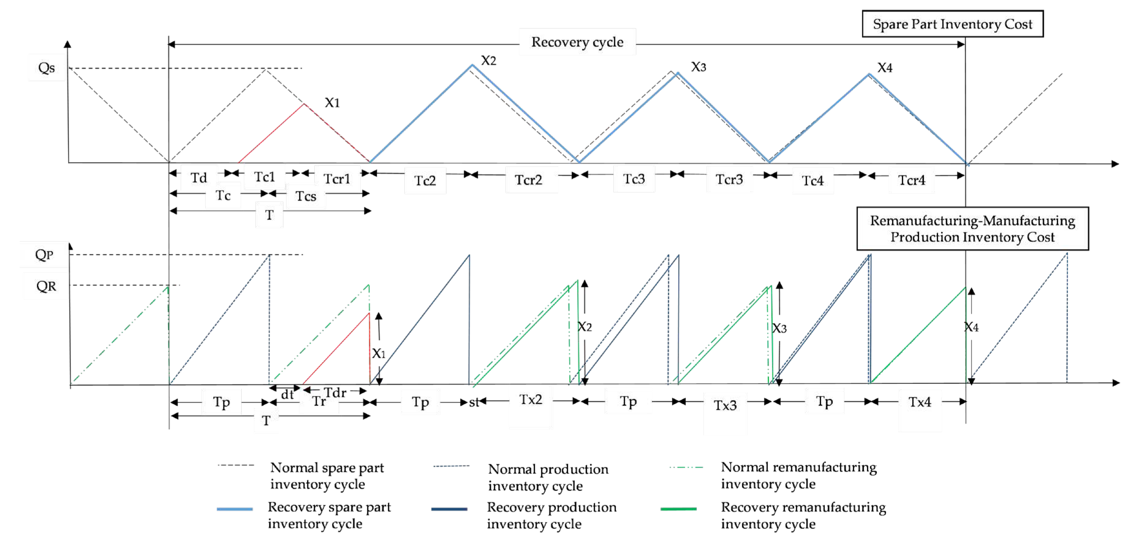
Figure 2.
TC vs n for different test problems.
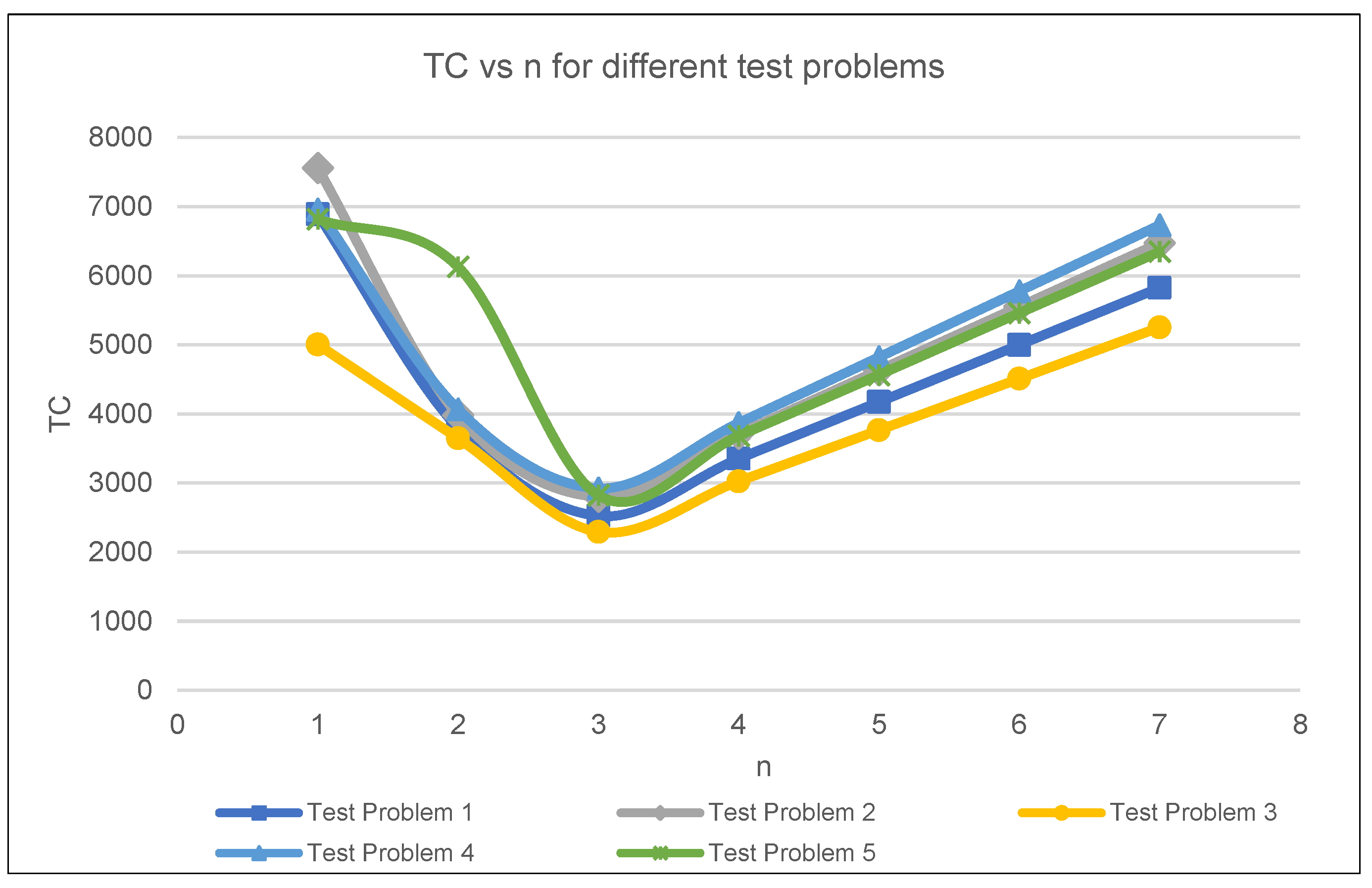
Figure 3.
TC vs Ap and Ar.
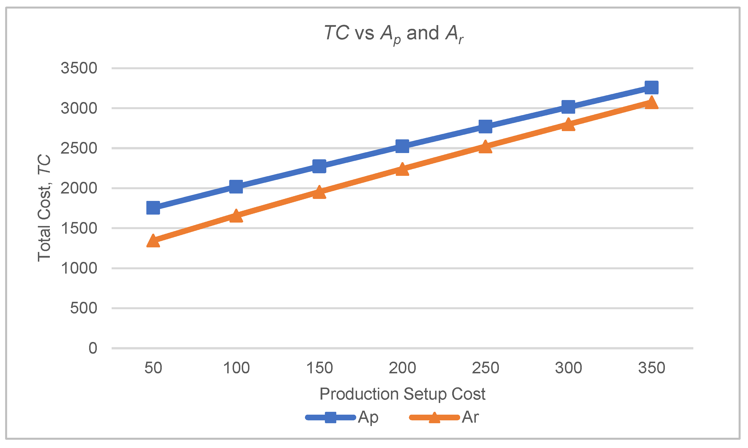
Figure 4.
Unit Inventory Holding Cost vs TC.
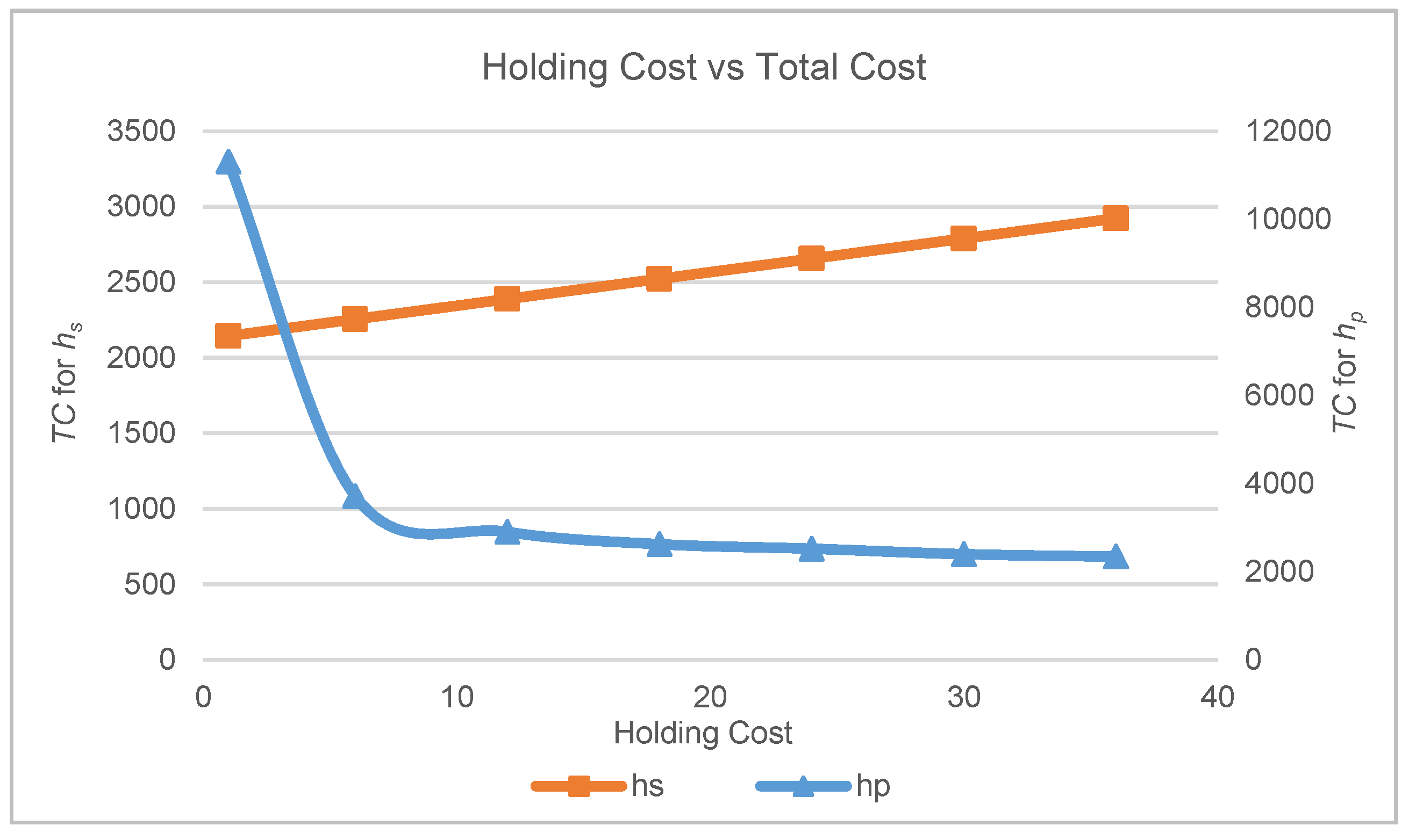
Figure 5.
Backorder cost vs TC, B, n.
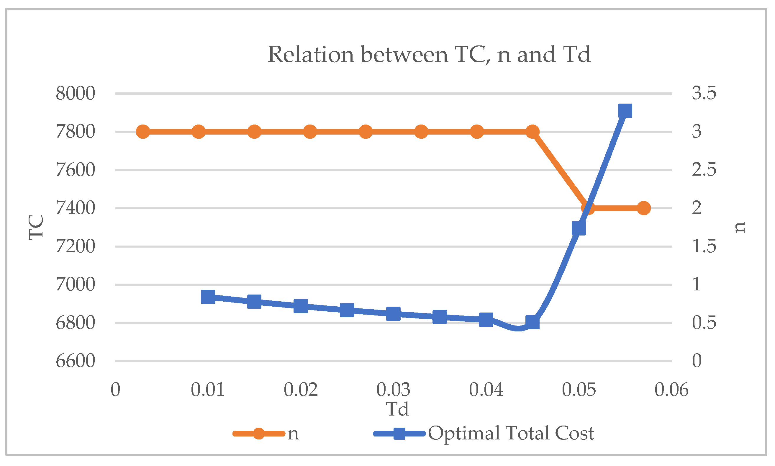
Figure 6.
Relation of optimal TC, n and Td.
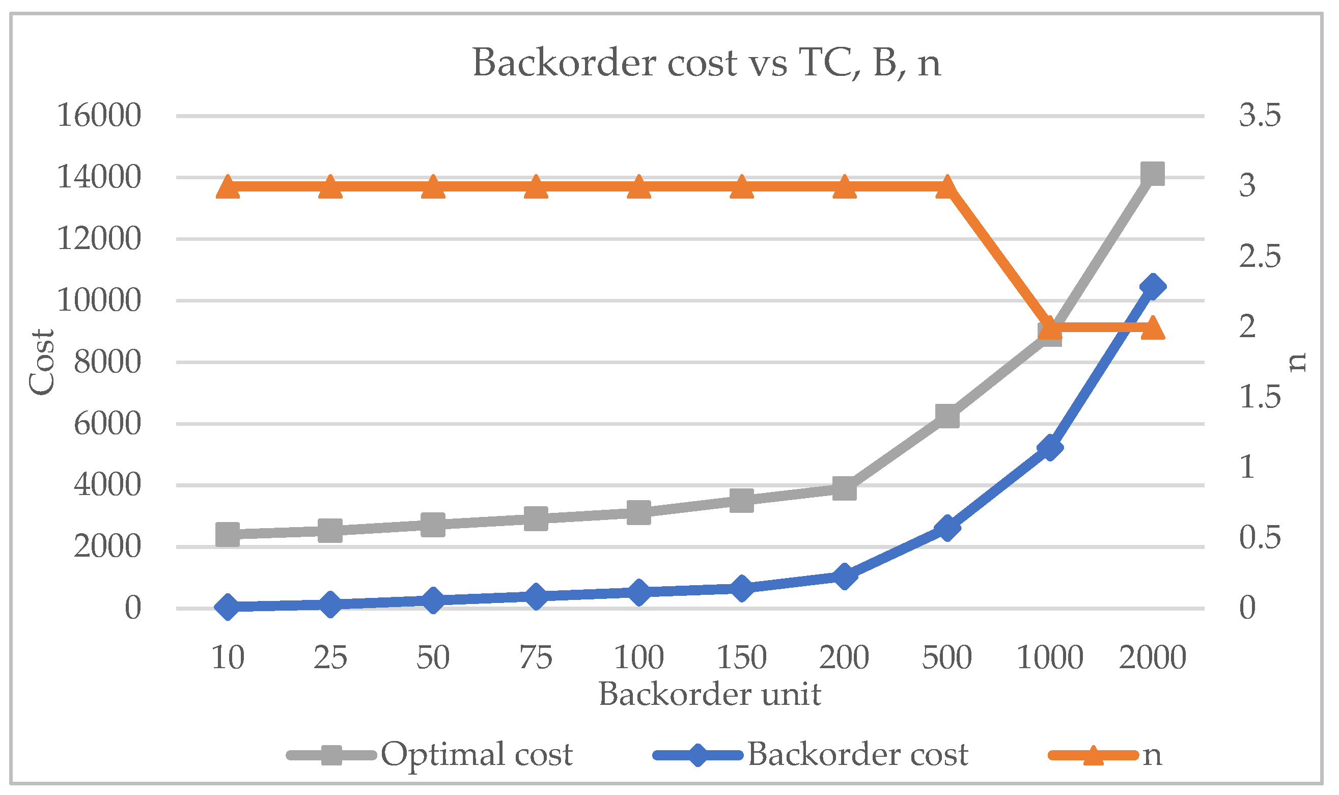
Figure 7.
Clutch Servo Pump.
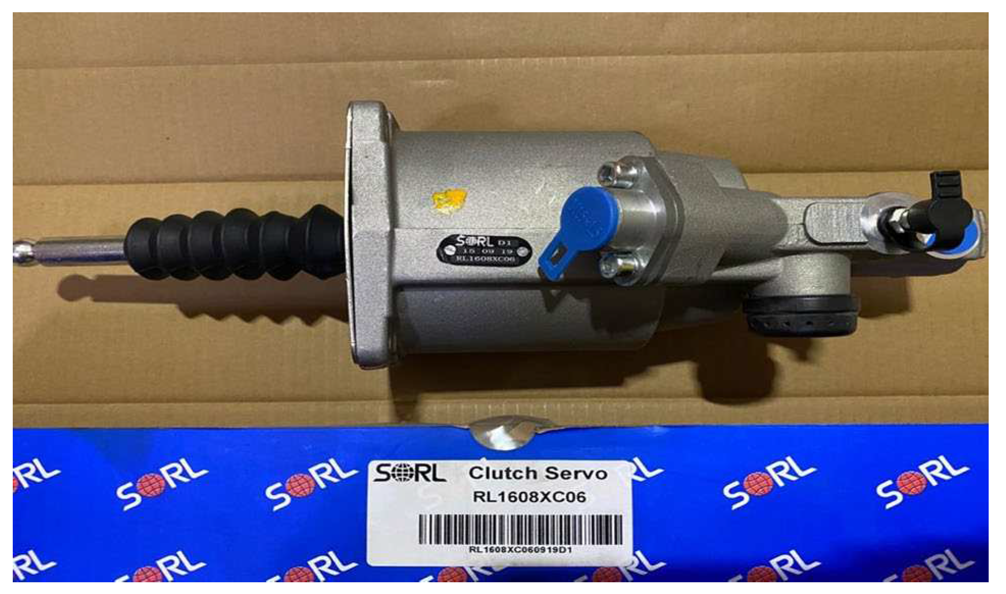
Figure 8.
Supplier selection factors.
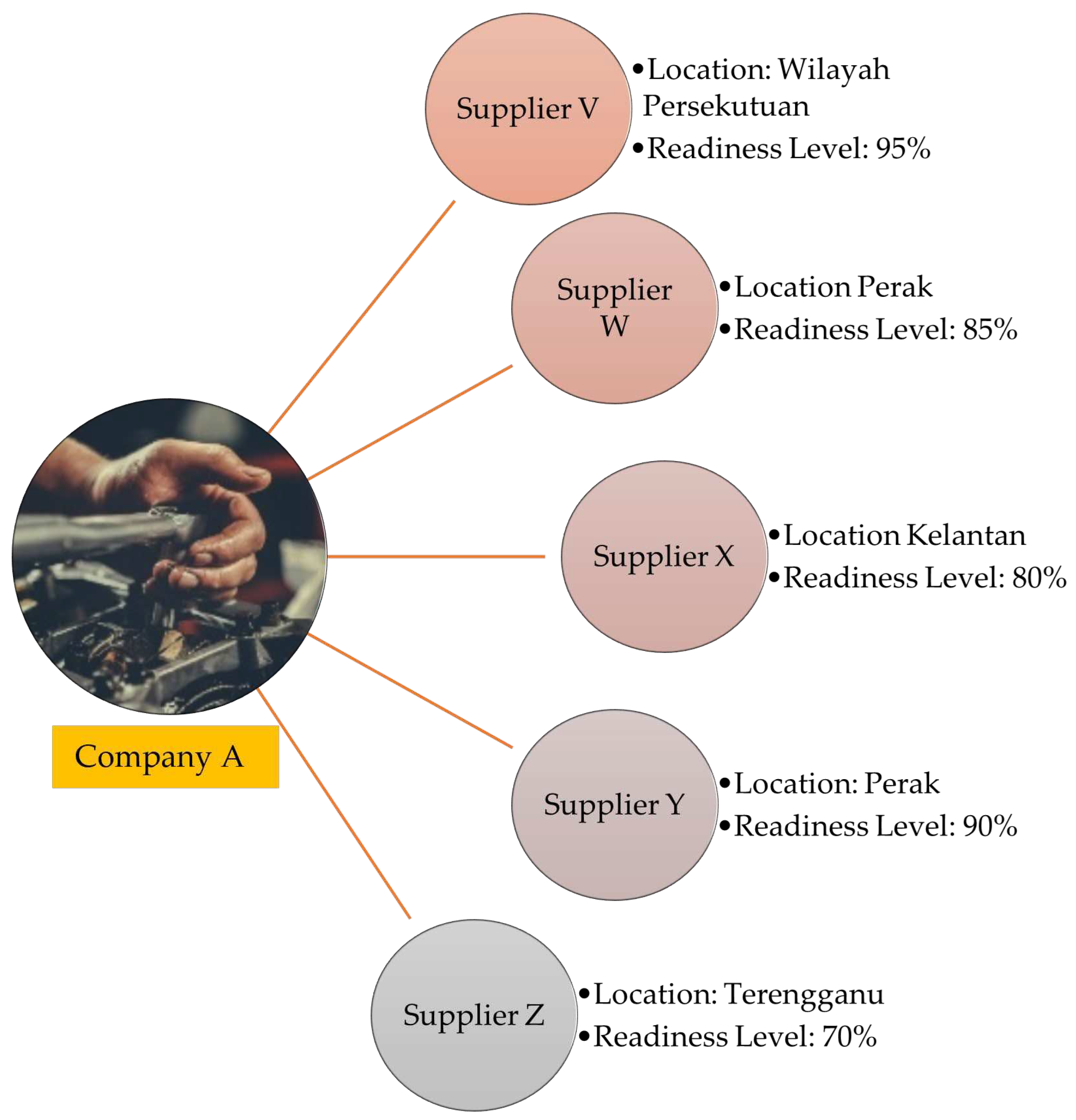
Figure 9.
Comparison of spare parts unit prices between suppliers.
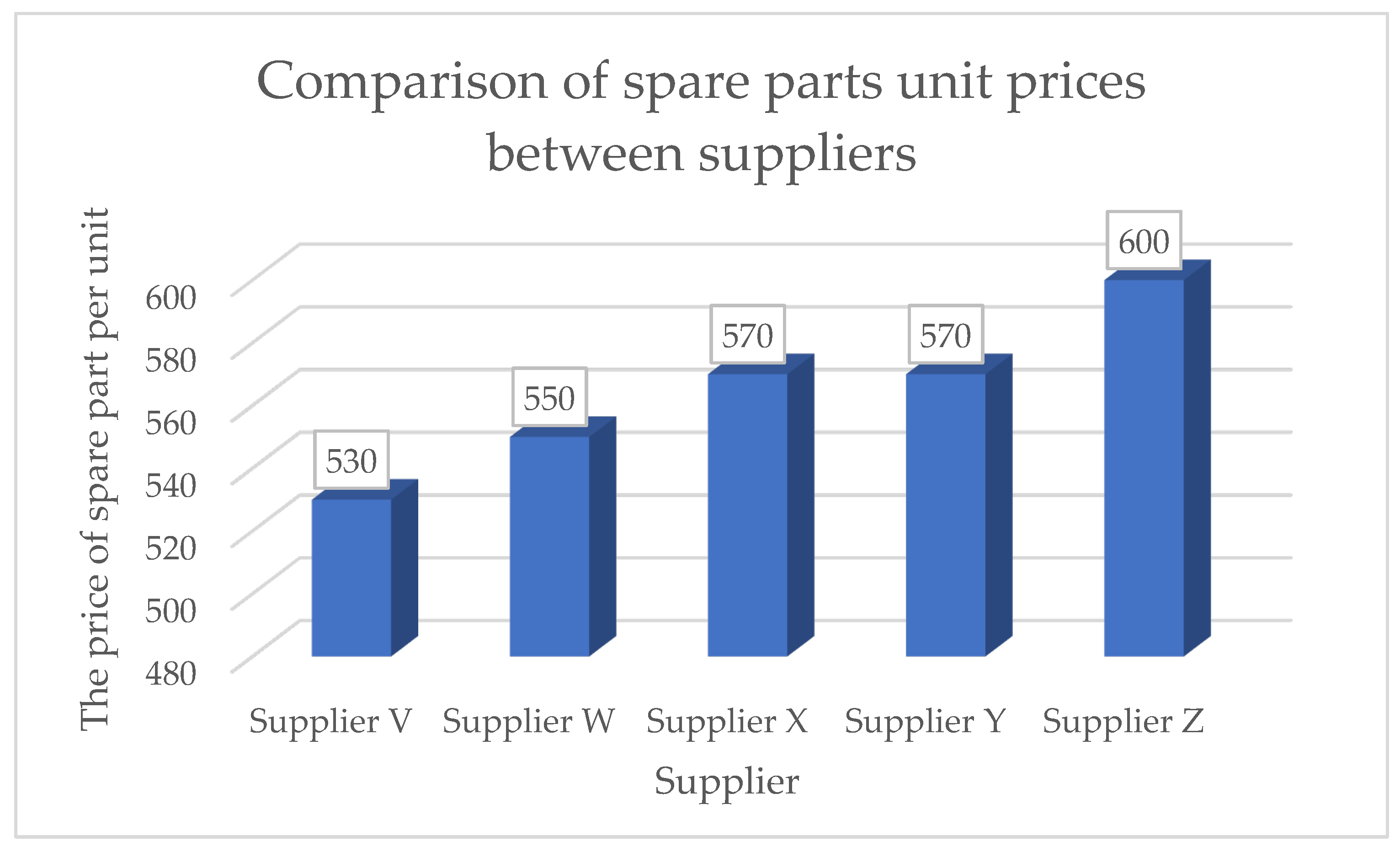
Figure 10.
Influence of Td in TC Recovery.
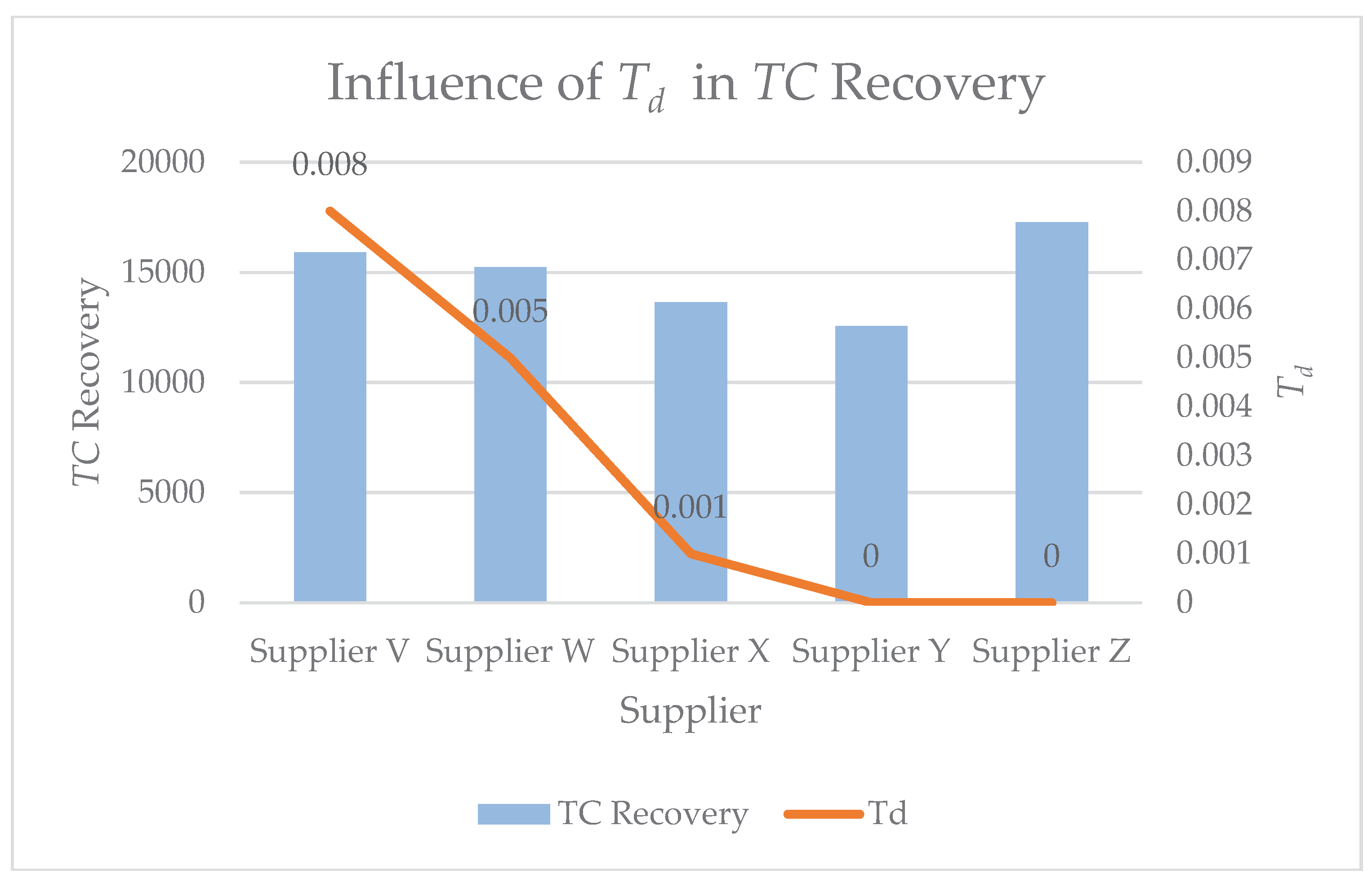

Table 1.
Set of tests with different data sets.
| Parameters | Test 1 | Test 2 | Test 3 | Test 4 | Test 5 |
|---|---|---|---|---|---|
| Ap | 200 | 200 | 200 | 200 | 200 |
| Ar | 250 | 300 | 250 | 250 | 250 |
| hp | 22 | 22 | 44 | 22 | 22 |
| hs | 18 | 18 | 18 | 36 | 18 |
| B | 25 | 25 | 25 | 25 | 25 |
| L | 50 | 50 | 50 | 50 | 50 |
| Td | 0.02 | 0.02 | 0.02 | 0.02 | 0.04 |
Table 2.
Results for the test with different data sets.
| n | Test 1 | Test 2 | Test 3 | Test 4 | Test 5 |
|---|---|---|---|---|---|
| 1 | 6887.58 | 7558.72 | 5003.73 | 6958.46 | 6816.13 |
| 2 | 3793.30 | 3978.42 | 3645.81 | 4065.64 | 6127.67 |
| 3 | 2522.31 | 2799.95 | 2922.9 | 2922.9 | 2822.09 |
| 4 | 3351.32 | 3712.84 | 3023.8 | 3867.74 | 3681.98 |
| 5 | 4171.71 | 4618.49 | 3765.05 | 4820.86 | 4564.9 |
| 6 | 4997.84 | 5551.58 | 4508.54 | 5776.05 | 5459.32 |
| 7 | 5825.42 | 6472.24 | 5252.92 | 6732.06 | 6347.98 |
Table 3.
Data obtained from the industry when the disruption occured.
| Parameter | Value |
|---|---|
| Ap | 520 |
| Ar | 650 |
| hp | 46.8 |
| hs | 57.2 |
| B | 700 |
| L | 1000 |
| Td | 0.008 |
| D | 2600 |
| R | 5200 |
| C | 5460 |
| P | 7800 |
Table 4.
Actual cost for the case study.
| n | TC1 | TC2 | TC3 | TC4 | TC |
|---|---|---|---|---|---|
| 1 | 1,170.00 | 622.45 | 0 | 41,600.00 | 43,392.45 |
| 2 | 2,340.00 | 1,471.98 | 2,136.48 | 10,944.07 | 16,892.53 |
| 3 | 3,510.00 | 2,299.86 | 6,168.66 | 3,936.10 | 15,914.62 |
| 4 | 4,680.00 | 3,443.29 | 13,450.64 | 0 | 21,573.94 |
| 5 | 5,850.00 | 4,389.72 | 20,527.84 | 0 | 30,767.56 |
| 6 | 7,020.00 | 5,455.82 | 28,608.70 | 0 | 41,084.52 |
| 7 | 8,190.00 | 6,678.45 | 37,319.96 | 0 | 52,188.41 |
Disclaimer/Publisher’s Note: The statements, opinions and data contained in all publications are solely those of the individual author(s) and contributor(s) and not of MDPI and/or the editor(s). MDPI and/or the editor(s) disclaim responsibility for any injury to people or property resulting from any ideas, methods, instructions or products referred to in the content. |
© 2023 by the authors. Licensee MDPI, Basel, Switzerland. This article is an open access article distributed under the terms and conditions of the Creative Commons Attribution (CC BY) license (http://creativecommons.org/licenses/by/4.0/).
Copyright: This open access article is published under a Creative Commons CC BY 4.0 license, which permit the free download, distribution, and reuse, provided that the author and preprint are cited in any reuse.


