Preprint
Article

Performance Analysis of Segmentation and Classification of CT scanned Ovarian Tumours using UNet and Deep Convolutional Neural Networks

Altmetrics

Downloads

228

Views

102

Comments

0

Submitted:

13 April 2023

Posted:

13 April 2023

You are already at the latest version

Alerts
Abstract
The difficulty in detecting tumors in earlier stages is the major cause of mortalities of patients, despite the advancements in treatment and research regarding ovarian cancer. Deep Learning algorithms are applied to serve the purpose of a diagnostic tool by applying them on CT scan images of the ovarian region. The images go through a series of pre-processing techniques and further the tumor is segmented using the UNet model. Instances are then classified into two categories – benign and malignant tumors. Classification is performed using Deep Learning models like CNN, ResNet, DenseNet, Inception-ResNet, VGG16 and Xception along with Machine Learning models such as Random Forest, Gradient Boosting, AdaBoosting, XGBoosting. DenseNet 121 emerges as the best model on this dataset even after applying optimization on the Machine Learning models by obtaining an accuracy of 95.7%. The current work demonstrates the comparison of multiple CNN architectures among themselves and with common Machine Learning algorithms, with and without optimization techniques applied.
Keywords: 
Subject: Computer Science and Mathematics  -   Mathematical and Computational Biology

1. Introduction

Ovarian cancer stands out as a commonly diagnosed type of cancer worldwide. Considering the fact that it usually goes unrecognised until terminal stages, ovarian cancer is a leading reason for high mortality rates among women with gynaecological illnesses. Ranking fifth in cancer deaths among women, the risk of being diagnosed with Ovarian cancer peaks between the ages 55 and 64 on an average [1]. Silent symptoms and undetermined causes act as major factors for late diagnosis and ineffective screening methods.
The American Cancer Society claims that around 19,710 women would be diagnosed with ovarian cancer, and that around 13,270 deaths would occur from ovarian cancer in 2023 in the United States [2]. In the past few years, significant developments in the field of biomedical imaging have contributed to the domain of cancer detection. With interdisciplinary approaches being popularized to solve objectives, Medical Imaging can be combined with Machine Learning and Deep Learning disciplines to effectively detect and categorize tumours. Ultrasound and CT scan images contain large amounts of information making it an ideal use case for implementing Deep Learning algorithms.
This paper aims in providing a comparative study of the detection and classification of Ovarian tumors using Machine learning and Deep Learning algorithms, using CT scanned ovarian images. Multiple ML models and CNN variants are used for this purpose and are compared inter-categorically as well as intra-categorically. The Literature Survey section covers latest developments and ongoing research, not only in ovarian cancer detection but also in how state-of-the-art Deep Learning algorithms are used in other medical scenarios.
Section 2 reports the literature survey of the latest research performed in the area of biomedical imaging and of several Learning algorithms used. Section 3 demonstrates the methodology along with the steps and the models used in the current work. Section 4 presents the experimental results and the discussion. Section 5 provides the conclusion thoughts.

2. Literature Review

Jung et al. [3] use Ultrasound images of the lower body region of females to remove unwanted information in the frame and classify the ovaries into five classes – normal, cystadenoma, mature cystic teratoma, endometrioma, and malignant tumour. They use a texture-based analysis for tumour detection and train a convolutional autoencoder or CNN-CAE which is robust to the noise and removes irrelevant data such as callipers, annotations in the images or even names of the patient in order to maintain anonymity, which also makes it easier to detect the tumour. The images before and after the autoencoder are both fed into CNNs such as Inception, ResNet and different variants of DenseNets. Weighted class activation mapping or Grad-CAM has been used to visualise the result. It can be noted that the model classifies better when unnecessary data is removed using CNN-CAE. DenseNet121 and DenseNet161 are better performers amongst all the algorithms used when parameters like accuracy, sensitivity, specificity, and the area under the curve (AUC) are considered to be metrics of performance.
Wang et al. [4], use pelvic CT scan images to detect and segment out Ovarian cancer tumours simultaneously i.e., create a multi task deep learning model. They propose a model called YOLO-OCv2 which is an enhancement to their previously proposed algorithm, YOLO-OC where the OC stands for Ovarian Cancer, a tumour detection model. They also state that Ultrasound images have lesser clarity when compared to CT scan images. The YOLO-OCv2 is based on YOLOv5 architecture rather than YOLOv3, as used in the prior work. Mosaic enhancement is also used here, in order to improve the background information of the object which contributes to the robustness of the model by making the calculations a little easier. A decoupling head is used for converting the result of the model into semantic parameters like category and confidence levels. One of the drawbacks that the authors mention is that the model is complex in nature and therefore is computationally expensive. However, the multitask model YOLO-OCv2, has outperformed other algorithms like Faster-RCNN, SSD and RetinaNet which were trained on the COCO dataset.
In this work, Mahmood et al. [5] create a Nuclei segmentation model that can be used to segment out the nuclei in multiple locations of the body. Training a model dedicated to every site or organ in the body can get tedious and be difficult due to lack of data. Hence, the authors build a generalised model that can segment pixels in H&E stained histopathological images into two categories, namely Nuclear and Non-nuclear. Simple Digital Image processing approaches to segment out the nuclei are found to face difficulties such as meticulous selection of parameters or high computation levels. Deep Learning algorithms were more robust to these challenges. However, a critical challenge to these CNNs is to segment overlapped and clumped nuclei. To overcome this, they have used Conditional Generative Adversarial Networks or cGAN as they can control the GAN training output depending on a class. The model is trained on synthetically generated data along with real data in order to make sure that sufficient input is present. The model is trained with data from nine organs and is tested on four organs where it outperforms its peers such as FCN, U-Net and Mask R-CNN.
Guan et al. [6] use mammographic images to detect breast cancer which is the second most common type of cancer in women, using CNN models. One of the main obstacles in building such models is the lack of data. To overcome this, data augmentation is a solution. This can be done in several ways but in the current work, the authors have focused on Affine transformations and synthetic data generation using GANs. The images are collected from Digital Database for Screening Mammography (DDSM) from which Region of Interests or ROIs are cropped, annotated and are saved in PNG format. This is called the Original ROIs or ORG ROIs. On these, affine transformations such as shifting, shearing, scaling etc. are performed at randomly chosen degrees to obtain Affine ROIs or AFF ROIs. The original ROIs are also fed as an input to the discriminator of the GAN which produces synthetically generated GAN ROIs which is also used as data to train the classification models. The images used for testing are classified into a healthy category called Normal and a tumour depicting category called Abnormal. Results show that when the neural network is trained with original data along with GAN generated data, it performs better than the other combinations. It is also important to note that the work includes mammography images in two different views known as CC view and MLO view.
In addition, the detailed literature review was made to understand the advancement of deep learning in the medical imaging segmentation.
According to Karimi et al. [7], Convolution is an important process in segmentation which has contributed significantly to computer vision algorithms. However, as their weights are defined during training itself, it is not capable of altering its bias based on other images or their parts. Attention-based neural networks hold this capability and are designed to overcome this obstacle as the weights of its architecture are only partially fixed and partially are able to assign the weights based on the input data. Transformers are one of the most widely used Attention-based models. Transformers are known to avoid the vanishing gradient problem. They also allow parallel input processing thereby allowing lower training time. However, transformers require large amounts of data when compared to CNNs as the bias is changing constantly with every input provided unlike CNNs whose weights are decided and are fixed during training. Handling pixel level data could also be a challenge as there would be comparatively a very large amount of data in each image. To overcome this, Vision Transformers (ViT) is used to divide images into Image Patches. The proposed algorithm using transformers does not use any convolution operations to segment the Brain cortical plate and the Hippocampus in MRI images of the brain. The results are compared with FCN architectures like 3D UNet++, Attention UNet, SE-FCN and DSRNet. The proposed network performs segmentation accurately when compared to the other and with significantly a smaller number of labelled training images.
Xu et al. [8] work on histopathological whole-slide images (WSIs) to detect ovarian cancer using CNNs trained on images of multiple resolution. The algorithms find it challenging to process whole slide images and are thus broken down into smaller patches and aggregated later to obtain results. Recently, algorithms like Vision Transformer (ViT), instance-based Vision Transformer (i-ViT) etc are used to combine the patch-level results. The authors propose a new algorithm by introducing efficient patch selection to extract and aggregate multi-resolution patches to form Multi-Resolution Vision Transformer or MR-ViT. The model is aimed to recognise long-range relations between several patches. A modified version of ResNet50 called Heatmap ResNet50 is used for CNN-based patch selection and ResNet18 along with MR-ViT is used for ViT based slide classification. These are applied onto the OVCARE dataset to classify the instances into normal and tumour images. The future scope of the work is said to be finding the optimal parameters to make sure the algorithms perform better.
Li et al. [9] introduce a variation of UNet known as CR-UNet to simultaneously segment out Ovaries and Follicles from Transvaginal Ultrasound (TVUS) images. These types of images are usually prone to noise and acoustic shadows. Although algorithms like CNNs can be used for segmentation, using them to segment ovaries and follicles would be challenging as the size, shape, number and texture vary greatly for different instances. A simple UNet could be the solution but as UNet is prone to lose spatial relative information of neighbouring pixels, it might affect detecting the ovaries even when follicles might be detected. To overcome this issue, the CR-UNet is introduced which contains the structure of a UNet along with spatial Recurrent Neural Networks (RNN) added into each layer between the encoder-decoder. The Tanh activation function is replaced with ReLU in a plain RNN to form spatial RNN which speeds up the training process when compared to other types of RNNs. Since large input feature size might be an issue during this implementation, the spatial RNNs are removed in the first and last layer of the model to form CR-Unet-v2. To avoid vanishing gradient problems created by the RNNs, deep supervision is used to inject auxiliary losses at each layer in order to compensate. These algorithms are applied on the dataset collected and annotated by radiologists. It is then compared with models like DeepLabV3+, PSPNet-1, PSPNet-2 and U-Net to find that the proposed model outperforms them all.
In the proposed work by Goodfellow et al. [10], an adversarial net framework is suggested that loosely resembles a minimax two-player game. A generative model G which captures the data distribution is pitted against a discriminative model D which gauges if the data is from training instead of G. G has to maximise the probability of D making a mistake and D has to improve recognising the instances more accurately. Both G and D are multilayer perceptrons. The paper also provides theoretical validations for the proposed models. From their experiments on MNIST, the Toronto Face Database, and CIFAR-10 datasets, they deduce that even if the framework is not better than existing models, it provides competitive results with better generative models. It concludes that although the method has disadvantages like there is no explicit representation of the distribution of the generator over data x and D and G must be accurately synchronised, there are many computational and statistical advantages like not using Markov chains, no inference needed during learning and using gradients and not data examples to update the generator network.
Nagarajan et al. [11], in their research work, provide three approaches that are used to classify ovarian cancer types using CT images. The first approach uses a deep convolutional neural network (DCNN) based on AlexNet which does not provide satisfactory results. So, a combination of AlexNet, GoogleNet and VGG is used in the second approach by fusing the SoftMax values of the SoftMax layer of each network structure using a weighted sum to obtain the result. The dataset includes 350 training images and 147 test images with 50 and 21 images in each ovarian cancer type category respectively. Since there is not a huge dataset, the second approach has an overfitting problem. To overcome this, GAN is used in the third approach to augment the image samples along with the DCNN which provides the best results out of the three approaches in metrics such as precision, recall, f-measure and accuracy.
In the work of Zhao et al. [12], in order to explore the representation capacity of multi-modality ultrasound ovarian tumor images, a Multi-Modality Ovarian Tumor Ultrasound (MMOTU) image dataset which has 1469 2d ultrasound images along with 170 contrast enhanced ultrasonography (CEUS) images is taken. These images are given pixel-wise and global-wise annotations. Four baseline architectures - CNN-based “Encoder-Decoder'', transformer-based “Encoder-Decoder”, U-shape networks and spatial-context based two-branch networks for semantic segmentation are provided. A Dual-Scheme Domain-Selected Network which has a feature alignment-based architecture using adversarial learning to assist in the domain shift of encoders so that both source and target images have better representation capacity is proposed to extract domain-distinct and domain-universal features. This method provides an insight to solve domain shift problems using feature decoupling techniques. The dataset does not include images for all categories and the effect of unbalanced sample size is yet to be observed which provides room for future improvement.
The research work of Saha et al. [13] includes a novel 2d segmentation network called MU-net is proposed, which is a combination of MobileNetV2 and U-Net used to segment out follicles in ovarian ultrasound images. USOVA3D Training Set 1 dataset is used. For the encoder part of the U-net architecture, a pre-trained MobileNetV2 model is used to help the model converge faster. The decoder of the U-net model is retained. The semantic segmentation of U-nets classifies every pixel and provides high accuracy. The proposed model is evaluated against several other models from previous literature and is shown to be more accurate with an accuracy of 98.4%.
Jin, J et al. [14], for their work, use a dataset containing 469 ultrasound images divided into 353 test images, 23 validation images and 93 test images are used, for which manual segmentation was delineated as ground truth. Four UNet models - U-net, U-net++, U-net with Resnet and CE-Net are used to perform automatic segmentations. First, Python and Pyradiomics 2.2.0 was used on the segmented target volume to extract radiomic features the reliability of which was evaluated with intraclass correlation coefficients (ICC) and Pearson correlation. 97 features were extracted from the delineated target volume. Jaccard similarity coefficient (JSC), dice similarity coefficient (DSC), and average surface distance (ASD) were used to evaluate the accuracy of automatic segmentation. U-net with Resnet and CE-Net outperformed the other models and it was concluded that CE-net gives the best radiomics reliability.
In this paper by Thangamma et al. [15], k-means algorithm and fuzzy c-means algorithm are used on ultrasound images of ovaries. It is concluded that the fuzzy c-means algorithm provides a better result than the k-means algorithm as it is insensitive to noise and that the results are dependent on the number of iterations.
The work by Hema et al. [16] involves FaRe-ConvNN which applies annotations on the image dataset where the images have three categories: epithelial, germ and stroma cells. In order to avoid overfitting and other issues due to small dataset size, image augmentation using image enhancement and transformation techniques like resizing, masking, segmentation, normalization, vertical or horizontal flips and rotation is done. Noise reduction and filtering is carried out on these images. FaRe-ConvNN is used to compensate for manual annotation. After the region-based training in FaRe-ConvNN, a combination of SVC and Gaussian NB classifiers is used to classify the images which resulted in impressive precision and recall values.
In the paper by Ahmad et al. [17], 349 patient data that has three subgroups, blood routine test, general chemistry and tumor marker, is taken to identify significant blood biomarkers using statistical analysis like Student's t-test and Mann-Whitney U-test. Several machine learning models like Logistic Regression (LR), Light Gradient Boosting Machine (LGBM), Decision Tree (DT), Random Forest (RF), Support Vector Machine (SVM), Gradient Boosting Machine (GBM), and Extreme Gradient Boosting Machine (XGB) are used separately and metrics like accuracy, precision, recall, F1-score, Area Under Curve (AUC) and log-loss are used for evaluation. Along with identifying several significant blood biomarkers using statistical methods, it is deduced that GBM and LGBM have the highest accuracy, F1-score and AUC while RF displays highest recall score and DT shows the highest precision with least log-loss value given by LGBM for the blood samples dataset. RF showed the maximum accuracy and AUC and minimum log-loss with LGBM giving the highest precision and F1-score with SVM having the highest recall value for the general chemistry dataset. In the marker dataset, highest recall, accuracy, AUC and lowest log-loss were obtained by both XCBoost and RF with DT showing maximum precision and RF having maximum F1-score.
In the works carried out by Ashwini et al. [18,19,20], the various deep learning models were used to segment the CT scanned images and classified using variants of CNN. In the work [18,19], the Otsu’s method was used to segment the tumor and obtained the dice score of 0.82 and Jaccard score of 0.8356. Further the performance of the segmentation was used cGAN [20], in this study the segmentation and classification of tumors were carried out in the single pipeline and obtained the dice score of 0.91 and the Jaccard score of 0.89. Similarly, the works carried by Fernandes et al [21,22], according to the work [21], the authors have proposed segmentation of brain MRI images using entropy based. As per [22], the detection and classification of brain tumors by parallel processing using big data tools such as kafka and Pyspark.
3. Methodology

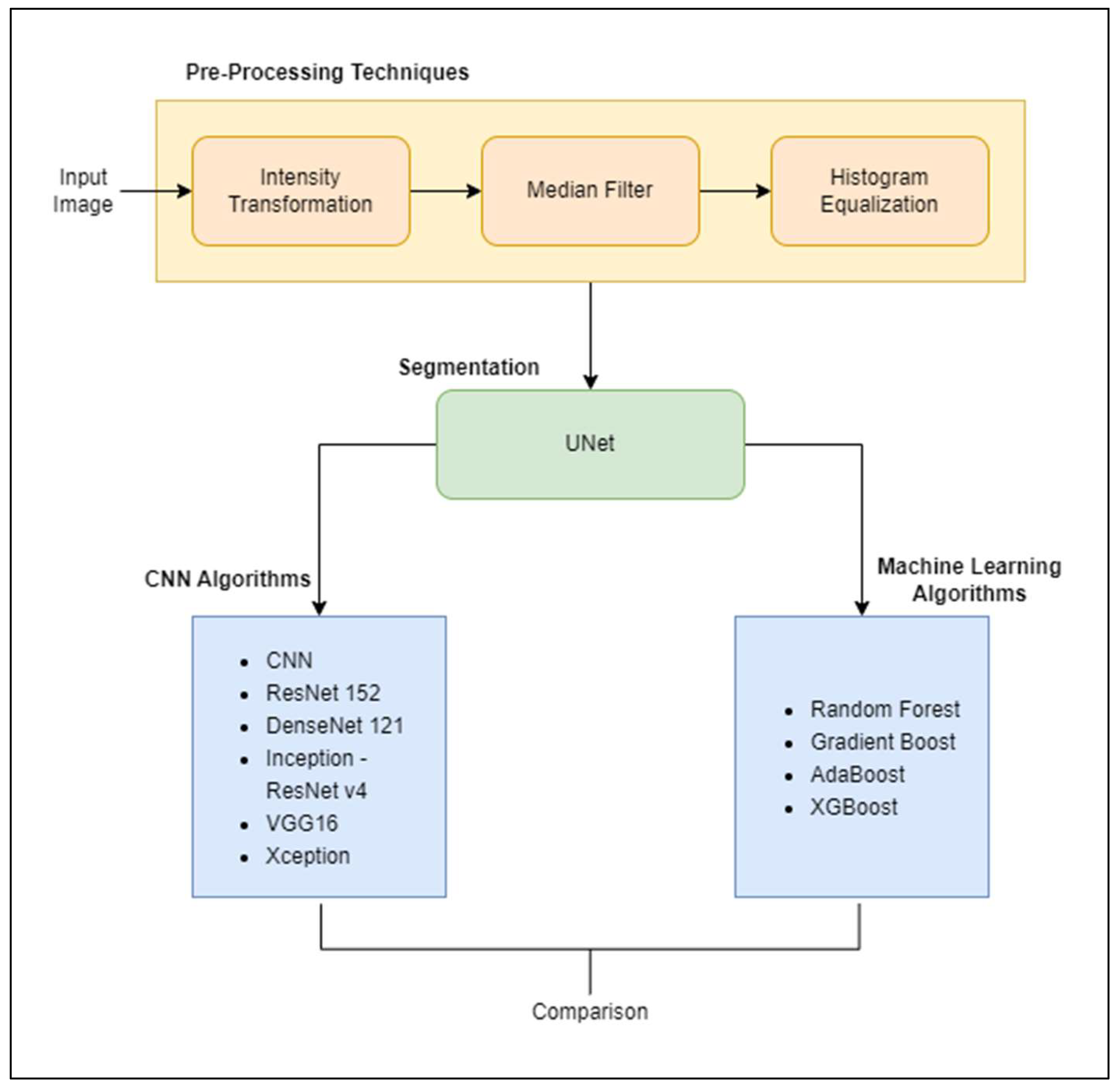
Figure 1 describes the implementation flowchart. The CT scan images, of the ovarian region collected, are used as input images to the algorithms. They undergo Pre-processing techniques before they are fed into these models as input. Pre-processing includes a series of Digital Image Processing techniques to support the segmentation of the input image. Intensity Transformation is performed to obtain higher quality images, by enhancing the pixel intensity in the image. Median Filter is applied to reduce speckle-like patterns formed by noise in the CT scanned image and for better edge detection. Histogram Equalization helps in highlighting fine details in the image to segment out the Region of Interest (ROI), which in our case is the ovarian tumor, with ease.
After undergoing these pre-processing steps, the images are fed as input to a UNet model for segmenting out the tumour in the CT scanned image. UNet [32] is a Convolutional Neural Network (CNN) architecture applied on medical images to perform segmentation tasks. It is mainly used to segment having complex shapes and sizes such as tumors. With its increasing popularity in biomedical imaging, it is also being used in other fields such as satellite imaging etc.
The segmented images are then given as input to several Deep Learning CNN variants and Machine Learning models for classification. The input instances are classified into two categories namely - benign and malignant tumors, to detect whether the subject is at risk of Ovarian cancer or not. The CNN models implemented include simple CNN model, ResNet 152, DenseNet 121, Inception – ResNet v4. VGG16 and Xception. Machine Learning models like Random Forest, Gradient Boost algorithm, AdaBoost and XGBoost are also used. The outcomes of all these algorithms are then compared.

4. Results and Discussions

The result section is divided into three parts. The first section describes the segmentation results using UNet, the second section describes the classification results using variants of CNN and the third section shows the comparison of the deep learning results with Machine Learning results.

4.1. Segmentation Results Using the UNet Model

The performance metrics used to evaluate the segmentation process are Dice and Jaccard score.
Dice score: This metric is used to determine the similarity in two images. Here two images refer to ground truth and the segmented image. The equation for the Dice score is given below:
D i c e = 2 * | S G | S + | G |
where S indicates the segmented region that needs to be evaluated and G indicates the ground truth of the image. |.| indicates the cardinality of the set. Dice score always has a value between 0 and 1. Greater the value, the better is the segmentation.
Jaccard score: This metric is used to calculate the overlap area between segmented and the ground truth. The equation for the Jaccard score is given below:
J a c c a r d = d i c e 2 d i c e
The evaluated values of the Jaccard score range lies between 0 and 1; greater the value, the better the segmentation results obtained.
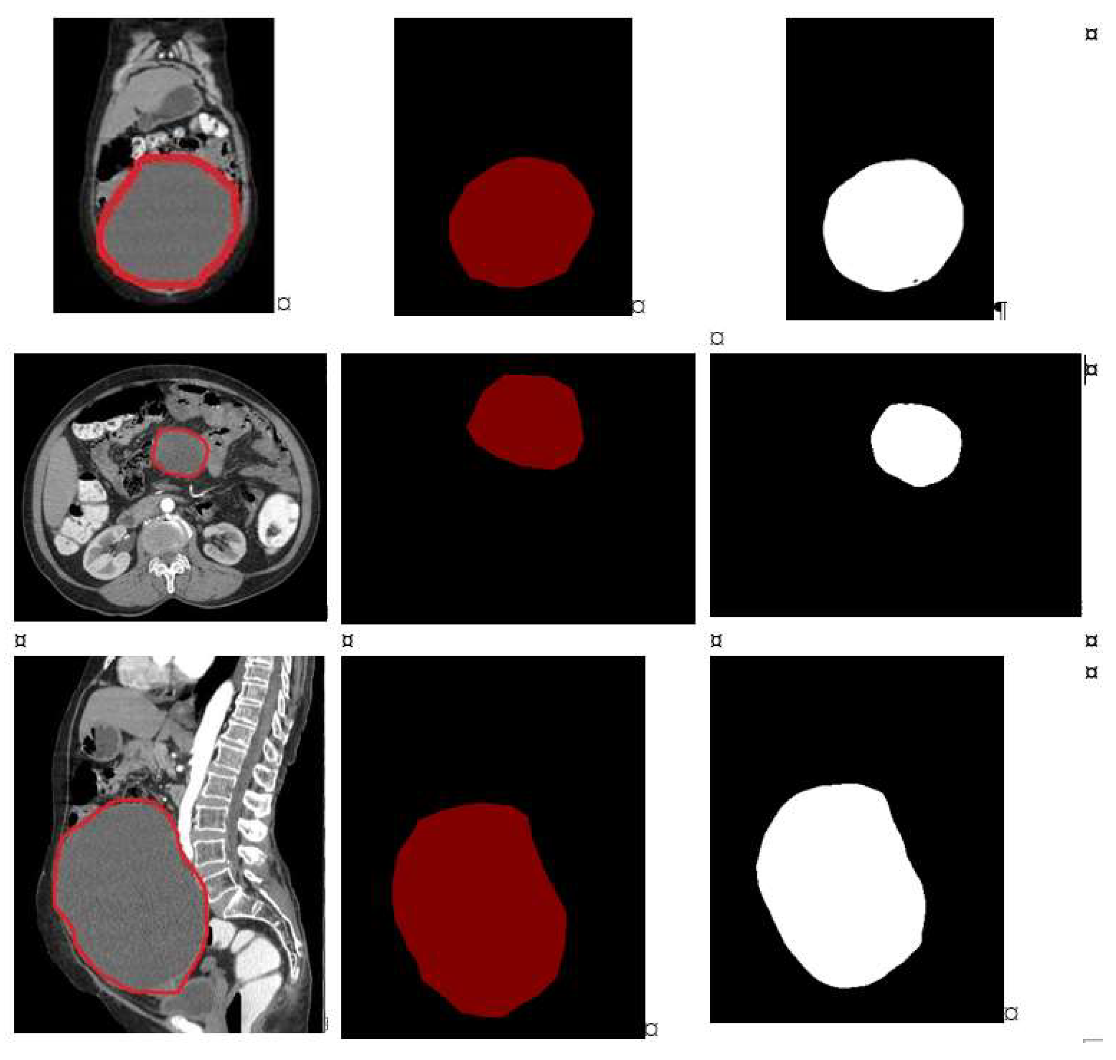
Figure X presents the images of the input, ground truth (label) and the segmented images for benign images. It is observed from Table 1 that UNet performed well for the benign images as the shape of the tumor is well grown and the borders are clear. Table 1 has the 20 sample results from the testing set.
Figure 2. Benign dataset -Towards the left is the input image, middle is the label, and the right is the segmented image.
Preprints 70961 g002
From the Figure 2, it is observed that the ground truth and the segmented images are very close and the same is reflected in the Dice and the Jaccard score tabulated in Table 1. The column “class0” indicates background and the column “class1” indicated the tumor. The average Dice score was 0.998±0.12 for class0, 0.981±0.19 for class1. The average Jaccard score was 0.995±0.22 for class0, 0.964±0.20 for class1.
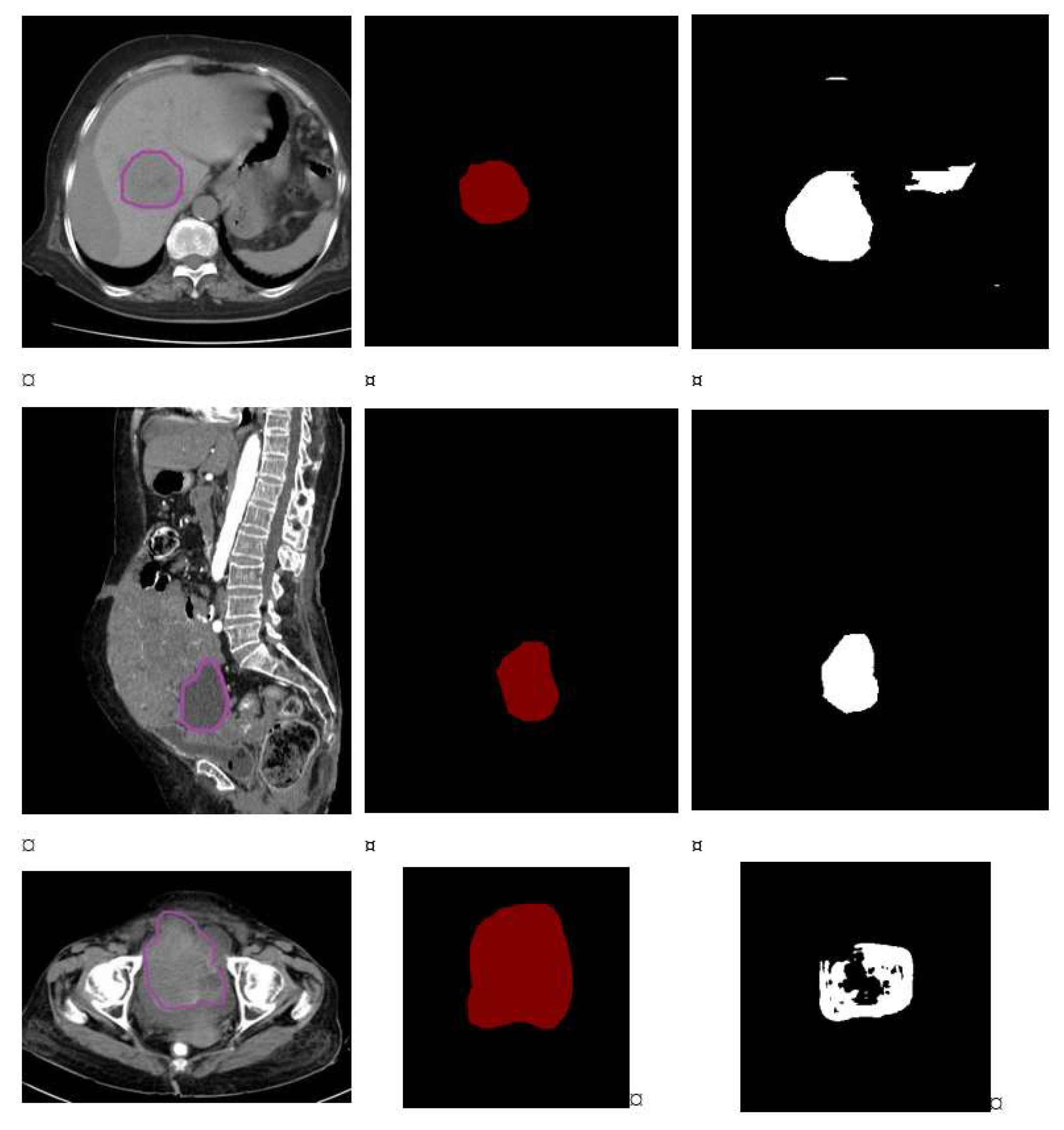
Figure 2 presents the images of the input, ground truth (label) and the segmented version of malignant images. It is observed from Table 2 that UNet did not perform well in detecting malignant instances as the shape of the tumor is very uneven, small and the borders are very uncertain due to the characteristics of the malignant tumors. Table 2 has 20 sample results from the testing set.
Figure 2. Malignant dataset -Towards the left is the input image, middle is the label and the right is the segmented image.
Preprints 70961 g003
From Figure 2, it is observed, from the malignant image in the first row, that the tumor size is very small and that the pixel intensity is very less. Due to size and the intensity, UNet model performance is low with the dice and Jaccard score as follows: class0_dice is 0.98, class1_dice is 0.87 and class0_jaccard is 0.99 and class1_jaccard is 0.84.
On the similar lines, in the malignant image present in the middle row, we observed the tumor has grown fully and the intensity of the pixel is high. Due to this, UNet has performed well with the dice and Jaccard score as follows: class0_dice is 0.996, class1_dice is 0.950 and class0_jaccard is 0.993 and class1_jaccard is 0.926. The malignant image in the last row shares the similar characteristic as the 1st row image. The tumor is very uncertain with respect to size, shape and the border. Hence, lower values are obtained in the segmentation results.
Table 2 shows 20 sample image performance from the test dataset. Due to the nature of malignant tumours’ size, shape, border and intensity of the pixels, the performance of UNet on malignant tumours is overall less when compared to the performance on benign tumors.
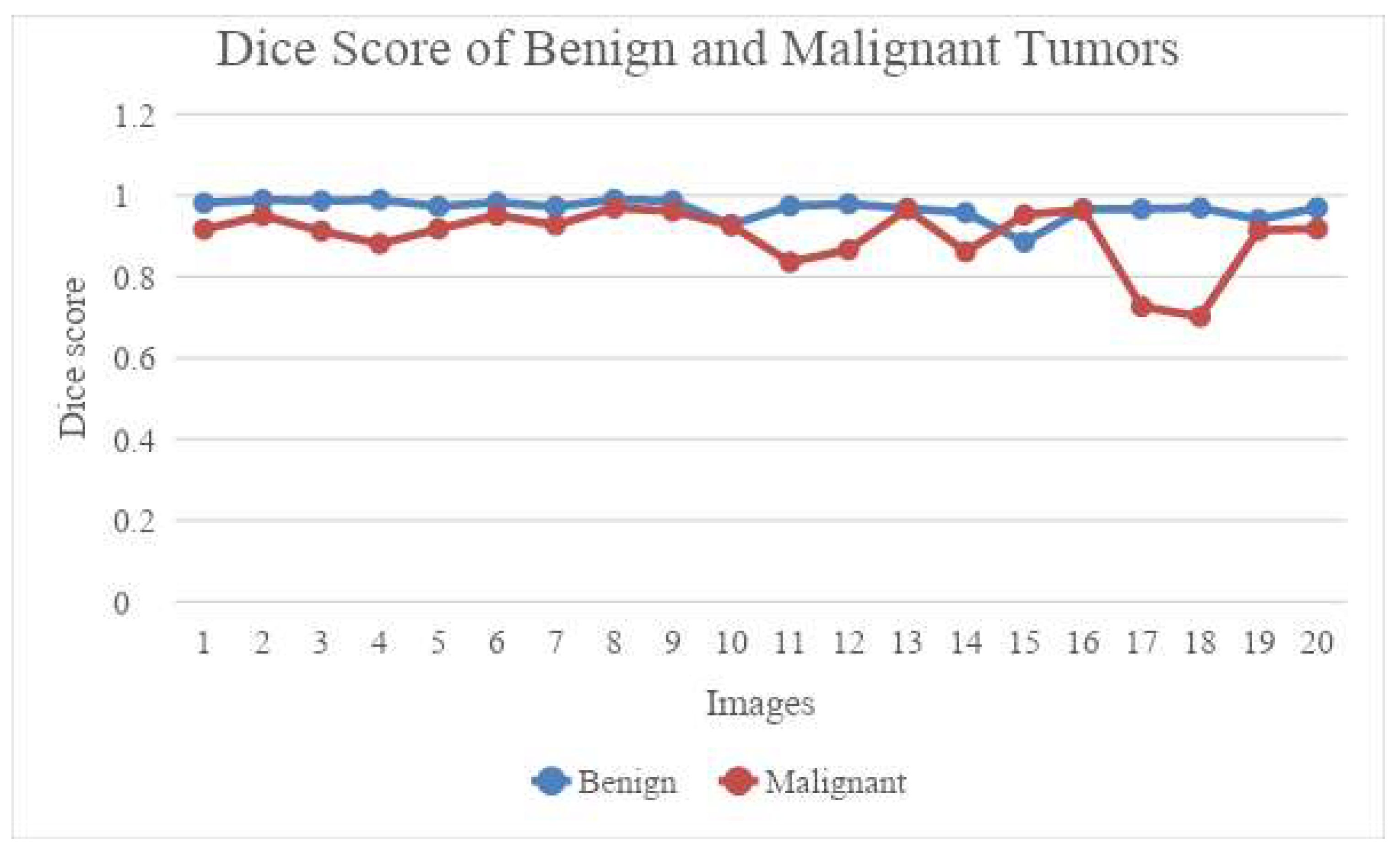
From the graph below, depicted in Figure 3, we see that UNet has performed well on benign images when compared to malignant images. The dice score range for benign images is between 0.992 to 0.998 whereas the dice score for malignant category ranges between 0.70 to 0.91.
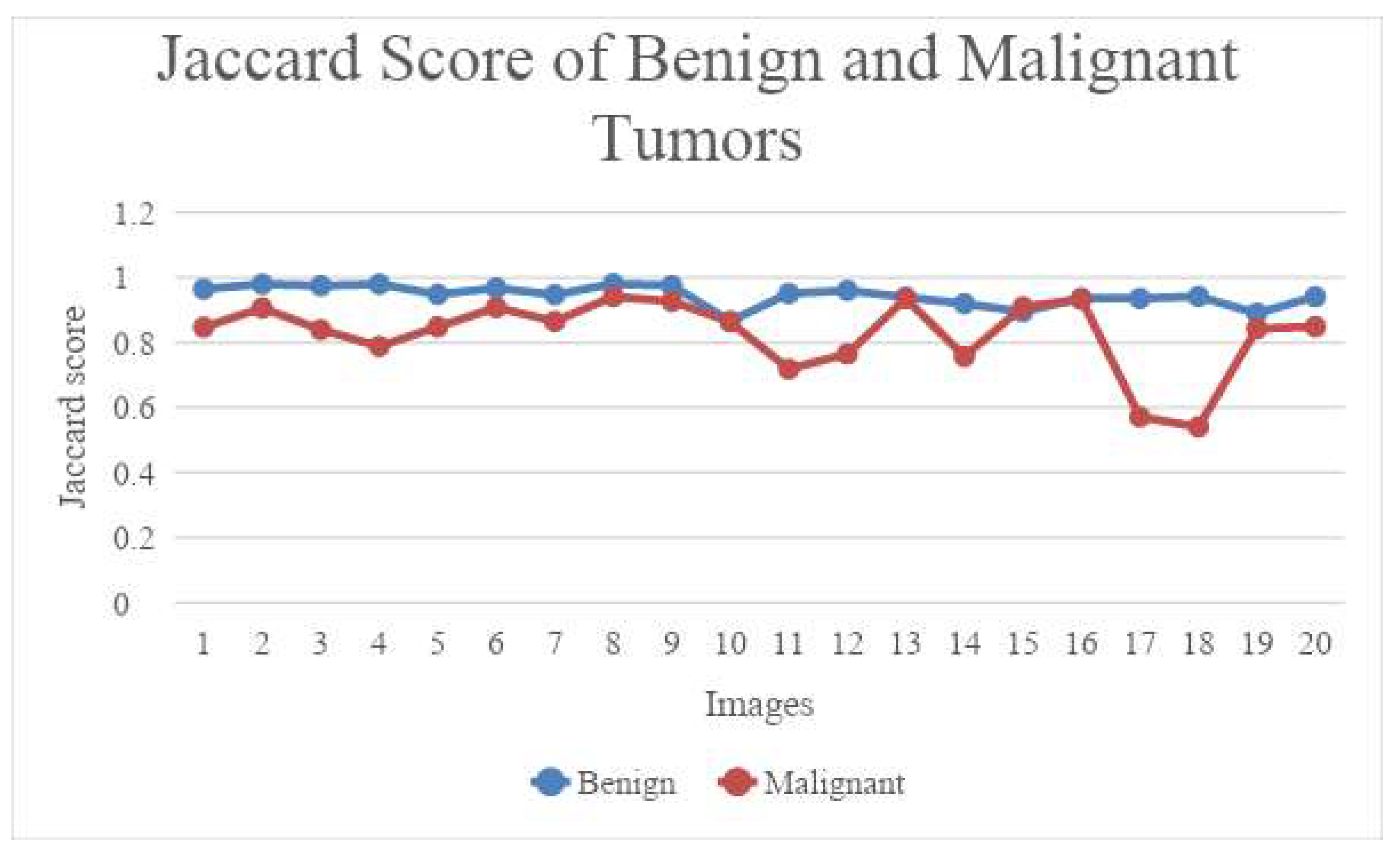
Figure 4 shows the Jaccard score comparison for benign and malignant images.

4.2. Classification Results Using Variants of CNN Model

The different performance metrics used to analyse the classification results in our experiment are: accuracy, precision, recall and F1 score. The metrics are expressed mathematically as follows:
A c c u r a c y = T P + T N T P + T N + F P + F N × 100
P r e c i s i o n = T P T P + F P × 100
R e c a l l = T P T P + F N × 100
F 1 s c o r e = 2 × P r e c i s i o n × R e c a l l P r e c i s i o n + R e c a l l
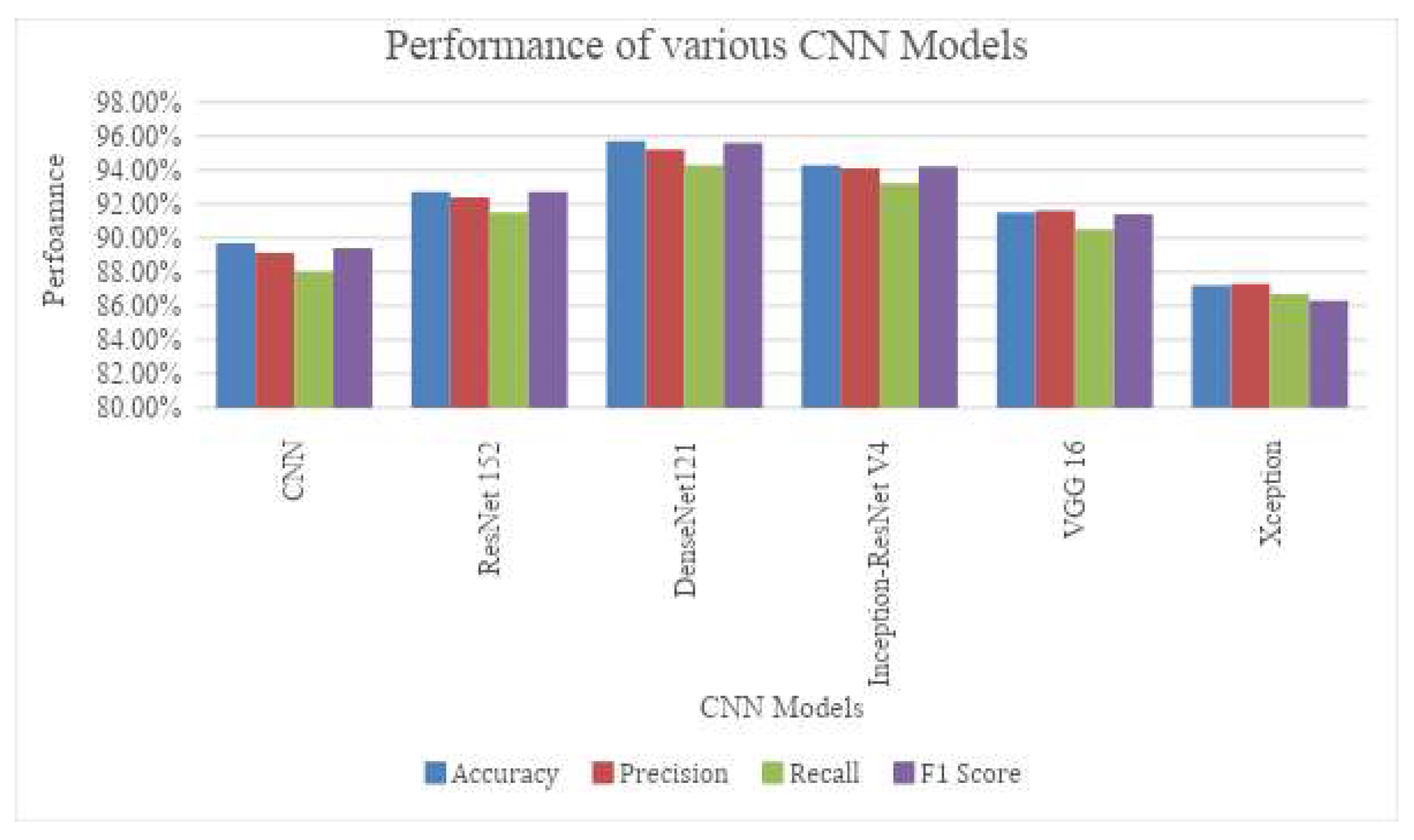
From Table 3 and Figure 5, it is observed that DenseNet121 outperformed the other CNN models used. Owing to the connectivity patterns in the DenseNet architecture, the information will not be lost or vanished by the time it reaches the last layer.
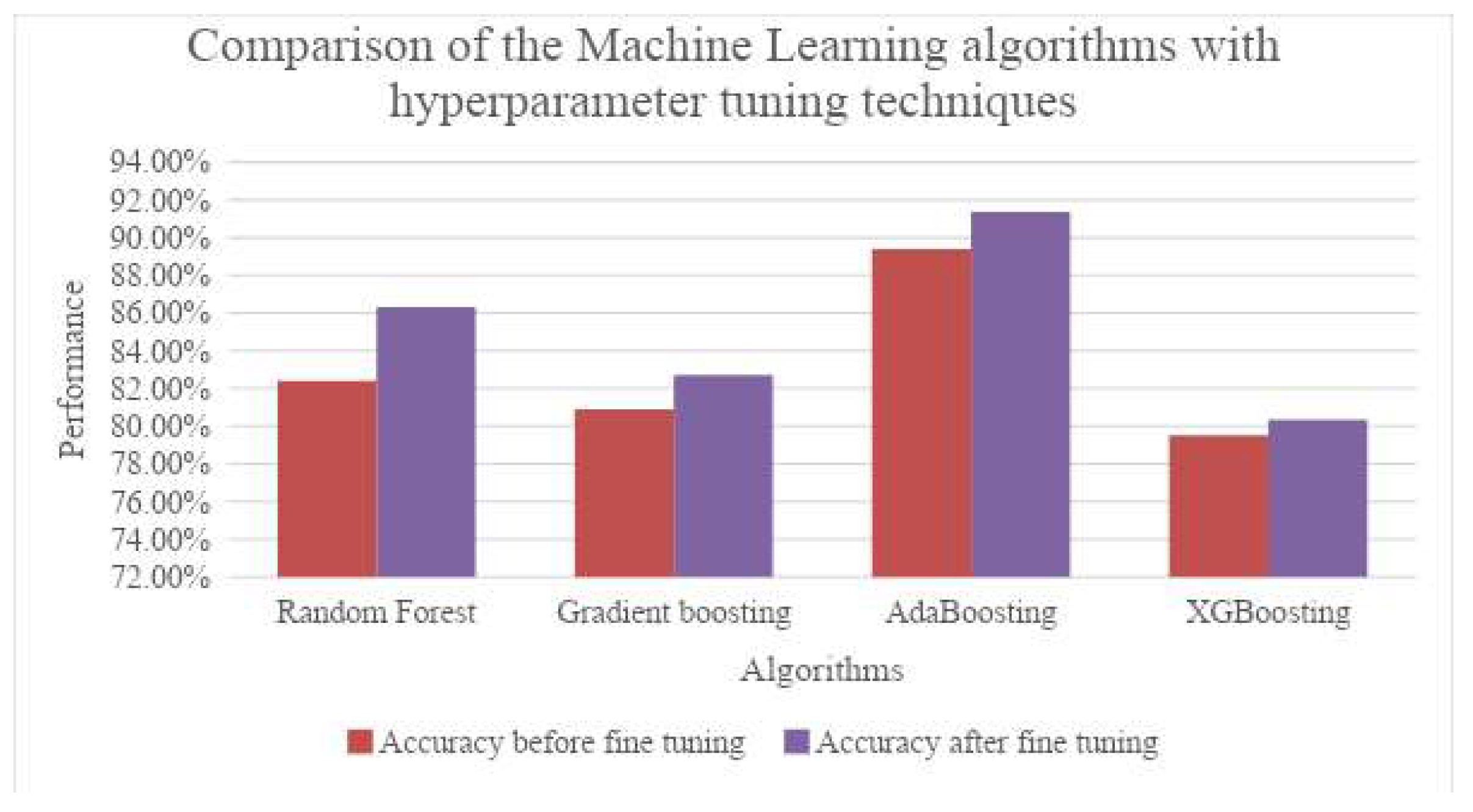
Results are then compared with ensemble machine learning models using the same data, for classification. From Table 4, it can be noted that AdaBoosting outperformed the other ensemble machine learning models. From Table 5 and from Figure 6, it is observed that the performance of the learning algorithms has been improved with the tuning techniques.
The different optimization techniques used for fine tuning the parameters are HyperOpt, Optuna and Multi-Fidelity Optimization After fine tuning the parameters, the improved results using ML algorithms are:

5. Conclusions

Ovarian cancer is one of the most dangerous diseases found in women. An alarming number of deaths are caused every year due to diagnosis of Ovarian cancer only in the third and fourth stages. Advancements in the field of Deep Learning have helped solve several issues in the medical field too. If not as a completely dependable solution, we can find a significant amount of work carried out in helping doctors and radiologists to detect tumors. These computer screening methods take CT scan images of the ovarian region as input and perform pre-processing, Segmentation and Classification on them, using various algorithms. In the current work, multiple algorithms in Machine Learning as well as Deep Learning fields have been implemented and compared. Segmentation is carried out using the UNet model. 20 images are sampled from both the categories – benign and malignant on which the UNet algorithm is applied. The performance is measured using Jaccard score and Dice score. It is found that the model performs better at segmenting benign tumours. The Deep Learning models include several variants of CNNs such as CNN, ResNet 152, DenseNet 121, Inception-ResNet V4, VGG16 and Xception. The evaluation metrics used are accuracy, precision, recall and F1-score. It is observed that DenseNet 121 surpasses the other CNNs in all the metrics while scoring an accuracy of 95.70%. The Machine Learning algorithms involved are Random Forest, Gradient boosting, AdaBoosting and XGBoosting. The same metrics used above are used to evaluate these models as well. Values obtained clearly show that AdaBoosting outperforms the other Machine Learning algorithms considered scoring an accuracy of 89.40% and leading in the other metrics as well. To boost the performance of the Machine Learning models hyperparameter tuning is performed using HyperOpt, Optuna and Multi-Fidelity Optimization techniques. The resulting values were significantly better than sans optimization. However, AdaBoosting still remains the best performing technique amongst the ML models considered. We note that Deep Learning architectures perform more efficiently than Machine Learning models with optimization techniques, in classifying Benign and Malignant Tumors in CT scanned images which proves them to be an aiding tool.

References

  1. Labidi-Galy, S. I., Treilleux, I., Goddard-Leon, S., Combes, J. D., Blay, J. Y., Ray-Coquard, I., & Bendriss-Vermare, N. (2012). Plasmacytoid dendritic cells infiltrating ovarian cancer are associated with poor prognosis. Oncoimmunology, 1(3), 380-382. [CrossRef]
  2. American Cancer Society. (2022). Ovarian Cancer. Retrieved March 28, 2023, from https://www.cancer.org/cancer/ovarian-cancer.html.
  3. Jung, Y., Kim, T., Han, M. R., Kim, S., Kim, G., Lee, S., & Choi, Y. J. (2022). Ovarian tumor diagnosis using deep convolutional neural networks and a denoising convolutional autoencoder. Scientific Reports, 12(1), 17024. [CrossRef]
  4. Wang, X., Li, H., & Zheng, P. (2022). Automatic Detection and Segmentation of Ovarian Cancer Using a Multitask Model in Pelvic CT Images. Oxidative Medicine and Cellular Longevity, 2022. [CrossRef]
  5. Mahmood, F., Borders, D., Chen, R. J., McKay, G. N., Salimian, K. J., Baras, A., & Durr, N. J. (2019). Deep adversarial training for multi-organ nuclei segmentation in histopathology images. IEEE transactions on medical imaging, 39(11), 3257-3267. [CrossRef]
  6. Guan, S., & Loew, M. (2019). Breast cancer detection using synthetic mammograms from generative adversarial networks in convolutional neural networks. Journal of Medical Imaging, 6(3), 031411-031411.
  7. Karimi, D., Dou, H., & Gholipour, A. (2022). Medical image segmentation using transformer networks. IEEE Access, 10, 29322-29332. [CrossRef]
  8. Xu, T., Farahani, H., & Bashashati, A. (2022). Multi-Resolution Vision Transformer for Subtype Classification in Ovarian Cancer Whole-Slide Histopathology Images. [CrossRef]
  9. Li, H., Fang, J., Liu, S., Liang, X., Yang, X., Mai, Z., ... & Ni, D. (2019). Cr-unet: A composite network for ovary and follicle segmentation in ultrasound images. IEEE journal of biomedical and health informatics, 24(4), 974-983. [CrossRef]
  10. Goodfellow, I. J., Pouget-Abadie, J., Mirza, M., Xu, B., Warde-Farley, D., Ozair, S., Courville, A., & Bengio, Y. (2014). Generative Adversarial Networks. arXiv preprint arXiv:1406.2661v1.
  11. Nagarajan, P. H., & Tajunisha, N. (2021). Automatic Classification of Ovarian Cancer Types from CT Images Using Deep Semi-Supervised Generative Learning and Convolutional Neural Network. Rev. d'Intelligence Artif., 35(4), 273-280.
  12. Zhao, Q., Lyu, S., Bai, W., Cai, L., Liu, B., Wu, M., ... & Chen, L. (2022). A Multi-Modality Ovarian Tumor Ultrasound Image Dataset for Unsupervised Cross-Domain Semantic Segmentation. arXiv preprint arXiv:2207.06799.
  13. Saha, D., Mandal, A., & Ghosh, R. MU Net: Ovarian Follicle Segmentation Using Modified U-Net Architecture. [CrossRef]
  14. Jin, J., Zhu, H., Zhang, J., Ai, Y., Zhang, J., Teng, Y., ... & Jin, X. (2021). Multiple U-Net-based automatic segmentations and radiomics feature stability on ultrasound images for patients with ovarian cancer. Frontiers in Oncology, 10, 614201. [CrossRef]
  15. Thangamma, N. G., & Prasanna, D. S. (2018). Analyzing ovarian tumor and cancer cells using image processing algorithms K means & fuzzy C-means. International Journal of Engineering & Technology, 7(2.33), 510-512.
  16. Hema, L. K., Manikandan, R., Alhomrani, M., Pradeep, N., Alamri, A. S., Sharma, S., & Alhassan, M. (2022). Region-Based Segmentation and Classification for Ovarian Cancer Detection Using Convolution Neural Network. Contrast Media & Molecular Imaging, 2022. [CrossRef]
  17. Ahamad, M. M., Aktar, S., Uddin, M. J., Rahman, T., Alyami, S. A., Al-Ashhab, S., ... & Moni, M. A. (2022). Early-Stage Detection of Ovarian Cancer Based on Clinical Data Using Machine Learning Approaches. Journal of Personalized Medicine, 12(8), 1211. [CrossRef]
  18. Kodipalli, A., Guha, S., Dasar, S., & Ismail, T. (2022). An inception-ResNet deep learning approach to classify tumours in the ovary as benign and malignant. Expert Systems, e13215. [CrossRef]
  19. Kodipalli, A., Devi, S., Dasar, S., & Ismail, T. (2022). Segmentation and classification of ovarian cancer based on conditional adversarial image to image translation approach. Expert Systems, e13193. [CrossRef]
  20. Ruchitha, P. J., Sai, R. Y., Kodipalli, A., Martis, R. J., Dasar, S., & Ismail, T. (2022, October). Comparative analysis of active contour random walker and watershed algorithms in segmentation of ovarian cancer. In 2022 International Conference on Distributed Computing, VLSI, Electrical Circuits and Robotics (DISCOVER) (pp. 234-238). IEEE. [CrossRef]
  21. Liaqat, A., Khan, M. A., Shah, J. H., Sharif, M., Yasmin, M., & Fernandes, S. L. (2018). Automated ulcer and bleeding classification from WCE images using multiple features fusion and selection. Journal of Mechanics in Medicine and Biology, 18(04), 1850038. [CrossRef]
  22. Fernandes, S. L., Tanik, U. J., Rajinikanth, V., & Karthik, K. A. (2020). A reliable framework for accurate brain image examination and treatment planning based on early diagnosis support for clinicians. Neural Computing and Applications, 32(20), 15897-15908. [CrossRef]
Figure 1. Flow of the implementation.
Preprints 70961 g001
Figure 3. Dice score comparison between benign and malignant.
Preprints 70961 g004
Figure 4. Jaccard score comparison between benign and malignant.
Preprints 70961 g005
Figure 5. Diagrammatic representation of performance of the CNN models.
Preprints 70961 g006
Figure 6. Diagrammatic representation of the comparison of the results with tuning techniques.
Preprints 70961 g007
Table 1. Dice score and Jaccard score for Benign tumor.
Image Benign
Class0_dice Class1_dice Class0_Jaccard Class1_Jaccard
CT_1 0.99756 0.98193 0.99514 0.96451
CT_2 0.99775 0.98975 0.99552 0.97972
CT_3 0.99758 0.98710 0.99518 0.97454
CT_4 0.99738 0.98974 0.99479 0.97969
CT_5 0.99777 0.97334 0.99556 0.94807
CT_6 0.99701 0.98348 0.99404 0.96751
CT_7 0.99761 0.97269 0.99523 0.94684
CT_8 0.99729 0.99024 0.99459 0.98068
CT_9 0.99895 0.98740 0.99790 0.97512
CT_10 0.99882 0.92817 0.99765 0.86597
CT_11 0.99786 0.97470 0.99577 0.95066
CT_12 0.99814 0.97956 0.99637 0.95994
CT_13 0.99862 0.96864 0.99724 0.93920
CT_14 0.99718 0.95798 0.99439 0.91935
CT_15 0.99460 0.88555 0.98926 0.89461
CT_16 0.99696 0.96709 0.99395 0.93623
CT_17 0.99686 0.96678 0.99375 0.93569
CT_18 0.99777 0.96998 0.99553 0.94171
CT_19 0.99643 0.94171 0.99290 0.88984
CT_20 0.99724 0.96965 0.99450 0.94101
Table 2. Dice score and Jaccard score for Malignant tumor.
Image Malignant
Class0_dice Class1_dice Class0_Jaccard Class1_Jaccard
CT_1 0.99485 0.917209 0.989753 0.847079
CT_2 0.996533 0.950731 0.993091 0.906089
CT_3 0.994843 0.912769 0.989738 0.839535
CT_4 0.996412 0.881644 0.992849 0.788339
CT_5 0.998503 0.9179 0.99701 0.848258
CT_6 0.99661 0.951691 0.993242 0.907835
CT_7 0.997797 0.927598 0.995603 0.864972
CT_8 0.997502 0.969651 0.995017 0.941091
CT_9 0.996653 0.961937 0.993328 0.926665
CT_10 0.995213 0.926677 0.990471 0.863373
CT_11 0.983532 0.836238 0.967598 0.718565
CT_12 0.995118 0.866793 0.990284 0.764902
CT_13 0.999053 0.966729 0.998107 0.9356
CT_14 0.995317 0.861702 0.990677 0.757008
CT_15 0.997093 0.952554 0.994203 0.909406
CT_16 0.997117 0.965229 0.99425 0.932794
CT_17 0.995457 0.727209 0.990954 0.57135
CT_18 0.986163 0.701614 0.972704 0.540374
CT_19 0.998494 0.914519 0.996992 0.842501
CT_20 0.998775 0.918228 0.997552 0.848818
Table 3. Performance of various CNN in classifying the ovarian tumors.
Sl. No CNN Architectures Accuracy Precision Recall F1 Score
1. CNN 89.7% 89.1% 88.0% 89.4%
2. ResNet 152 92.7% 92.4% 91.5% 92.7%
3. DenseNet121 95.7% 95.2% 94.3% 95.6%
4. Inception-ResNet V4 94.3% 94.1% 93.2% 94.2%
5. VGG 16 91.5% 91.6% 90.5% 91.4%
6. Xception 87.2% 87.3% 86.7% 86.3%
Table 4. Performance of Ensemble learning model for classification.
Sl. No CNN Architectures Accuracy Precision Recall F1 Score
1. Random Forest 82.4% 82.7% 83.6% 81.5%
2. Gradient boosting 80.9% 80.3% 80.88% 79.5%
3. AdaBoosting 89.4% 88.5% 89.1% 87.6%
4. XGBoosting 79.5% 80.2% 79.8% 80.3%
Table 5. Improved performance with hyperparameter tuning techniques.
Sl. No CNN Architectures Accuracy Precision Recall F1 Score
1. Random Forest 86.3% 86.3% 87.9% 86.2%
2. Gradient boosting 82.7% 82.7% 83.7% 81.3%
3. AdaBoosting 91.37% 91.87% 90.3% 91.78%
4. XGBoosting 80.34% 81.67% 80.48% 81.78%
Disclaimer/Publisher’s Note: The statements, opinions and data contained in all publications are solely those of the individual author(s) and contributor(s) and not of MDPI and/or the editor(s). MDPI and/or the editor(s) disclaim responsibility for any injury to people or property resulting from any ideas, methods, instructions or products referred to in the content.
Copyright: This open access article is published under a Creative Commons CC BY 4.0 license, which permit the free download, distribution, and reuse, provided that the author and preprint are cited in any reuse.
Prerpints.org logo

Preprints.org is a free preprint server supported by MDPI in Basel, Switzerland.

Subscribe

© 2024 MDPI (Basel, Switzerland) unless otherwise stated