Submitted:
30 July 2024
Posted:
30 July 2024
You are already at the latest version
Abstract
The capacitated lot-sizing problem with product recovery (CLSP-RM) holds significant importance in reverse logistics but is notoriously complex (NP-hard). In this study, two techniques are introduced to confront this challenge. The first technique entails devising a linear optimization task that eliminates capacity limitations across a wide problem spectrum, yielding a remarkably accurate approximation of the optimal solution. This adaptable approach presents a potent alternative and holds potential for extension to diverse problem categories owing to its versatile nature. The second technique employs a simulation methodology utilizing Halton’s uniform random numbers to address the issue. This randomized production search method sidesteps considerations of production costs, inventory expenditures, and production order when determining production batches. The research’s novelty lies in its application of these techniques to the problem. The suggested methods undergo evaluation via a benchmark dataset of approximately 4200 instances, with comparison against solutions derived through the Gurobi solver. The results underscore the efficacy and resilience of the introduced methodology in tackling the CLSP-RM predicament.
Keywords:
simulation based optimization
; capacitated lot-sizing problem
; heuristics
; remanufacturing
1. Introduction
Two seminal papers have profoundly shaped the landscape of the Lot Sizing Problem (LSP). The inaugural paper, known as the Dynamic Economic Lot Sizing model (DLS), was concurrently introduced by [1,2], and is widely recognized as the Manne-Wagner-Whitin Model. In its "classical" rendition, the DLS addresses a discrete-time, finite-horizon inventory management challenge involving a singular item. Its primary objective is to efficiently meet deterministic time-varying demands through optimal stock management or procurement strategies, with further elucidation provided in ([3]). The second pivotal paper, the Economic Lot Scheduling Problem (ELSP), was brought forth by Elmaghraby ([4]). Both of these works tackle a fundamental issue within production planning determining optimal lot sizes and production schedules for a multitude of items produced on a shared production line or machine. The overarching goal is to minimize expenses associated with production and inventory while simultaneously fulfilling demand requirements and adhering to pertinent production constraints. Supplementary insights can be found in ([4]). Researchers have further expanded upon the work of Elmaghraby and Manne-Wagner-Whitin to tackle variations and more advanced versions of the ELSP and DLS. These advancements include incorporating uncertainties, time windows, and remanufacturing into the models. For a comprehensive overview of the economic lot sizing problem, readers can consult [5,6]. The Economic Lot Scheduling Problem (ELSP) with remanufacturing options (ELSPR) represents an extension of the classical Wagner Whitin model. A notable enhancement is the incorporation of a distinct element: within each time period, predetermined quantities of used products are introduced into the system. These returned items offer the potential for remanufacturing, serving to fulfill demand alongside the conventional manufacturing processes. In recent decades, there has been a growing emphasis on production planning, particularly with regard to incorporating recycling options [7]. The literature outlines two distinct categories of recycling production planning problems.
In the first category (Cat. 1), the primary objective is to meet the external demand for products through either remanufactured or newly produced goods Figure 1. This category focuses on regulating two types of inventories: the inventory of new products and the inventory of remanufactured products. It is assumed that both new and remanufactured products are identical and, thus, considered serviceable entities that can fulfill demands. Numerous authors have extensively studied this category [8]. This category also encompasses issues related to pricing and lot sizing, wherein demand is fulfilled through various substitution alternatives.
The second category (Cat. 2) deals with two distinct demands: one for new products and the other for recycled products. Additionally, this category introduces a key feature where a deterministic quantity of returned goods enters the system in each period. These returned items can be remanufactured and used to meet the demand for remanufactured products, complementing the regular production of new items. As a result, the inventory includes three types of stocks: new products, remanufactured products, and returned products Figure 1.
In specific industrial sectors, such as the paper industry, two different types of demand are observed: one for recycled paper and the other for paper made from new fiber. Recycled paper is typically priced lower due to its reduced water and energy consumption during production, compared to virgin fiber papers [9]. Moreover, recycled paper often benefits from shorter transportation distances as it is sourced locally, while virgin fiber and new fiber papers are imported from other countries in larger quantities. This observation extends to other sectors, including photocopiers, tires, and personal computers see [10,11].
Publications regarding Category 1: Building upon Elmaghraby’s groundwork (see [4]), Tang and Teunter ([12]) investigated the hybrid production line’s multi-product dynamic lot sizing. This involved manufacturing new products and remanufacturing returns, with a single manufacturing and remanufacturing lot per product synchronized within a common cycle. They constructed a Mixed Integer Linear Programming (MILP) problem for precise resolution. The multi-product dynamic lot sizing problem with distinct manufacturing and remanufacturing sources, each operating on separate dedicated lines, was further examined in [13].
In a study by [14], a multi-item economic lot-sizing problem involving remanufacturing and capacitated production was examined. The study drew upon the concept introduced by Garfinkel and Nemhauser (1969), known as the Set Partitioning Problem (SPP). Another contribution, by [15], delved into the multi-item economic lot-sizing problem with remanufacturing and uncapacitated production. They extended the model initially proposed by [16] and put forward two innovative variations of the Variable Neighborhood Search (VNS) algorithm. These variants aimed at discovering optimal solutions for the ELSR problem. In a separate work, [17] introduced an effective Mixed Integer Programming (MIP)-based matheuristic for the multi-item capacitated lot-sizing problem with remanufacturing (CLSP-RM). Notably, this approach addresses capacity constraints individually for new and remanufactured products.
[18] conducted a comparative analysis of MIP approaches for the economic problem of single-item lot-sizing with remanufacturing (ELSR) and uncapacitated production. They proposed a shortest path formulation. [19] contributed a polynomial-time heuristic within this category. Their work also includes a comprehensive compilation of methods developed by [20,21,22,23,24]. Addressing an extension of the economic problem of single-item lot sizing, [25] introduced considerations for remanufacturing, final disposal, and distinct demand flows for new and remanufactured products. This extension also accounted for a unidirectional substitution, wherein the demand for remanufactured products can be satisfied by new items, but not vice versa. The authors proposed both a network flow formulation and a pseudopolynomial time dynamic programming algorithm. Notably, the model does not incorporate capacity constraints.
Publications regarding category 2: By [26] address the production planning problem within a hybrid manufacturing and remanufacturing system (HMRS). They postulate a multi-objective mathematical model (MIP) whose objective is to determine a production plan taking into account the available capacities in each period, which satisfies the demand for new and remanufactured products and minimizes all costs of production, storage and disposal of new products, as well as the minimization of CO2 emissions generated in production. They introduce a solution method based on a non-dominant sorting algorithm (NSGA-II).
[27] investigates the joint problem of pricing and lot sizing in a hybrid manufacturing and remanufacturing system with a one-way substitution option. Two demand performances, for new and remanufactured items, are considered in this paper. In the case of a shortage of remanufactured items, a one-way substitution option is assumed, so that the demand for these remanufactured items is satisfied with new items. The presented mathematical model is an MIP but without capacity constraints. As a solution method they adapt "the cost and benefit heuristic" (CB-heuristic) introduced by [28] and also a memetic algorithm which is improved with the help of a local search.
Zhang et al. ([29]) investigate the capacitated lot sizing problem in closed-loop suply chain considering setup costs, product returns, and remanufacturing. They present a Lagrange relaxation to solve the problem. Based on Zhang’s model we formulate the same problem but taking more general capacity constraints and doing more extensive numerical experiments.
The capacitated lot-sizing problem model is NP-hard. The proof of this statement is to be found in [30,31]. [32] has shown that even the two-item problem with constant capacity is NP-hard. Heuristic methods employed for solving problems within the CLSP class typically rely on a wide range of sorting rules and other criteria derived from factors such as demand, capacity, setup costs, inventory costs, and production costs. Examples of such heuristic methods include those presented in references like [22,23,33,34]. The achieved solution margin tends to vary within the range of 1% to 10%, as reported in references such as [29,34].
1.1. Research Contributions
This study incorporates two significant constraints. The first constraint ensures that the cumulative demand for both new and remanufactured products remains within the cumulative capacity for each period. The second constraint mandates that the cumulative demand for remanufactured products during each period does not surpass the cumulative quantities of used products returned within the same period. No specific relationship is imposed between the existing capacities and the quantities of returned products. This particular characteristic, which is overlooked in certain promoted publications, adds an additional layer of complexity to the problem, rendering it non-standard in nature.
The contribution of this work can be summarized as follows: We examine two overarching problem classes under the framework of the aforementioned capacity constraints. These classes are as follows:
- The first class involves production periods where the demand for both new and remanufactured product exceeds the available capacity within those specific time frames. To address this scenario, we propose a linear program devoid of capacity constraints, providing a highly accurate approximation of the optimal solution.
- In the second problem class, each period experiences demand that falls short of the existing capacity. This specific problem category exhibits an NP-hard nature, leading us to adopt a direct simulation approach. Additionally, the quasi-random numbers , introduced by [35,36,37], showcase significant properties, as evidenced by [38]. Among these characteristics, their uniform distribution stands out. Accordingly, we present a straightforward simulation utilizing these quasi-random numbers (). Irrespective of the input parameters, we organize production based on both feasibility and randomness. Starting from the initial production period, we define lower and upper limits for viable production ranges of the new product. This production information informs the establishment of production range limits for the remanufactured product. The order in which the new or remanufactured product is produced holds no significance in the algorithm’s execution. These defined limits delineate production intervals that strictly adhere to all problem constraints. Within each interval, a random production quantity is generated using uniform random numbers derived from the Halton sequence. It is imperative to emphasize that the random production process significantly influences the subsequent determination of feasible production intervals.
- Moreover, our heuristic approach ensures the generation of a feasible solution whenever the problem is solvable. After simulating N production plans, we select the most cost-effective one. This solution is then compared against numerical solutions obtained through the Gurobi solver. The scheduling process is straightforward, and the results prove to be quite satisfactory given the scale of the presented problems.
1.2. Outline
The rest of the paper is organized as follows: Section 2 we propose a new mathematical programming formulation for the problem. In Section 3 we present a relaxation of the problem without capacity constraints (Model A) and we will see that the solution obtained for the chosen class of tasks is very close to the optimal solution of the original problem. In Section 4, we present a heuristic solution method (Model B) for another class of tasks. In Section 5, we report the results of computational experiments. In Section 6 we present some conclusions and suggested directions for further research.
2. Problem Description
We assume that a factory produces two types of products, one manufactured from raw materials and the other remanufactured from collected used products. The demands for these two products are separate, deterministic, and time varying during a finite planing horizon, and should be satisfied without backlogging. The costs consist of fixed setup cost, linear production cost proportional to the production quantity, and linear inventory holding costs. All cost components are considered for both manufacturing and remanufacturing activities per unit and periode [29]. The following Table 1 summarize the notation used in this paper.
We make the following assumptions
- The demand for new products and remanufactured products are separate and backlog is not allowed.
- The manufacturing capacity is sufficient to meet the demands in each period, in particularly we have: the capacity can satisfy the demands for new products and remanufactured products simultaneously, i.e.
-
Initial and end inventory stocks are zero, 1 i.e.The demand will be fully satisfied if the final inventories are zero.
- The quantity of returned products can satisfy the demand for remanufactured products i.e.
-
In economic terms, inventory holding cost of returned products is less than that of remanufactured products.This hypothesis can be found in [39] too.
Hence, the problem can be formulated as
subject to
The objective function (5) minimizes the sum of setup cost, production cost, and inventory cost for new products and remanufactured products in all periods. Constraints (6),(7) and (8) are the inventory balance constraints for new products, remanufactured products and returned products. Constraints (9) represent capacity constraints for manufacturing and remanufacturing activities. Constraints (10), (11) allow production only with the according setups (i.e ) (12) and (13) are the standard integrality and non-negative constraints.
2.1. Rewriting the Optimization Problem
are replaced in the objective function by
And with a bit of algebraic transformations, we obtain
With the notation
our model is finally
Subject to
3. Model A (Relaxation)
According to our conditions(1) and (3) the general problem has a solution, if the total pro-period demand is less than the pro-period capacity (i.e.). However there are situations, where conditions (1) and (3) are satisfied but is not satisfied e.g. Table 3. We need a feasibility routine which ensures that all demand is satisfied without backlogging. Indeed there are periods (or could be) in which total demand exceeds total capacity. In this case some inventory will have to be build up in earlier periods which slack capacity. We explain how to shift excess demand to earlier periods in which slack capacity is available. We use and complement the idea of [40].
We define
It is easy to see that the sum is null.
Remark 1.
The vector is very useful. Because gives the amount of stock to accumulate () or reduce () in each period so that production does not exceed available capacity pro period. And allows us to determine a good permissible solution.
We see that the demand transformation done in Table 4 is a valid (permissible) solution to the problem (16)-(24). There are many ways to make this transformation, and for this reason to transform the demand in an optimal way we formulate the following problem.
Subject to
If the model (25)-(33) has no solution, it means the model (16)-(24) has no solution too.
We have a problem with no capacity restrictions. We solve this problem and compare it with the optimal solution of the initial problem (16)-(24).
Remark 2.
4. Model B (Simulation)
4.1. Low Discrepancy Sequences
The generation of random numbers with a computer is not possible Knuth [41]. As John von Neumann said: Any one who considers arithmetical methods of producing random digits is, of course, in a state of sin, [42]. An excellent overview of the methods of generating pseudo-random numbers are available [e.g. [41,43,44].
In this section we explain the number-theoretical concept of discrepancy. Then, we introduce the Halton sequence which is probably the easiest low-discrepancy 2 number generation method to describe.
Definition 1.
Let a sequence of real numbers with . The discrepancy for the sequence is defined as
where l is any subinterval and denotes the number of elements of the sequence, that belongs to the interval
A measure for how a sequence of real numbers , is equidistributed on an interval is the discrepancy . Low-discrepancy sequences, also known asquasirandomsequences, are numbers that are better equidistributed in a given volume than pseudo-random numbers.
Remark 3.
A sequence of real numbers is said equidistributed on the interval if [35].
The ( ) of Halton, Sobol and Niederreiter have a low discrepancy . While pseudorandon sequences have a discrepancy [45]. Figure 2 uses two-dimensional projection of a pseudorandom sequence and of a low-discrepancy (Halton) sequence to demonstrate the fundamental difference between the two classes of sequences.
The desirable properties of a sequence of this ( ) may be summarized as follows see [37]:
- the least period length should be sufficiently large,
- it should have littie intrinsic structure (such as lattice structure),
- it should have good statistical properties,
- the algorithm generating the sequence should be reasonably efficient.
It’s easy to generate sequences of Halton with the following Algorithm 1.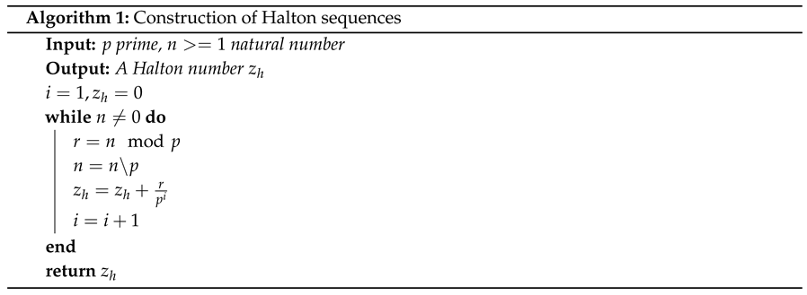
The following Halton sequences of Table 5 are constructed according to Algorithm 1 that uses a prime number as its base.
Remark 4.
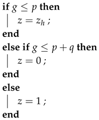
To generate the n-th Halton point in a sequence consider the base ary expansion of a where the ary coefficients Then the n-th Halton point is It’s easy to build a Halton-sequence with the following observation: If then else if then where (details see [38]). This method is very efficient and will be used in this paper.
4.2. Notation
We use the following notation
| Name | Meaning | ||
| = | = | 0 | |
| = | = | 0 | |
| = | = | 0 | |
| = | = | 0 | |
| = | = | 0 |
The notation means and the number z is simulated with the following distribution
We generate a pseudorandom number to decide, that values take z, see Algorithm 2.
4.3. Simulation
The simulation is based on the following lemma.
Lemma 1.
Let and Then
Proof.
The proof proceeds by induction on t. In fact, if because and , we can choose such that .
By induction hypothesis
Then we can choose such that □
Remark 5.
If in Lemma 1 then production in period t is because production up to period satisfies demand up to period t.
Remark 6.
Lemma 1 gives the following lower bound for the production of the products
4.4. Basis of the Simulation
The production plan is created step by step starting from period . To determine the production in period t, we know the selected production until period . In each period, using the constraints of the task (16)-(24) for the production of the products, we determine a lower and an upper bound. Then the production quantity is chosen randomly between the lower and upper limits. These production quantities affect the lower and upper bounds of the future period. We continue in this way until the period . Then we calculate the value of the cost function(i.e., objective function). We repeat this procedure (N times) and choose the production plan with the lowest cost. The advantages of this method is that we do not have to worry about the inventory, production or setup costs. The method is now presented in more detail.
Proposition 1.
If then else
Proof.
From (17) we get
If then total production of new products up to period satisfies total demand up to period t and therefore nothing is produced in period i.e. .
If then the production has a lower bound. From (40) we obtain
□
Proposition 2.
If then else and
Proof.
From (18) and (19)
If , then total production up to period satisfies total demand up to period t and therefore nothing is produced in period i.e. .
If then the production has an upper and lower bound. From (43) results the assertion. □
Proposition 3.
If and then
And
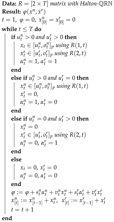
4.5. Simulation of the Objective Function
Let R be a matrix with Halton’s
We simulate the production starting in period t=1. The calculation of the objective function is carried out with Algorithm 3 using proposition 1, 2 and 3.
| Algorithm 3:Calculation of the objective function |
 |
Further information on the complexity-theoretic approach to randomness can be found in [45,46] and [47].
Remark 7.
- The generation of the matrix requires operations.
- Die evaluation of the function with Algorithm 3 requires operations
Then, the computational complexity of the simulation with N points and T periods is
5. Numerical Experiments
5.1. Test Design
We analyse the quality of our solution approach of model A and model B by defining 11 problem classes (PC) by varying the number of periods, see Table 6. The planning horizon T is made very large because in the paper industry planning is done daily. Each PC consists of 200 test instances (TI). In model A, 1824 of the 2200 TI were solvable, in model B 2200. In total, we examined 4024 TI 3+. Model A and Model B are implemented on a computer with , ,.
We vary different parameters to define the TI, e.g., the time between orders (TBO) to determine setup costs. The specifications of the parameters are designed in an exaggerated form, which may not occur in practice, to make the TI as difficult as possible.
The parameters for generating data sets (see Table 7) use the following notation where is a random number, that means the values are uniformly distributed on the interval
5.2. Model A
We randomly generate capacities , then with condition (1) randomly generate aggregate demand . This latter is then randomly cut into and . The remaining parameters according to Table 7.
5.2.1. Results of Model A
The solution of problem (25)-(33) (TD) and the optimal solution of problem (16)-(24) (OP) were found with the Gurobi solver version 9.0.3.
We randomly generated 200 instances per PC and usually between 10 and approx. 20% of the instances have no solution (see line Count). This justifies the fact that the problem is not standard. For example, in Table A1 we see that of the 200 instances for problem class , only 167 had a solution.
With the following notation, we can better understand the results of Table A1.
| T | |
| m | |
| solution of problem (25)-(33) | |
| solution of problem (16-(24) | |
In Table A1 the relative error for Total costs (Tc) and CPU-time for every problem class was calculated as
This is exactly how we calculated the relative errors in inventory cost and setup cost.
Attached in Appendix A are the results of the average total cost, average CPU time, average Inventory costs
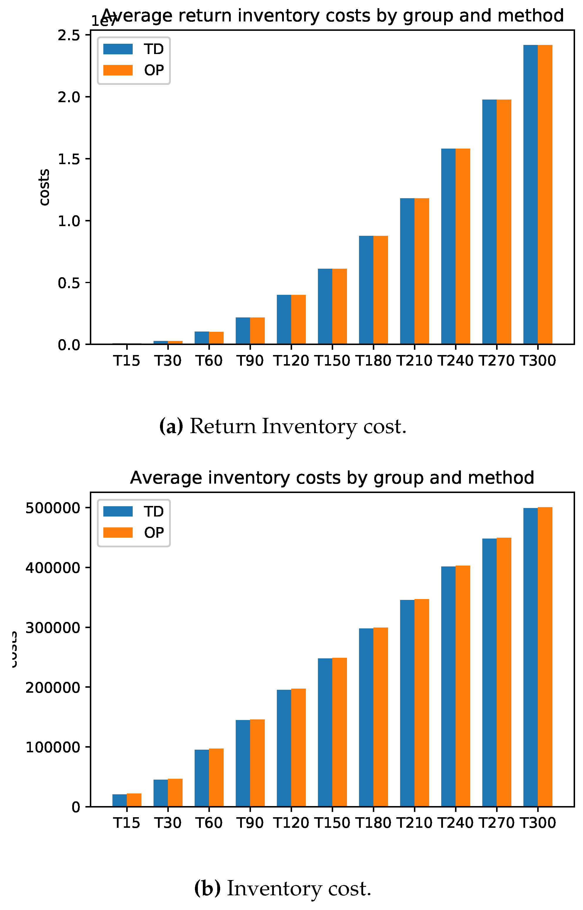
There is hardly any difference between the cost of relaxation (TD) and the original task (OP). Only the computation time for relaxation is faster. The longer the planning horizon, the smaller the difference between the optimal solutions of the problems TD and original optimization task OP. This feature applies to the stocks of the return and setup costs too. On the other hand, the inventory costs for problem TD are always smaller than the inventory costs of problems OP. For more details, please see Figure A1 and Appendix A.1 for the exact calculations. However, we see beyond doubt that this class of problems can be solved very well either with the relaxation TD or directly with a standard solver (here Gurobi).
5.3. Model B
[30] have shown that several families of CLSP are NP-hard. For the construction of the NP-hard instances (2200 instances) we follow the findings of [31]. They use the following notation , where and σ specify respectively the number of items, a special structure for the setup costs, the holding costs, production costs, and capacities. In this paper [31] show that the following class 2/C/G/A/C is NP-hard. For this reason we have created 2200 instances, where the set-up costs per product and capacities per instance are constant. The holding costs do not necessarily follow a specified pattern, the production costs can be chosen arbitrarily. The maximum calculation time for Gurobi is 600 seconds. The heuristic operates according to the number of simulations, which gradually increases with the number of periods. The largest group T300 uses 130 seconds. The parameters for generating data sets (see Table 8) use the following notation where is a random number, that means the values are uniformly distributed on the interval
The important assumption in model B is: the capacities for each TI is constant, the set-up costs in each TI and for each product are constant. These parameters vary between a minimum and a maximum depending on the T parameter.
The capacities for each TI vary according to the parameter T. For example if the capacities are between 600 and 800. If the capacities vary between 3000 and 5500. Analogously the other parameters. The remaining parameters according to Table 8.
For the simulation we used following parameters:
is the Halton’s numbers used for periods.
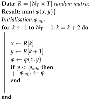
All instances for have the same schema Step 1 until Step 5. We used (see Table 9).
| Algorithm 4:Heuristic: blind search |
 |
5.3.1. Results of Model B
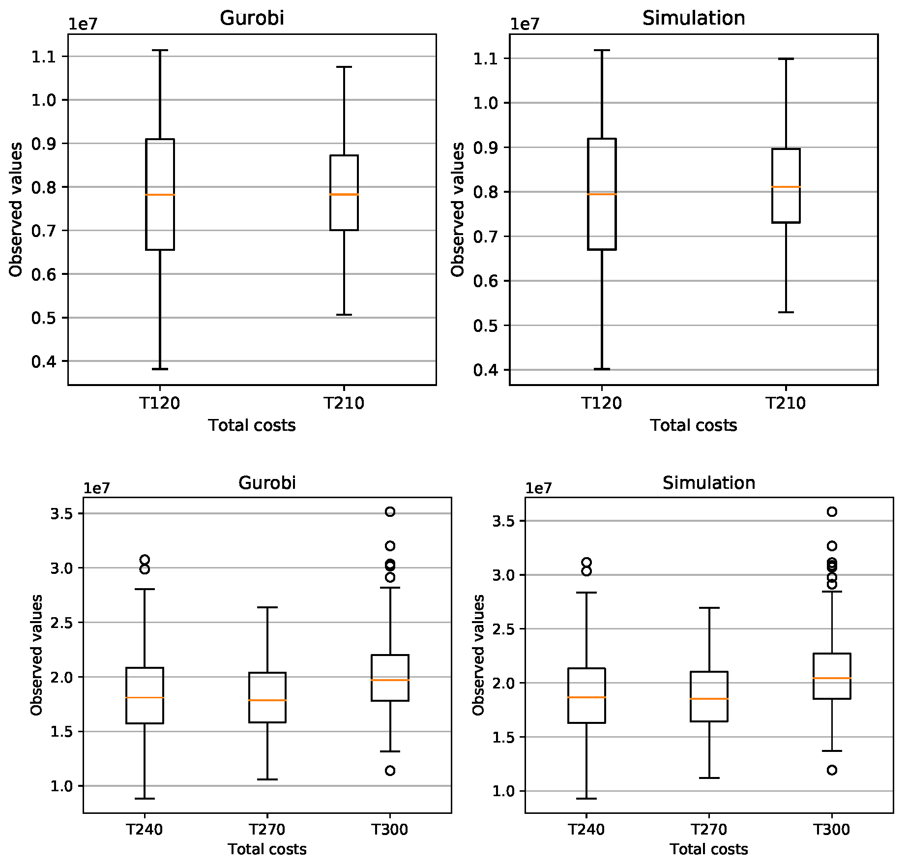
We generated 200 random instances for each problem class (PC) and with a Box-plot we compared the feasible solutions of the problem (16)-(24 ) found by Gurobi 9.0.3 with the solution of the simulation presented in this paper and clearly see the similarity of the results found (see Figure A4 and Figure A5).
With the following notation we present the results (see Table A3).
| T | |
| m | |
| with Simulation | |
| with Gurobi |
In Table A3 the relative error for Total costs (Tc) and CPU-time for every problem class was calculated as
The graphical comparison is shown in Figure A3.
This is exactly how we calculated the relative errors in inventory cost and setup cost. Attached in Appendix B are the results of the average total cost, average CPU time, average Inventory costs. Figure A3 (average CPU time) clearly shows that the Gurobi admissible solution for the PC from T150 to T300 are not optimal and that the CPU of the simulation is much faster.
The simulation in average determines the setup costs and return inventory costs always higher than Gurobi. On the other hand, the inventory costs of Gurobi are higher than the simulation. What can we say about the quality of the solution of the problems? The simulation could not give a better solution than Gurobi’s solution. Gurobi solved the (PC) problems up to T120 in an optimal way. The problems from T150 to T300 were not solved optimally by Gurobi, since it would take too much time due to the NP-hard category of the problem. The simulation found feasible solutions much faster than Gurobi. Here is the advantage of the simulation, the simplicity of its implementation and the speed in finding an acceptable solution.
6. Conclusions and Outlook
We have analyzed a problem that belongs to the NP-hard class. However, the choice of the parameters is very important to obtain a problem that is really NP-hard. With the choice of parameters made in model A, we see that this class of problems is easily solved with a standard solver. By doing a relaxation of the problem, the solution is found more quickly. The error rate is between 0.02% and 2% (taking into account more than 1800 instances). In addressing more intricate CLSP class problems characterized by Model A, the solution derived from Model A can serve as an initial approximation for tackling the problem. This initial approximation can then be seamlessly integrated into various heuristic or metaheuristic approaches.
If we choose the parameters according to model B, Gurobi needs a lot of time to find the optimal solution. In this kind of problem, the presented simulation can help a lot in finding a good solution. We have seen that the error rate is between 1.7% and 3.5% (taking into account more than 2000 instances). On average Gurobi solves the problem with a maximum time of 600 seconds better than the simulation. The great advantage of the simulation is that the calculation is extremely fast and easy.Thanks to the Halton numbers, few simulations are needed to obtain a very good approximation of the solution.
The quality of the solutions can be improved by increasing the number of simulations but it is necessary to have a fairly fast computer. In this work we use at most 10 million simulations. Another parameter that influences the quality of the solutions is the correct choice of the probability p (see (35)). Is there an optimal probability? This is a question for further research.
The simulation possesses a broad nature and can be tailored to examine additional, intricate production issues within the NP-hard category. The benefit is readily apparent: it circumvents the necessity for an extensive array of sorting rules and additional criteria stemming from factors like demand, setup expenses, production outlays, or capacities.
Acknowledgments
I extend my heartfelt gratitude to Robert W. Grubbström and Chistian Almeder for their invaluable insights and thoughtful comments on this paper.
Appendix A. Results Visualization
Appendix A.1. Model A
Figure A1.
Model A: Average Total cost and CPU Time.
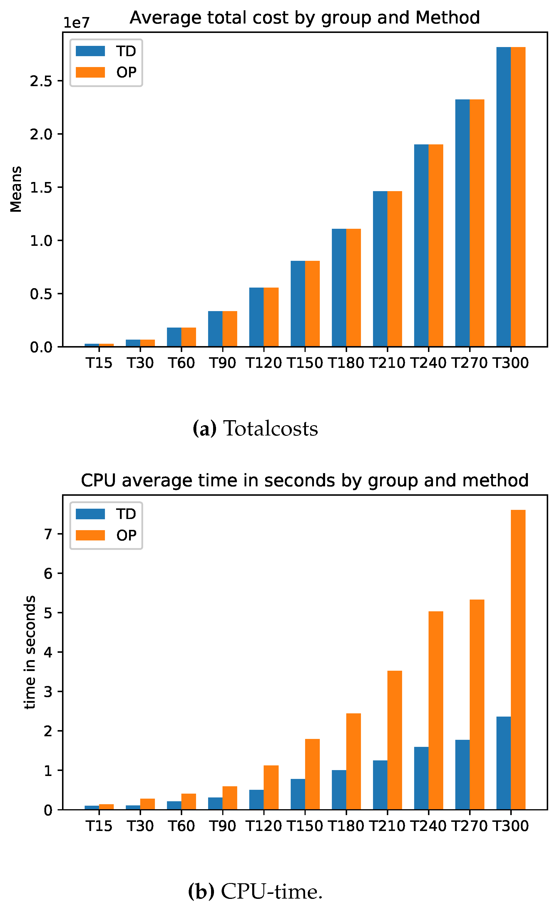
Figure A2.
Model A: Average Inventory cost.
Appendix A.2. Model B
Visualization of the results and average costs.
Figure A3.
Model B: Average Total cost and CPU time.
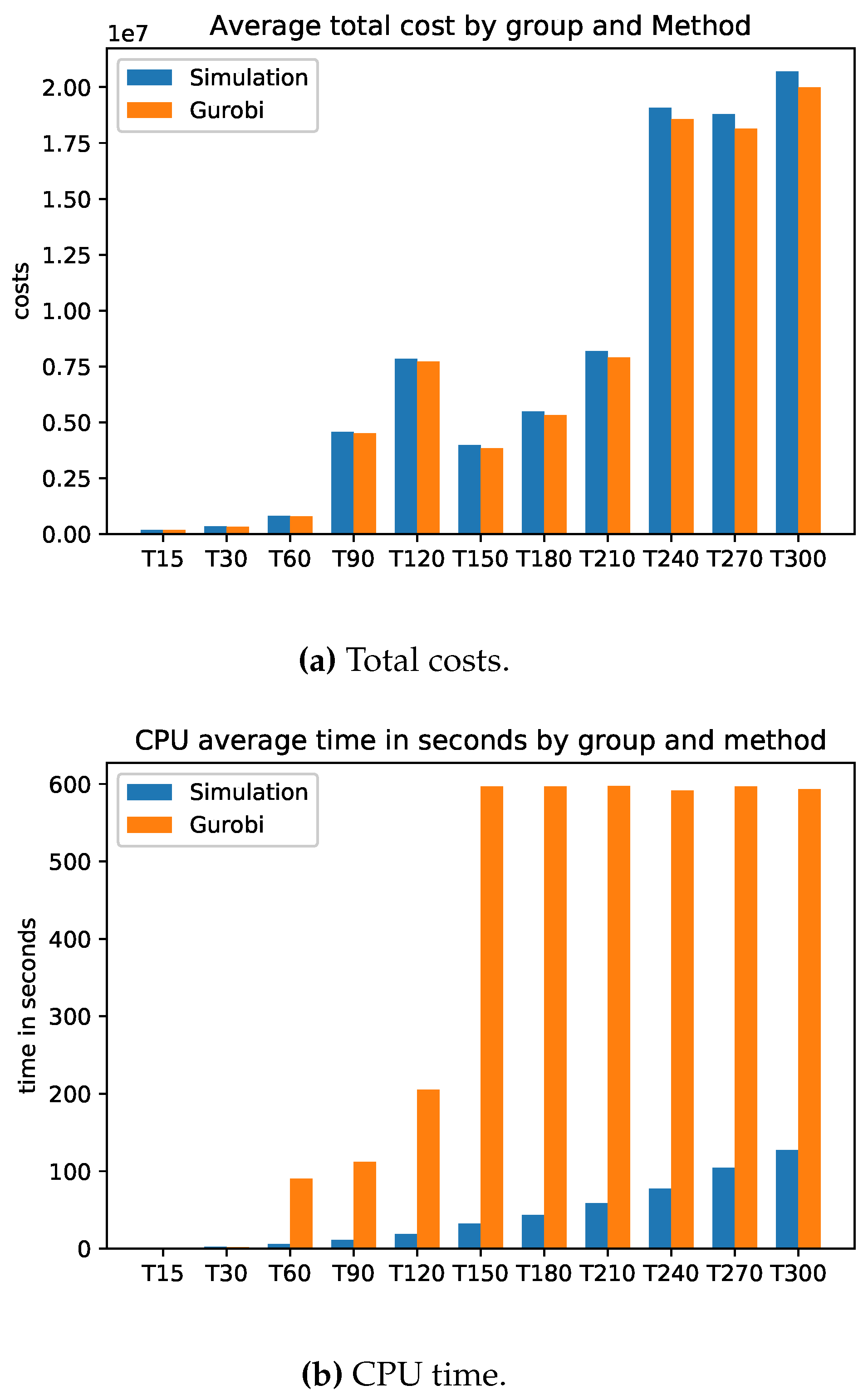
Figure A4.
Model B: Average Total cost.
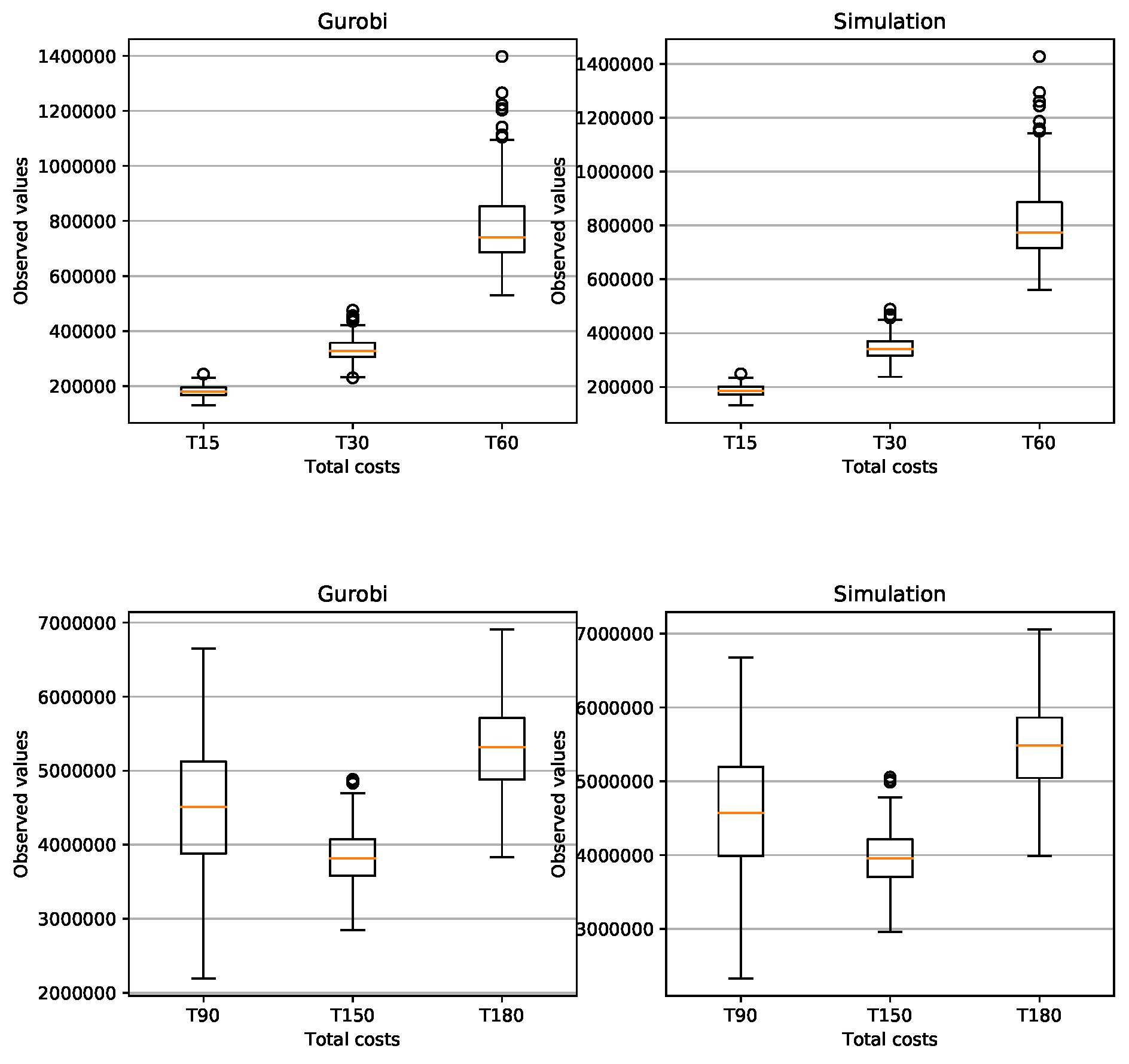
Figure A5.
Model B: Average Total cost.
Appendix B. Average Costs

Table A1.
Model A: Average Total Costs.
| Total costs | T | 15 | 30 | 60 | 90 | 120 | 150 |
|---|---|---|---|---|---|---|---|
| Count | 172 | 155 | 167 | 162 | 166 | 164 | |
| TD | Mean | 274061 | 665537 | 1798127 | 3348945 | 5552436 | 8062797 |
| Std. | 87161 | 151370 | 389288 | 660684 | 906092 | 1349699 | |
| Optimal | Mean | 268593 | 659453 | 1792494 | 3344788 | 5546715 | 8058311 |
| Std. | 83431 | 148783 | 385859 | 659403 | 904686 | 1348457 | |
| Relative error | TcError | 2.04% | 0.92% | 0.31% | 0.12% | 0.10% | 0.06% |
| Total costs | T | 150 | 180 | 210 | 240 | 270 | 300 |
| Count | 164 | 164 | 168 | 168 | 170 | 168 | |
| TD | Mean | 8062797 | 11087631 | 14620895 | 19015245 | 23243458 | 28160753 |
| Std. | 1349699 | 1811439 | 2199306 | 2911556 | 3384673 | 3870830 | |
| Optimal | Mean | 8058311 | 11081145 | 14614610 | 19008049 | 23237758 | 28154353 |
| Std. | 1348457 | 1808995 | 2198938 | 2910200 | 3382841 | 3868995 | |
| Relative error | TcError | 0.06% | 0.06% | 0.04% | 0.04% | 0.02% | 0.02% |
Table A2.
Model A: Average CPU time.
| CPU Time | T | 15 | 30 | 60 | 90 | 120 | 150 |
|---|---|---|---|---|---|---|---|
| Count | 172 | 155 | 167 | 162 | 166 | 164 | |
| TD | Mean | 0.10 | 0.11 | 0.21 | 0.31 | 0.50 | 0.78 |
| Std. | 0.06 | 0.05 | 0.10 | 0.16 | 0.26 | 0.39 | |
| Optimal | Mean | 0.14 | 0.28 | 0.41 | 0.59 | 1.12 | 1.79 |
| Std. | 0.06 | 0.11 | 0.17 | 0.30 | 0.51 | 1.42 | |
| Relative error | CPUError | -25.27% | -59.97% | -49.61% | -47.53% | -55.39% | -56.26% |
| CPU Time | T | 150 | 180 | 210 | 240 | 270 | 300 |
| Count | 164 | 164 | 168 | 168 | 170 | 168 | |
| TD | Mean | 0.78 | 1.00 | 1.25 | 1.59 | 1.77 | 2.36 |
| Std. | 0.39 | 0.47 | 0.69 | 0.82 | 0,90 | 1.39 | |
| Optimal | Mean | 1.79 | 2.44 | 3.52 | 5.03 | 5.33 | 7.60 |
| Std. | 1.42 | 1.73 | 3.00 | 3.50 | 3.98 | 5.97 | |
| Relative error | CPUError | -56.26% | -59.00% | -64.53% | -68.46% | -66.87% | -68,94% |
Table A3.
Model B: Average Total Costs.
| Total costs | T | 15 | 30 | 60 | 90 | 120 | 150 |
|---|---|---|---|---|---|---|---|
| Count | 200 | 200 | 200 | 200 | 200 | 200 | |
| Simulation | Mean | 185971 | 342933 | 815220 | 4576352 | 7829443 | 3979678 |
| Std. | 21273 | 45909 | 155884 | 858442 | 1559305 | 397507 | |
| Gurobi | Mean | 182040 | 332163 | 784654 | 4498331 | 7718552 | 3845522 |
| Std. | 21125 | 45150 | 155097 | 882996 | 1594738 | 393440 | |
| Relative error | TcError | 2.16% | 3.24% | 3.90% | 1.73% | 1.44% | 3.49% |
| Total costs | T | 150 | 180 | 210 | 240 | 270 | 300 |
| Count | 200 | 200 | 200 | 200 | 200 | 200 | |
| Simulation | Mean | 3979678 | 5477237 | 8177244 | 19065355 | 18786745 | 20708665 |
| Std. | 397507 | 593444 | 1275892 | 4030464 | 3201422 | 3672141 | |
| Gurobi | Mean | 3845522 | 5318346 | 7905438 | 18570461 | 18146172 | 19992493 |
| Std. | 393440 | 590176 | 1265172 | 4055425 | 3179322 | 3670651 | |
| Relative error | TcError | 3.49% | 2.99% | 3.44% | 2.66% | 3.53% | 3.58% |
Table A4.
Model B: Average CPU time.
| CPU Time | T | 15 | 30 | 60 | 90 | 120 | 150 |
|---|---|---|---|---|---|---|---|
| Count | 200 | 200 | 200 | 200 | 200 | 200 | |
| Simulation | Mean | 0.79 | 2.28 | 5.94 | 11.68 | 19.87 | 34.12 |
| Std. | 0.13 | 0.13 | 0.16 | 0.18 | 0.23 | 0.54 | |
| Gurobi | Mean | 0.12 | 1.57 | 90.38 | 111.93 | 204.94 | 597.03 |
| Std. | 0.08 | 1.53 | 156.10 | 186.04 | 245.47 | 36.02 | |
| Relative error | CPUError | 552.92% | 44.87% | -93.43% | -89.56% | -90.31% | -94.28% |
| CPU Time | T | 150 | 180 | 210 | 240 | 270 | 300 |
| Count | 200 | 200 | 200 | 200 | 200 | 200 | |
| Simulation | Mean | 34.12 | 46.26 | 62.84 | 77.96 | 101.69 | 130.17 |
| Std. | 0.54 | 0.58 | 1.22 | 2.63 | 2.74 | 3.78 | |
| Gurobi | Mean | 597.03 | 596.88 | 597.47 | 591.51 | 596.54 | 593.22 |
| Std. | 36.02 | 4.06 | 3.92 | 33.19 | 3.80 | 7.14 | |
| Relative error | CPUError | -94.28% | -92.25% | -89.48% | -86.82% | -82.95% | -78.06% |
Table A5.
Model B: Inventory costs.
| Inventory costs | T | 15 | 30 | 60 | 90 | 120 | 150 |
|---|---|---|---|---|---|---|---|
| Count | 200 | 200 | 200 | 200 | 200 | 200 | |
| Simulation | Mean | 28307 | 52842 | 112536 | 253095 | 340599 | 260657 |
| Std. | 5341 | 8170 | 12391 | 86118 | 107587 | 28744 | |
| Gurobi | Mean | 27801 | 57117 | 132943 | 509248 | 790970 | 318360 |
| Std. | 6907 | 12243 | 29889 | 194930 | 324335 | 43350 | |
| Relative error | Inv. Error | 1.82% | -7.49% | -15.35% | -50.30% | -56.94% | -18.13% |
| Inventory costs | T | 150 | 180 | 210 | 240 | 270 | 300 |
| Count | 200 | 200 | 200 | 200 | 200 | 200 | |
| Simulation | Mean | 260657 | 345666 | 542344 | 990715 | 1147482 | 1282444 |
| Std. | 28744 | 38613 | 75292 | 175805 | 161861 | 196713 | |
| Gurobi | Mean | 318360 | 507104 | 835915 | 1859977 | 1730800 | 1959659 |
| Std. | 43350 | 89630 | 191367 | 486708 | 372666 | 455506 | |
| Relative error | Inv. Error | -18.13% | -31.84% | -35.12% | -46.74% | -33.70% | -34.56% |
Table A6.
Model B: Return stock cost.
| Return Inv. costs | T | 15 | 30 | 60 | 90 | 120 | 150 |
|---|---|---|---|---|---|---|---|
| Count | 200 | 200 | 200 | 200 | 200 | 200 | |
| Simulation | Mean | 45867 | 92667 | 249888 | 3690209 | 6646915 | 821946 |
| Std. | 18040 | 35850 | 137395 | 1028216 | 1793396 | 208315 | |
| Gurobi | Mean | 41356 | 74641 | 195294 | 3346068 | 6070949 | 700634 |
| Std. | 17493 | 33456 | 133042 | 1109603 | 1957840 | 207573 | |
| Relative error | Ret. Inv. Error | 10.91% | 24.15% | 27.96% | 10.28% | 9.49% | 17.31% |
| Return Inv. costs | T | 150 | 180 | 210 | 240 | 270 | 300 |
| Count | 200 | 200 | 200 | 200 | 200 | 200 | |
| Simulation | Mean | 821946 | 1548362 | 2628642 | 9347966 | 7251886 | 8608929 |
| Std. | 208315 | 482657 | 1041268 | 4406311 | 2744151 | 3706917 | |
| Gurobi | Mean | 700634 | 1293559 | 2169556 | 8142232 | 6309891 | 7524531 |
| Std. | 207573 | 477084 | 1026872 | 4293352 | 2685984 | 3610684 | |
| Relative error | Ret. Inv. Error | 17.31% | 19.70% | 21.16% | 14.81% | 14.93% | 14.41% |
Table A7.
Model B: Average Setup costs.
| Setup Costs | T | 15 | 30 | 60 | 90 | 120 | 150 |
|---|---|---|---|---|---|---|---|
| Count | 200 | 200 | 200 | 200 | 200 | 200 | |
| Simulation | Mean | 50033 | 106876 | 238570 | 293071 | 388685 | 1521814 |
| Std. | 10663 | 17638 | 31424 | 27563 | 34664 | 212705 | |
| Gurobi | Mean | 55707 | 114588 | 248504 | 307481 | 408104 | 1458747 |
| Std. | 10343 | 17268 | 30443 | 27399 | 37230 | 201433 | |
| Relative error | Setup. Error | -10.19% | -6.73% | -4.00% | -4.69% | -4.76% | 4.32% |
| Setup Costs | T | 150 | 180 | 210 | 240 | 270 | 300 |
| Count | 200 | 200 | 200 | 200 | 200 | 200 | |
| Simulation | Mean | 1521814 | 1699197 | 2214098 | 2828660 | 3716988 | 4920930 |
| Std. | 212705 | 233148 | 330991 | 404730 | 467555 | 902775 | |
| Gurobi | Mean | 1458747 | 1641182 | 2118141 | 2669355 | 3397775 | 4526298 |
| Std. | 201433 | 223689 | 310292 | 367954 | 412785 | 200 | |
| Relative error | Setup. Error | 4.32% | 3.53% | 4.53% | 5.97% | 9.39% | 8.72% |
| 1 | We can always transform a problem with non zero initial or final stock by adapting the demand. |
| 2 | low discrepancy sequences are called quasi-random sequences. |
| 3 | The test instances and solutions are available here. |
References
- Manne, A.S. Programming of economic lot sizes. Management science 1958, 4, 115–135. [Google Scholar] [CrossRef]
- Wagner, H.M.; Whitin, T.M. Dynamic version of the economic lot size model. Management science 1958, 5, 89–96. [Google Scholar] [CrossRef]
- Beltrán, J.L.; Krass, D. Dynamic lot sizing with returning items and disposals. IIe transactions 2002, 34, 437–448. [Google Scholar] [CrossRef]
- Elmaghraby, S.E. The Economic Lot Scheduling Problem (ELSP): Review and Extensions. Management Science 1978, 24, 587–598. [Google Scholar] [CrossRef]
- Brahimi, N.; Dauzere-Peres, S.; Najid, N.M.; Nordli, A. Single item lot sizing problems. European Journal of Operational Research 2006, 168, 1–16. [Google Scholar] [CrossRef]
- Buschkühl, L.; Sahling, F.; Helber, S.; Tempelmeier, H. Dynamic capacitated lot-sizing problems: a classification and review of solution approaches. Or Spectrum 2010, 32, 231–261. [Google Scholar] [CrossRef]
- Thierry, M.; Salomon, M.; Van Nunen, J.; Van Wassenhove, L. Strategic issues in product recovery management. California management review 1995, 37, 114–136. [Google Scholar] [CrossRef]
- Amin, S.H.; Zhang, G.; Eldali, M. A review of closed-loop supply chain models. Journal of Data, Information and Management 2020, 2, 279–307. [CrossRef]
- Agrawal, S.; Singh, R.K.; Murtaza, Q. A literature review and perspectives in reverse logistics. Resources, Conservation and Recycling 2015, 97, 76–92. [CrossRef]
- Ayres, R.; Ferrer, G.; Van Leynseele, T. Eco-efficiency, asset recovery and remanufacturing. European Management Journal 1997, 15, 557–574. [Google Scholar] [CrossRef]
- Inderfurth, K. Optimal policies in hybrid manufacturing/remanufacturing systems with product substitution. International Journal of Production Economics 2004, 90, 325–343. [Google Scholar] [CrossRef]
- Tang, O.; Teunter, R. Economic lot scheduling problem with returns. Production and Operations Management 2006, 15, 488–497. [Google Scholar] [CrossRef]
- Teunter, R.; Kaparis, K.; Tang, O. Multi-product economic lot scheduling problem with separate production lines for manufacturing and remanufacturing. European journal of operational research 2008, 191, 1241–1253. [Google Scholar] [CrossRef]
- Sahling, F. A Column-Generation Approach for a Short-Term Production Planning Problem in Closed-Loop Supply Chains. BuR- Business Research 2013, 6(1), 55–75. [CrossRef]
- Cunha, J.O.; Konstantaras, I.; Melo, R.A.; Sifaleras, A. On multi-item economic lot-sizing with remanufacturing and uncapacitated production. Applied Mathematical Modelling 2017, 50, 772–780. [Google Scholar] [CrossRef]
- Sifaleras, A.; Konstantaras, I. Variable neighborhood descent heuristic for solving reverse logistics multi-item dynamic lot-sizing problems. Electronic Notes in Discrete Mathematics 2015, 47, 69–76. [Google Scholar] [CrossRef]
- Cunha, J.O.; Kramer, H.H.; Melo, R.A. Effective matheuristics for the multi-item capacitated lot-sizing problem with remanufacturing. Computers & Operations Research 2019, 104, 149–158. [CrossRef]
- Helmrich, R.; Jans, M.; van den Heuvel, W.; Wagelmans, A. Economic lot-sizing with remanufacturing: Complexity and efficient formulations. IISE Transactions 2014, 46(1), 67–86. [Google Scholar] [CrossRef]
- Kilic, O.; van den Heuvel, W. Economic lot sizing with remanufacturing: Structural properties and polynomial-time heuristics.IISE Transactions 2019,51:12, 1318–1331. [CrossRef]
- Richter, K.; Weber, J. The reverse Wagner/Whitin model with variable manufacturing and remanufacturing cost. International Journal of Production Economics 2001, 71, 447–456. [Google Scholar] [CrossRef]
- Richter, K.; Sombrutzki, M. Remanufacturing planing for the reverse Wagner/Whitin models. Journal of Operational Research 2000, 121, 304–315. [Google Scholar] [CrossRef]
- Teunter, R.; Bayindir, Z.; van den Heuvel, W. Dynamic lot sizing with product returns and remanufacturing. Int. Journal of Production Research 2006, pp. 4377–4400. [CrossRef]
- Schulz, T. A new Silver-Meal basic heuristic for the single-item dynamic lot sizing problem with returns and remanufacturing. International Journal of Production Research 2011, p. 2519–2533. [CrossRef]
- Cunha, J.; Melo, R. A computational comparison of formulations for the economic lot-sizing with remanufacturing. Computers & Industrial Engineering 2016, 92, 72–81. [CrossRef]
- Piñeyro, P.; Viera, O. The economic lot-sizing problem with remanufacturing and heterogeneous returns: formulations, analysis and algorithms. International Journal of Production Research 2022, 60, 3521–3533. [Google Scholar] [CrossRef]
- Lahmar, H.; Dahane, M.; Mouss, K.; Haoues, M. Multi-objective production planning of new and remanufactured products in hybrid production system. IFAC-PapersOnLine 2022, 55, 275–280. [CrossRef]
- Zouadi, T.; Yalaoui, A.; Reghioui, M. Lot sizing and pricing problem in a recovery system with returns and one-way substitution option: Novel cost benefit evaluation based approaches. IFAC-PapersOnLine 2019, 52, 36–41. [CrossRef]
- Şenyiğit, E.; Erol, R. New lot sizing heuristics for demand and price uncertainties with service-level constraint. International Journal of Production Research 2010, 48, 21–44. [Google Scholar] [CrossRef]
- Zhang, Z.H.; Jiang, H.; Pan, X. A Lagrangian relaxation based approach for the capacitated lot sizing problem in closed-loop supply chain. International Journal of Production Economics 2012, 140, 249–255. [Google Scholar] [CrossRef]
- Florian, M.; Lenstra, J.K.; Rinnooy Kan, A. Deterministic production planning: Algorithms and complexity. Management science 1980, 26, 669–679. [Google Scholar] [CrossRef]
- Bitran, G.R.; Yanasse, H.H. Computational complexity of the capacitated lot size problem. Management Science 1982, 28, 1174–1186. [Google Scholar] [CrossRef]
- Dixon, P.S. Multi-Item Lot-Sizing with Limited Capacity. dissertation, University of Waterloo, Ontario, 1979.
- Dziuba, D.; Almeder, C. New construction heuristic for capacitated lot sizing problems. European Journal of Operational Research 2023. [Google Scholar] [CrossRef]
- Maes, J.; McClain, J.; Van Wassenhove, L. Multilevel capacitated lotsizing complexity and LP-based heuristics. Journal of Operational Research 1991, 53, 131–148. [Google Scholar] [CrossRef]
- Sobol’, I.M. Calculation of improper integrals using uniformly distributed sequences. Soviet Math. Dokl. 1973, 14, 734–738. [Google Scholar]
- Halton, J.H. On the efficiency of certain quasi-random sequences of points in evaluating multi-dimensional integrals. Numerische Mathematik 1960, 2, 84–90. [Google Scholar] [CrossRef]
- Niederreiter, H. Quasi-Monte Carlo methods and pseudo-random numbers. Bull. Am. Math. Soc. 1978, 84, 957–1041. [Google Scholar] [CrossRef]
- Klinger, B. Numerical integration of singular integrands using low-discrepancy sequences. Computing 1997, 59, 223–236. [Google Scholar] [CrossRef]
- Van den Heuvel, W.; Wagelmans, A.P. Four equivalent lot-sizing models. Operations Research Letters 2008, 36, 465–470. [Google Scholar] [CrossRef]
- Maes, J.; Van Wassenhove, L. A simple heuristic for the multi item single level capacitated lotsizing problem. Operations research letters 1986, 4, 265–273. [Google Scholar] [CrossRef]
- Knuth, D.E. Art of computer programming: Seminumerical algorithms; Vol. 2, Addison-Wesley Professional, 2014.
- von Neumann, J. Various techniques used in connection with random digits. Monte Carlo Method, Appl. Math. Series 1951, 12, 36–38.
- Niederreiter, H. Random number generation and quasi-Monte Carlo methods; SIAM, 1992.
- Tezuka, S. Uniform random numbers: Theory and practice; Vol. 315, Springer Science & Business Media, 2012.
- Chaitin, G.J. Information, Randomness and Incompleteness. Papers on Algorithmic Information Theory. 1987, p. 236. , p. 236.
- Kolmogorov, A.N.; Uspenskii, V.A. Algorithms and randomness. Theory of Probability & Its Applications 1988, 32, 389–412. [CrossRef]
- Schnorr, C. Zufälligkeit und Wahrscheinlichkeit. Lecture Notes in Math. 1971, 218, 109. [Google Scholar]
Figure 1.
Dynamic Capacitated Lot-Sizing with Produkt Returns and Remanufacturing.
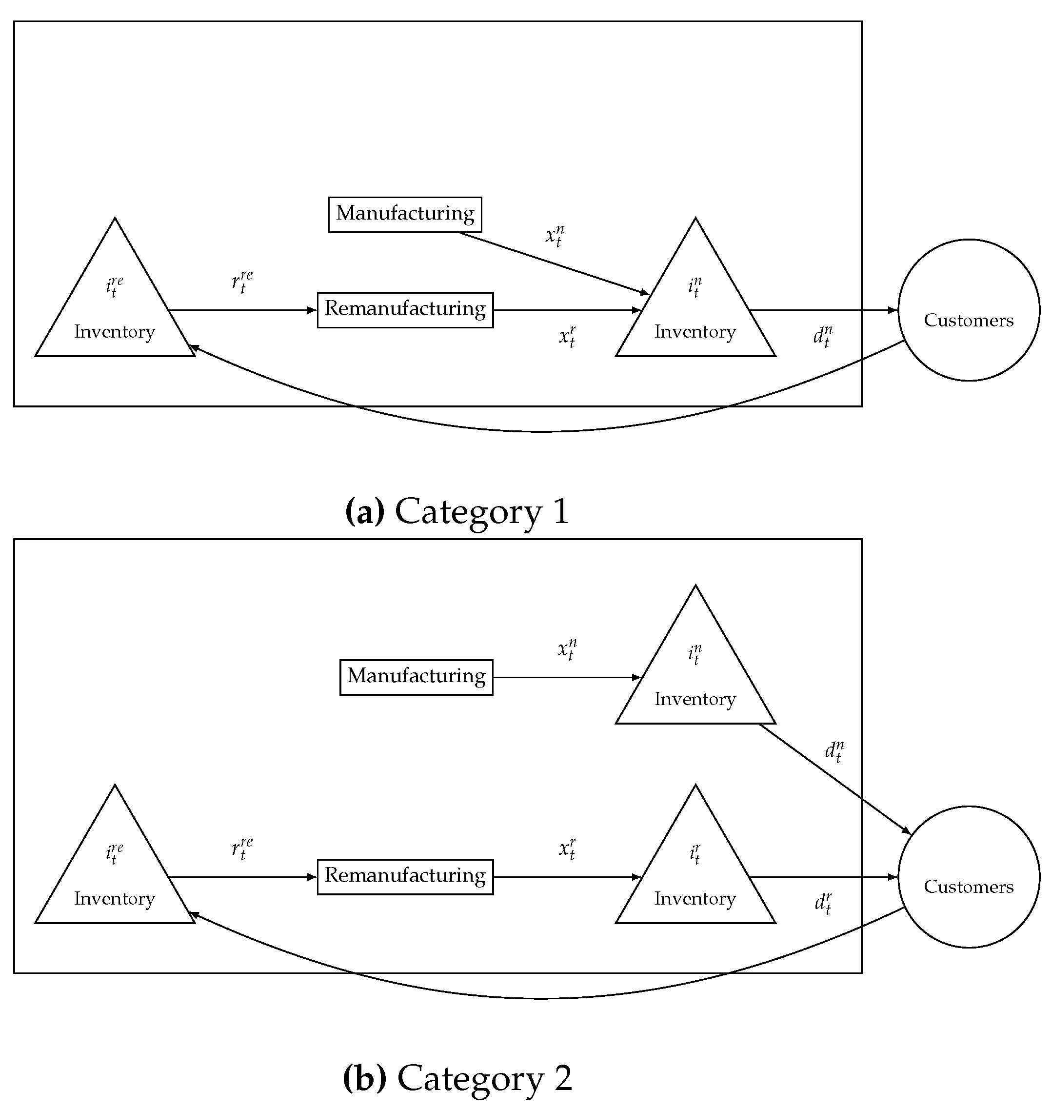
Figure 2.
Two-dimensional projection of 5000 Halton and Pseudorandom points.
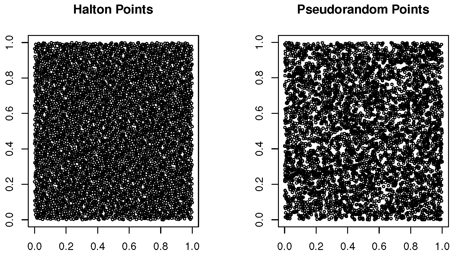
Table 1.
Data and parameters
| Name | Paramenter |
|---|---|
| T | Number of time periods |
| Initial inventory stocks | |
| Cost per unit and period t | |
| Setup cost for manufacturing new product | |
| Setup cost for remanufacturing product | |
| production cost of new product | |
| production cost of remanufactured product | |
| holding cost of new product | |
| holding cost of remanufactured product | |
| holding cost of returned product | |
| Demand and return in period t | |
| Demand of new product | |
| Demand of remanufactured product | |
| Quantity of returned product | |
| Available Capacities in period t | |
| capacities for manufacturing and | |
| remanufacturing | |
| (capacity requirement for new product and | |
| recovery product is set to one). | |
Table 2.
Decision variables
| Name | Paramenter |
|---|---|
| 1, if new products are manufactured | |
| in period t; 0, otherwise | |
| quantity of new products manufactured | |
| in period t | |
| inventory stock of new products | |
| at the end of period t | |
| 1, if returned products are remanufactured | |
| in period t; 0, otherwise | |
| quantity of returned products remanufactured | |
| in period t | |
| inventory stock of remanufactured | |
| products at the end of period t | |
| inventory stock of returned products | |
| at the end of period t |
Table 3.
Original Data
| t | w | |||||
|---|---|---|---|---|---|---|
| 1 | 198 | 153 | 183 | 336 | 609 | 57 |
| 2 | 806 | 84 | 302 | 386 | 632 | 246 |
| 3 | 223 | 100 | 146 | 246 | 101 | -145 |
| 4 | 283 | 100 | 127 | 227 | 295 | 68 |
| 5 | 500 | 248 | 598 | 846 | 620 | -226 |
| 6 | 500 | 0 | 0 | 0 | 561 | 0 |
| Sum | 2510 | 685 | 1356 | 2041 | 2818 | 0 |
Table 4.
Demand Transformation
| t | ||||||
|---|---|---|---|---|---|---|
| 1 | 195 | 198 | 393 | 609 | 393 | 609 |
| 2 | 42 | 590 | 632 | 632 | 1025 | 1241 |
| 3 | 101 | 0 | 101 | 101 | 1126 | 1342 |
| 4 | 295 | 0 | 295 | 295 | 1421 | 1637 |
| 5 | 52 | 568 | 620 | 620 | 2041 | 2257 |
| 6 | 0 | 0 | 0 | 561 | 2041 | 2818 |
| Sum | 685 | 1356 | 2041 | 2818 |
Table 5.
Halton Numbers.
| Prime numbers | ||||
|---|---|---|---|---|
| 2 | 3 | 5 | 7 | |
| n | Halton numbers | |||
| 1 | 0,5 | 0,33333333 | 0,2 | 0,14285714 |
| 2 | 0,25 | 0,66666667 | 0,4 | 0,28571429 |
| 3 | 0,75 | 0,11111111 | 0,6 | 0,42857143 |
| 4 | 0,125 | 0,44444444 | 0,8 | 0,57142857 |
| 5 | 0,625 | 0,77777778 | 0,04 | 0,71428571 |
Table 6.
Problem classes.
| PC1 | PC2 | PC3 | PC4 | PC5 | PC6 | |
|---|---|---|---|---|---|---|
| T | 15 | 30 | 60 | 90 | 120 | 150 |
| PC7 | PC8 | PC9 | PC10 | PC11 | ||
| T | 180 | 210 | 240 | 270 | 300 |
Table 7.
Parameters for Model A.
| with condition (1) | |
| with condition (4) | with condition (3) |
| = | |
| = | |
| represent the average demand values. |
Table 9.
Schematic of the simulation.
| Step 1 | Initialisation:, |
| Step 2 | If stop; otherwise go to Step 3. |
| Step 3 | Using Algorithms 3 and 4 along with calculate the function |
| Step 4 | If then . |
| Step 5 | and go to Step 2. |
Disclaimer/Publisher’s Note: The statements, opinions and data contained in all publications are solely those of the individual author(s) and contributor(s) and not of MDPI and/or the editor(s). MDPI and/or the editor(s) disclaim responsibility for any injury to people or property resulting from any ideas, methods, instructions or products referred to in the content. |
© 2024 by the authors. Licensee MDPI, Basel, Switzerland. This article is an open access article distributed under the terms and conditions of the Creative Commons Attribution (CC BY) license (http://creativecommons.org/licenses/by/4.0/).
Copyright: This open access article is published under a Creative Commons CC BY 4.0 license, which permit the free download, distribution, and reuse, provided that the author and preprint are cited in any reuse.


