Submitted:
03 April 2023
Posted:
03 April 2023
You are already at the latest version
Abstract
Semi-structured complex numbers H was a number set developed to enable division by zero in ordinary algebraic equations. Its utility has been shown in mathematics and engineering. However, very little has been done to show its usefulness in computer science. Consequently, the aim of this paper was to show the utility of semi-structured complex numbers in computer science by developing a division by zero calculator. First two computer programs were written, one for a standard (STD) calculator and the other for a division by zero (DBZ) calculator. The programs were fed 20000 randomly generated arithmetic equations of varying lengths and the space and time complexity associated with processing these equations were measured and compared to determine the efficiency of each calculator. In the process, three major contributions were made: (1) A representation for semi-structured complex numbers that enables it to be easily used by a computer was developed; (2) It was demonstrated that the DBZ calculator outperforms the STD calculator in terms of efficiency; and, (3) It was shown that the number set H reduced the amount of error handling required to run a computer program. These results provide a firm foundation to advance the number set as a useful tool in computer science.
Keywords:
Semi-structured complex numbers
; Division by zero
; computer science
; Calculator
; Exception handling
1. Introduction
1.1. Semi-structured complex numbers: a recent development in division by zero
Recently there has been a range of research involving division by zero. Table 13, Appendix 1, shows sample of such research conducted from 2018 to 2022 on “division by zero” including using division by zero to explain cancer development. The problem of division by zero can simply be stated as: What is where “a” is any complex number. There have been several solutions to the problem the most recent being the invention of the semi-structured complex number set [1]. The first attempt at creating this number set was riddled with issues [1], however, a second paper [2] was written to reformulate and strengthen the theory of semi-structured complex numbers and in the process produced several profound results. Table 1 shows the major results developed in paper [2].
Results 1 to Result 9 in Table 1 provide some significant foundational results for semi-structured complex numbers. Nevertheless, it is necessary to go beyond just the foundational setting and look at how this new number set can be applied in a practical setting particularly in the area computer science where real world problems are constantly being modelled and solved using mathematical tools.
1.2. Potential importance of Semi-structured complex numbers to computer science
Computers are generally run on computer programs (software). On a fundamental level these computer programs consist largely of arithmetic and logic operations. In writing and running a computer program, errors can occur. These errors are often called “exceptions”.
An exception is an event, which occurs during the execution of a program, that disrupts the normal flow of the program's instructions [3]. There are several types of program exceptions one of the most fundamental being a Run-time exception. Examples of this type of exception include a user entering invalid input into a program or a program attempting to divide by zero [4].
If a program has several statements and an exception happens midway through its execution, the statements after the exception do not execute, and the program crashes. To prevent this, exceptions are usually handled in a process called “Exception Handling”. In exception handling specialised computer program instructions are used to tell the computer program what to do if an exception occurs. An example of such instructions is the popular “try-catch blocks” (or some variation of this) used in many programming languages. This is shown in Figure 1.
The "Try block” is a computer instruction that detects the exception (or error) during program execution and the “Catch block” tells the computer program what to do to deal with (or handle) the exception or error. Although exception handling is common practice in computer programs, they do have several disadvantages. These are given in Table 2.
Since most computer programs use real and or complex number arithmetic in their operations, “division by zero” can caused Run-time exceptions. Considering the disadvantages listed in Table 2, it would be ideal to reduce run-time exceptions caused by “division by zero”. This can easily be done if semi-structured complex numbers are used in computer programming.
However, proving the utility of such numbers in computer programming requires comparing the performance of a computer program when semi-structured numbers are implemented in that program verses when exception handling is used instead. Very little has been done to show such a comparison.
1.3. Semi-structured complex numbers and a division by zero calculator
One of the simplest programs that can be written to show the utility of semi-structured complex numbers is an arithmetic calculator program.
In the standard arithmetic calculator, users can enter valid arithmetic equations and the calculator produces a result. Equations are generally entered in what is called “infix notation”. Infix notation operators such as lies between a pair of operands (numbers or letters). An example of infix notation is .
The calculator converts the infix notation into postfix notation. In postfix notation the operator is followed by every pair of operands. For example, in postfix notation becomes . The calculator then evaluates the postfix expression. Table 3 provides three further examples of infix and postfix expressions.
Infix expressions are readable and solvable by humans who can easily distinguish the order of operators and use the parenthesis to solve parts of equations before others. Computer calculators have difficulty efficiently evaluating infix expressions (being unable to differentiate between parenthesis and operators). Therefore, infix expressions are generally converted to postfix form and then evaluated by the calculator.
Arithmetic equations entered by the user can easily contain division by zero. In standard arithmetic calculators whenever division by zero occurs the program halts and some exception handling occurs. It would be instructive to write a standard arithmetic calculator that can perform division by zero operations to determine how well the program would perform under thousands of random calculations including calculations involving division by zero. Such a calculator would need to be made to execute arithmetic operations on semi-structured complex numbers. However, very little has been done to pursue such an endeavour.
1.4. Measuring the performance of a division by zero calculator
When creating a computer program, it is important to measure the performance of the computer program against some standard or benchmark. In such cases performance metrices and a well-known benchmark are needed.
In general, the performance of a computer program is measured in terms of its efficiency. Algorithm efficiency relates to how many resources a computer needs to expend to process an algorithm. When creating an algorithm, it is important to make it as streamlined as possible, so it does not strain the software or device that runs it. If an algorithm is not efficient, it is not considered fit for its purpose. Two main measures of algorithm efficiency are space complexity and time complexity. Space complexity measures how much memory is used to process the input and output of the algorithm as well as the algorithm itself [6]. On the other hand, the time complexity measures how long it takes to process the algorithm [7].
Space complexity is the measurement of total space required by an algorithm to execute properly. For example, the input memory space complexity can simply be a measure of the size of the file (in bytes or kilobytes) containing the input data for the program. Likewise, the output space complexity can be a measure of the size of the file (in bytes of kilobytes) containing the output data for the program. The amount of memory required to run a program can be measured in many ways. The best algorithm should have a low level of space complexity. The less space required, the faster it executes.
Most computer languages generally have functions (special computer instructions) to measure time complexity for a computer program. For example, in Python (one of the most popular computer languages used today) functions such as time.start() and time.stop() are placed before and after a computer program respectively and are used to measure the start and stop times for a computer program. Subtracting the values produced by these functions gives the runtime of the computer program. When comparing two algorithms to solve the same problem, the algorithm with the smaller time complexity is considered the better of the two algorithms. To show that the division by zero calculator is useful it must outperform a standard arithmetic calculator in terms of efficiency (that is, in terms of the space and time complexity).
1.5. Major Contributions of this research
Given the potential importance of semi-structured complex numbers in computer science, the aim of this paper was:
To demonstrate the utility of semi-structured complex numbers in computer science by developing a division by zero calculator.
In the process of achieving the stated aim, the following major contributions are made in this paper:
- 1.
- A representation for semi-structured complex numbers that enables it to be easily used in arithmetic operations by a computer program was developed. The semi-structured complex numbers is represented by the 3-tuple (or ordered triple) given by .
- 2.
- It was demonstrated that the division by zero calculator outperforms the standard calculator in terms of efficiency (that is space and time complexity).
- 3.
- It was shown that the number set reduced the amount of error handling required to run a computer program.
The rest of this paper is devoted to providing a detailed explanation of how the major contributions outlined were arrived at.
2. Method
2.1. Representing semi-structured complex numbers for use in a computer program
The first step was to represent a typical semi-structured complex number in a simple form that can be used in a computer program. In this case, the computer program would be an arithmetic calculator. The typical semi-structured complex number has the form:
Here are real numbers. The numbers are the important aspects of the semi-structured complex numbers. For the calculator created in this paper, the semi-structured complex number can simply be represented as a triple written as . Hence:
The format shown in Equation (4) is called semi-structured complex triple format. More examples of this format are given in Table 4.
The advantage of this format is that it is unambiguous in terms of meaning and very little space is required to store a semi-structured complex number.
2.2. Develop a semi-structured complex numbers equation generator
With the representation of semi-structured complex numbers given in Equation (4) it is now simple to generate arithmetic equations that can be used to evaluate the efficiency of a calculator. Hence, an equation generator was developed to create equations to be evaluated by both a standard and a division by zero calculator. The equations produced are random but valid infix equations consisting of operators () and semi-structured complex number operands that have the form . Collectively, these operators and operands are called tokens. The rules for generating a random arithmetic equation are simple:
- i.
- Generate a random odd number greater than or equal to three. The random odd number indicates the number of tokens (arithmetic operators and operands) that the equation would have. The number of tokens must be a minimum of three tokens, that is, an operand followed by an operator followed by another operand. Every valid equation greater than three tokens in length will have an odd number of tokens.
- ii.
- Every equation must start and end with an operand.
- iii.
- Operators were always in even positions within the infix expression and operands always in odd positions.
- iv.
- For the sake of simplicity brackets were not produced in the infix expressions, instead the precedence of operators indicated the order in which operators were to be evaluated.
With these rules, the algorithm for the semi-structured complex numbers equation generator is given in Table 5. From Table 5 the variables, (minimum operand value, maximum operand value) in line 1 of the algorithm represented the range of numbers used in the semi-structured complex triple . Each component of the triple will have an integer value that falls within the range (minimum operand value, maximum operand value). This gives the user control of the values in the semi-structured complex number triples. Additionally, equation length (L) represented the length of the equation to be generated. This number must always be odd.
2.3. Developing common algorithms for calculator programs
Both the division by zero calculator and the standard calculator share the same basic algorithms and only differ in the way they handle the division by zero operation. These algorithms are discussed here in turn.
2.3.1. The Postfix Convertor
Once the algorithm for the equation generator was created the next step was to create an infix to postfix evaluator. The algorithm for the infix to postfix evaluator is given in Table 14 in Appendix 2. From Table 14 the variable “Operator stack” is a stack used to store the operands as the algorithm runs. A stack can be thought of as a container where operators and operands can be placed (pushed) on top of each other. Only the token on top of the stack can be removed (or popped) first. Users of a stack can also see (or peek) the token at the top of the stack without removing the top token.
2.3.2. The Postfix Evaluator
Once the equation generated has been converted from infix to postfix format, the postfix expression must be evaluated. The general postfix evaluator is given in Table 15 in Appendix 2. The primary part of the postfix evaluator is the “Arithmetic Machine” which performs the actual arithmetic on the operand given to the postfix evaluator.
2.4. Developing an Arithmetic Machine for a standard and a division by zero calculator
Two “Arithmetic Machines” were developed for this research. The first was an arithmetic machine for the standard calculator “Arithmetic Machine STD” and the second was an arithmetic machine for the division by zero calculator “Arithmetic Machine DBZ”.
A standard arithmetic calculator has only 4 basic operations addition, subtraction, multiplication, and division. Modern calculators will show an error message when division by zero is performed. In which case the user of the calculator must reset the calculator before the calculator can be used to perform another arithmetic operation.
In the standard calculator developed for this paper when the calculator faces a division by zero operation it will output an error and the calculator will use a try-catch statement to deal with the division by zero error. The try catch statement will show an error message and reset the calculator for the next equation to be processed. This operation is part of the “Arithmetic Machine STD” given in Table 7 for the standard calculator. The “Arithmetic Machine STD” given in Table 7 takes two semi-structured complex numbers and and performs one of the simple arithmetic operations on these numbers.
In the algorithm shown in Table 7, the try catch statement for division by zero is given in lines 7 to line 8. If the second operand is not zero, then the try catch statement is not executed and the algorithm continues to line 9. The algorithm also has a “Multiply” function in line 11 and line 13. This function is given in Table 16 in Appendix 2. This “Multiply” function multiplies two semi-structed complex numbers according to the normal rules of multiplication for semi-structured complex numbers given in paper [2].
The “Arithmetic Machine DBZ” algorithm for the division by zero calculator was similar to the algorithm shown in Table 7. However, the “Arithmetic Machine DBZ" handles division by zero differently as shown in Table 8.
In the algorithm shown in Table 8, if the second operand is zero, then the algorithm simply changes the second operand (line 7) to the unstructured unit value (represented as the triple 0,0,1 in semi-structured complex number format shown in Equation (4)) where . The algorithm then goes on to use the “Multiply” function in line 10. This function is given in Table 16 in Appendix 2.
The final general algorithm for both the standard calculator and the division by zero calculator is given in Table 9.
All the algorithms discussed thus far was developed and executed on an online Python platform [8]. The speed of the platform was largely dependent on the speed of the servers on which the platform was ran. Since both calculators was ran from this platform, it provided a uniform starting point to evaluate their efficiency.
2.5. Simulation procedure to compare standard and division by zero calculator
To determine the efficiency of the standard calculator and the division by zero calculator, the space and time complexity of both calculators were compared. The measures for space and time complexity are given in Table 10.
To begin, the space complexity for the standard calculator was first examined. This was done by examining the processing and output memory involved in running the standard calculator. The standard calculator was put through 20 simulations.
For the first simulation, 1000 equations were randomly generated (equation generator is given in Table 5) with each equation having a length (L) of 5 tokens. The 5 tokens consisted of 2 operators chosen at random from the group and Three operands in the form with each component of the operand being integers generated within the range to . The range was kept small to increase the probability that there was division by zero operations within the set of 1000 equations.
The average number of operations per equations was found using the equation , where L is the length of the equation (number of tokens). This value was recorded as the variable “No. of operations per equation”.
In the process of generating the equations the number of equations with division by zero was calculated and recorded as the variable “No. of Equations with division by zero operations”. This was calculated by parsing each equation to determine if it had the subsequence “/ 0,0,0”. If the subsequence existed, then the equation was recorded as having a division by zero operation.
Additionally, the number of division by zero operations that exist across all 1000 equations was calculated and recorded in the variable “Total no. of division by zero operations”. The “No. of operations per equation”, “No. of Equations with division by zero operations” and “Total no. of division by zero operations” represent the characteristics of the equations that was processed by the standard calculator.
The 1000 equations were fed into the standard calculator algorithm (shown in Table 9 with the user input for type of “Arithmetic machine” set to 1), and the total memory used to process all the equations was calculated and recorded. This was done using the Python functions tracemalloc.start() and tracemalloc.stop(). The result was recorded in the variable “Total Processing Memory”. The total number of equations successfully calculated (that is equations that did not throw any exception errors) was recorded in the variable “No. of equations successfully computed”.
The average processing memory per operation was calculated then recorded. This was done using the following formula given in Equation (5). This value was recorded as “Average Processing Memory Per operation”.
In cases where an equation had division by zero in the standard calculator, the calculator did not compute a result but threw an exception and an error message was displayed and recorded as output.
After calculating the result of each equation, the output of the results of all 1000 equations were recorded in a text file. The total output memory (the size of the text file in bytes) was then recorded.
Once the space complexity of the standard calculator was examined the time complexity for the calculator was also examined. The total time taken to process all 1000 equations for the first simulation was calculated using the Python functions time.start() and time.stop(). The function time.start() was placed at the beginning of the standard calculator function to start measuring processing time and time.stop() was placed at the end of the standard calculator function to end the measurement. The time taken to process one equation was given by Equation (6).
The total time taken to process all 1000 equations was recorded as “Total Processing Time”. The number of operations successfully computed by the standard calculator per unit time was calculated using Equation (7).
The result was recorded as “No. of operations per unit time”.
Once the space and time complexity for the standard calculator for the first simulation was determined, the process of calculating the characteristics of the equations, the space complexity and the time complexity of the standard calculator was repeated for 19 more simulations. For each simulation the length (L) of the equations was increased by 10 tokens from the previous simulation. The results were then tabulated.
The entire process of calculating the characteristics of the equations, the space and time complexity for 20 simulations of 1000 equations was repeated for the division by zero calculator. The results were then tabulated.
After the results were tabulated for the standard calculator and the division by zero calculator, three graphs were drawn. The first graph was a graph of “Average processing Memory per operation vs. Number of division by zero operations”. This graph was meant to determine how processing memory was affected by the presence of division by zero operation.
The second graph was a graph of “Total Output memory vs. Number of equations with division by zero”. This graph was meant to determine how the two calculators handle division by zero affected the amount of memory needed to output the results.
Finally, a graph of “Number of operations per unit time vs. Total number of operations” was plotted. The first two graphs provide a deeper look at the space complexity of the two calculators, whilst the final graph provides a closer look at the time complexity of the calculators.
3. Results
Table 11 and Table 12 shows the results of the simulations conducted on both the standard calculator and the division by zero calculator respectively. From Table 11 and Table 12 as the length of the equations increased the number of operations per equation, number of equations with division by zero, and total number of divisions by zero operations also increased. This implies that the complexity of the equations increased with each successive set of simulations. The space and time complexity columns indicated how well each type of calculator handled the increase in equation complexity.
In terms of space complexity, the total processing memory required to process the 1000 equations per calculator was slightly less with the standard calculator and more with the division by zero calculator. This is probability due to the standard calculator having less to process than the division by zero calculator. Recall that the standard calculator could not process division by zero calculations or division by zero equations. This is clearly seen in the final column of Table 11. Here the standard calculator only processed between 563 to 975 equations out of the 1000 equations given to it across the 20 simulations.
However, when the graph of “Average processing memory per operation vs. Total number of divisions by zero operation” it was clear that the average memory per operation was lower with the division by zero calculator. This implies that there were more successful operations per unit of memory with the division by zero calculator than with the standard calculator as the number of operations (specifically division by zero operations) increases. This is clearly seen in Figure 2.
Additionally, from Table 11 and Table 12 when the total memory output was considered it was clear that the division by zero calculator required less memory to output its results as the complexity of the equations increased (and the number of division by zero operations). This is very likely because every time the standard calculator encountered a division by zero operation it would output an error message (which required more output space than printing a simple numerical answer). Figure 3 illustrates this point more clearly.
When “Total output memory vs. Number of Equations with Division by Zero” is plotted for both the division by zero and standard calculator it was clear that the division by zero calculator outperformed the standard calculator requiring significantly less memory to output its results as the number of division by zero operations increases. Therefore overall, in terms of space complexity, the division by zero calculator outperformed the standard calculator.
Turning attention to time complexity, from Table 11 and Table 12 when the Total Processing Time is considered, the standard calculator showed a smaller time spent processing the equations. Nevertheless, the lower processing time for the standard calculator can be attributed to the fact thar the standard calculator successfully processed less equations than the division by zero calculator.
The difference in time complexity between the two calculators is more clearly seen in Figure 4, when the “Number of operations per unit time against the Total Number of operations” is compared for both calculators.
Clearly from Figure 4, the division by zero calculator was able to process more successful operations per unit time than the standard calculator (this considering that the division by zero calculator was able to successfully process division by zero operations). Therefore, in terms of time complexity the division by zero outperformed the standard calculator.
From the overall results it was also clearly seen that removing the try catch statements to handle division by zero exceptions improved the efficiency of a calculator program. Hence the division by zero calculator outperformed the standard calculator in terms of space and time complexity and thus was considered more efficient than the standard calculator.
4. Discussion
The development of semi-structured complex numbers to resolve division by zero has already proven itself to be useful and a few papers has already been written about the topic. The division by zero calculator developed in this paper is the first of its kind. In this paper it was shown that a division by zero calculator can perform more efficiently than a standard calculator.
Division by zero calculator can be used in science and engineering where singularities that arise in the modelling of real-world problems needs to be solved. Division by zero calculator can also be used to calculate the inverse of singular matrices as well as any other topic where division by zero may appear.
More research and rigorous testing can be done to determine how the division by zero calculator can be improved upon. For example, the division by zero calculator developed here only considered 4 basic arithmetic operations (). However, a more advanced version of the division by zero calculator that considers exponentials, logarithms, trigonometric and hyperbolic operations can be developed. The mathematic operations for these advanced functions have already been developed in other papers on the topic of semi-structured complex numbers. Additionally, calculators capable of graphing division by zero outcomes should also be considered.
5. Conclusion
In this research a division by zero calculator was created and its operational efficiency was tested and compared to the efficiency of a standard calculator. The efficiency of the calculator was measured in terms of space and time complexity.
In the process of determining the efficiency of the calculator four major contributions were made: (1) A representation for semi-structured complex numbers that enables it to be easily used in arithmetic operations by a computer program was developed. The semi-structured complex numbers is represented by the 3-tuple (or ordered triple) given by . (2) It was demonstrated that the division by zero calculator outperforms the standard calculator in terms of efficiency (that is space and time complexity); and (3) It was shown that the number set reduced the amount of error handling required to run a computer program.
The division by zero calculator can be used anywhere that division by zero needs to be calculated. The development of the division by zero calculator provides a firm foundation to advance the number set as a useful mathematical tool in computer science.
Appendix
Appendix 1: Research conducted from 2018 to 2022 involving division by zero

Table 13.
Research conducted on division by zero from 2018 to 2022.
| Research | Research Aim |
| [9,10,11] | Explores the application of division by zero in calculus and differentiation |
| [12] | Uses classical logic and Boolean algebra to show the problem of division by zero can be solved using today’s mathematics |
| [13] | Develops an analogue to Pappus Chain theorem with Division by Zero |
| [14] | This paper proposes that the quantum computation being performed by the cancer cell at its most fundamental level is the division by zero. This is the reason for the insane multiplication of cancer cells at its most fundamental scale. |
| [15] | Explores evidence to suggest zero does divide zero |
| [16] | Considered using division by zero to compare incomparable abstract objects taken from two distinct algebraic spaces |
| [17] | Show recent attempts to divide by zero |
| [18] | Generalize a problem involving four circles and a triangle and consider some limiting cases of the problem by division by zero. |
| [19] | Paper considers computing probabilities from zero divided by itself |
| [20,21] | Considers how division by zero is taught on an elementary level |
| [22] | Develops a method to avoid division by zero in Newton’s Method |
| [23] | This work attempts to solve division by zero using a new form of optimization called Different-level quadratic minimization (DLQM) |
Appendix 2: Algorithms for both division by zero and standard calculator
Table 14.
Algorithm for semi-structured complex numbers equation infix to postfix convertor.
| 1 | Create an empty stack called “Operator stack” for keeping operators. |
| 2 | Create an empty list for output. |
| 3 | Convert the input infix string to a list. |
| 4 | Scan the token list from left to right. |
| 5 | If the token is an operand, append it to the end of the output list. |
| 6 | If the token is a left parenthesis, push it on the “Operator stack”. |
| 7 | If the token is a right parenthesis, pop the “Operator stack” until the corresponding left parenthesis is removed. Append each operator to the end of the output list. |
| 8 | If the token is an operator, (), push it on the “Operator stack”. However, first remove any operators already on the “Operator stack” that have higher or equal precedence and append them to the output list. |
| 9 | When the input expression has been completely processed, check the “Operator stack”. Any operators still on the stack can be removed and appended to the end of the output list. |
Table 15.
Algorithm for semi-structured complex numbers equation postfix evaluator.
| 1 | User Input: Type of Arithmetic Machine: 1 for “Arithmetic Machine STD” and 2 for “Arithmetic Machine DBZ” |
| 2 | Create an empty stack called “Operand stack”. |
| 3 | Convert the string to a list by using the string method split. |
| 4 | Scan the token list from left to right. |
| 5 |
|
| 6 |
|
| 7 | When the input expression has been completely processed, the result is on the stack. Pop the “Operand stack” and return the value. |
Table 16.
Multiply function for semi-structured complex number calculators.
| 1 | User input: and |
| 2 | Calculate and |
| 3 | Calculate and |
| 4 | If and then |
| 5 | Else If and then |
| 6 | Else |
| 7 | |
| 8 | If and then |
| 9 | Else If and then |
| 10 | Else |
| 11 | |
| 12 | |
| 13 | |
| 14 | |
| 15 | |
| 16 | Return |
The multiplication function shown in Table 16 takes two semi-structured complex numbers and produces a four-dimensional number shown in lines 2 and 3 (as discussed in Result 9 of Table 1). Nevertheless, this number needs to be converted into a three-dimensional form as a matter of consistency of output from the calculator (since addition and subtraction results in three dimensional results). This is done in lines 4 to lines 14 in Table 16. The conversion shown in lines 4 to lines 14 in Table 16 is based on the theory of semi-structured complex numbers.
References
- Paul, P.J.; Wahid, S. "Unstructured and Semi-structured Complex Numbers: A Solution to Division by Zero.," Pure and Applied Mathematics Journal,, vol. 10, no. 2, p. 49-61, 2021.
- P. Jean Paul and S. Wahid, "Reformulating and Strengthening the theory of Semi-strucutred Complex Numbers," International Journal of Applied Physics and Mathematics, 2022.
- Oracle; Java, T. 2022. Available online: https://docs.oracle.com/javase/tutorial/essential/exceptions/definition.html#:~:text=Definition%3A%20An%20exception%20is%20an,flow%20of%20the%20program's%20instructions (accessed on 31 January 2023).
- Gillis, A.S. Gillis, A.S.; Exception handling," TechTarget; June 2022. Available online: https://www.techtarget.com/searchsoftwarequality/definition/error-handling#:~:text=Exception%20handling%20is%20the%20process,normal%20operation%20of%20a%20program (accessed on 31 January 2023).
- Idan, H., "The Top 5 Disadvantages of Not Implementing an Exception Inbox Zero Policy," OverOps, 02 August 2017. Available online: https://www.overops.com/blog/the-top-5-disadvantages-of-not-implementing-an-exception-inbox-zero-policy/ (accessed on 31 January 2023).
- Ahmad, M., "What is space complexity of an algorithm and how it is measured?,". 2023. Available online: https://www.educative.io/answers/what-is-space-complexity-of-an-algorithm-and-how-it-is-measured (accessed on 1 April 2023).
- Upadhyay, S., "Time and Space Complexity in Data Structure: Complete Guide," Simplilearn. 2023. Available online: https://www.simplilearn.com/tutorials/data-structure-tutorial/time-and-space-complexity#what_is_space_complexity (accessed on 1 April 2023).
- Pinelas, S.; Saitoh, S. , "Division by Zero Calculus and Differential Equations," in Differential and Difference Equations with Applications: ICDDEA, Amadora, Portugal, 2018.
- Saitoh, S. , "Introduction to the division by zero calculus," in Scientific Research Publishing, Inc, USA, 2021.
- Okumura, H. , "The arbelos in Wasan geometry: Atsumi’s problem with division by zero calculus," Sangaku Journal of Mathematics, vol. 5, pp. 32-38, 2021.
- Barukčić, I. , "Classical logic and the division by zero," International Journal of Mathematics Trends and Technology IJMTT, vol. 65, no. 7, pp. 31-73, 2019.
- Okumura, H. , "An Analogue to Pappus Chain theorem with Division by Zero," In Forum Geom, vol. 18, pp. 409-412, 2018.
- Lobo, M.P.; Zero, D.B. ," Open Journal of Mathematics and Physics, vol. 2, no. 73, p. 5, 2020.
- Lobo, M.P. , "Does zero divide zero," Open Journal of Mathematics and Physics, vol. 2, no. 69, p. 3, 2020. [CrossRef]
- Czajko, J. , "On unconventional division by zero," World Scientific News, vol. 99, pp. 133-147, 2018.
- Okumura, H. , "Is It Really Impossible To Divide By Zero," J Appl Math, vol. 27, no. 2, pp. 191-198, 2018. [CrossRef]
- Okumura, H. , "A four circle problem and division by zero," Sangaku Journal of Mathematics, vol. 4, pp. 1-8, 2020.
- Mwangi, W. , "Definite Probabilities from Division of Zero by Itself Perspective," Asian Journal of Probability and Statistics, vol. 6, no. 2, pp. 1-26, 2020.
- Dimmel, J.; Pandiscio, E. ; When it’s on zero, the lines become parallel: Preservice elementary teachers’ diagrammatic encounters with division by zero," The Journal of Mathematical Behavior, vol. 58, pp. 1-27, 2020. [CrossRef]
- Karakus, F.; Aydin, B. , "Elementary Mathematics Teachers’ specialized Content Knowledge Related To Division By Zero," Malaysian Online Journal of Educational Sciences, vol. 7, no. 2, pp. 25-40, 2019.
- Abdulrahman, I., "A Method to Avoid the Division-by-Zero or Near-Zero in Newton-Raphson Method," Feburary 2022. Available online: https://www.researchgate.net/publication/358857049_A_Method_to_Avoid_the_Division-by-Zero_or_Near-Zero_in_Newton-Raphson_Method (accessed on 28 April 2023).
- Zhang, Y.; Ling, Y.; Yang, M.; Mao, M.; Minimization, E.D.-L.Q. 2018 5th International Conference on Systems and Informatics, 2018.
- Zhou, Y.; Skidmore, S.T. , "A reassessment of ANOVA reporting practices: A review of three APA journals," Journal of Methods and Measurement in the Social Sciences, vol. 8, no. 1, pp. 3-19, 2017. [CrossRef]
Figure 1.
“try-catch” Blocks.
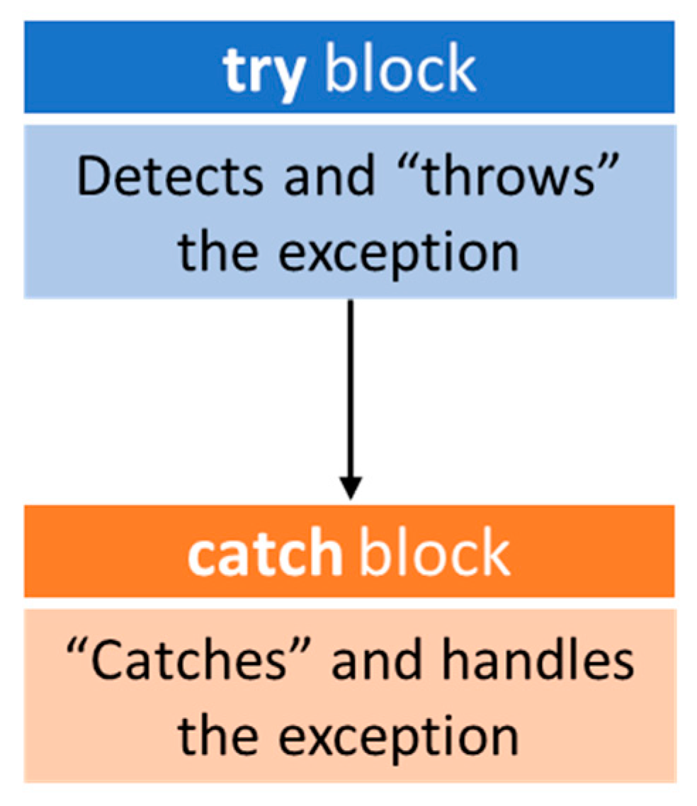
Figure 2.
Comparing “average processing memory” for both the standard calculator and the division by zero calculator.
Figure 2.
Comparing “average processing memory” for both the standard calculator and the division by zero calculator.
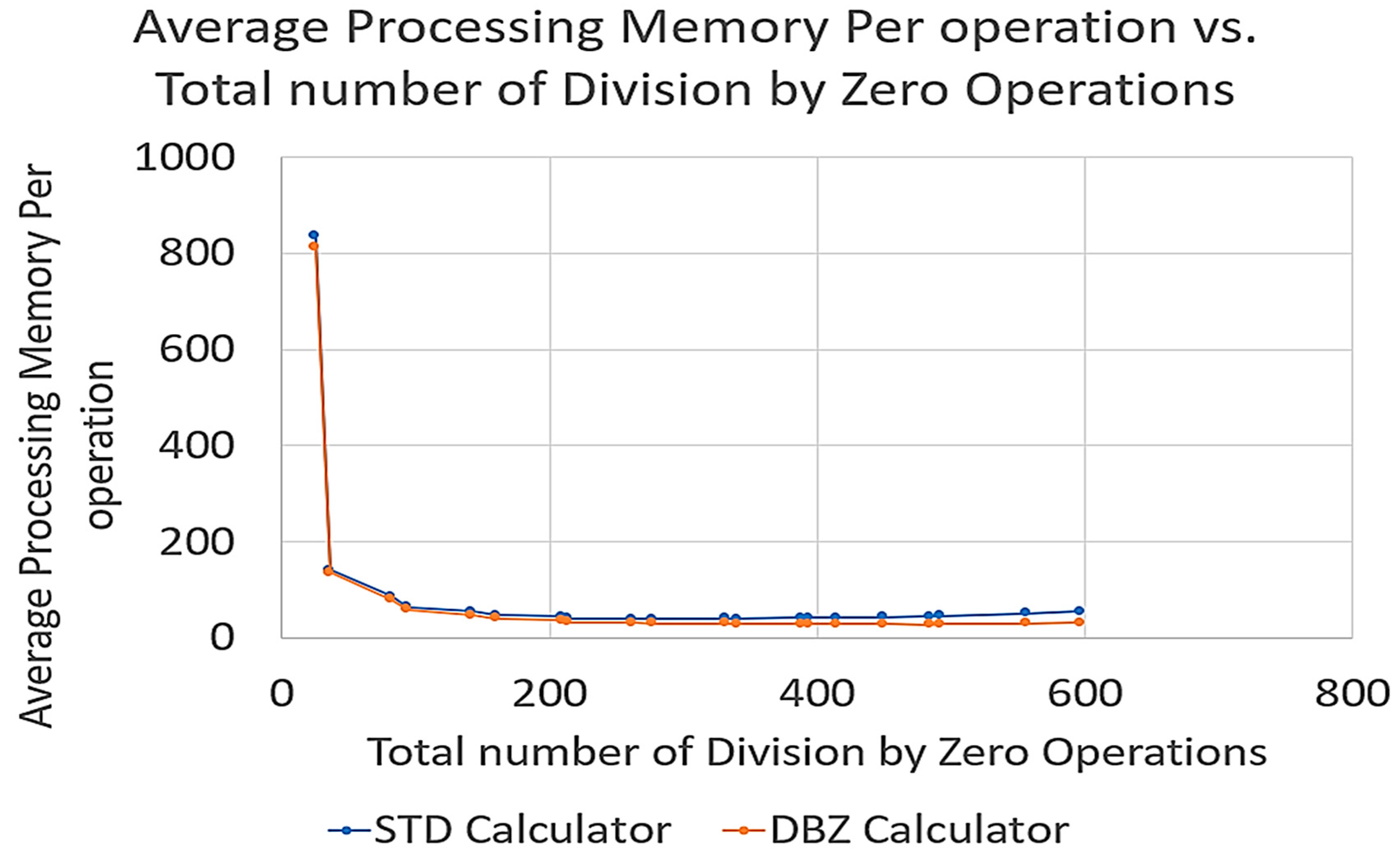
Figure 3.
Total output memory vs. Number of Equations with Division by Zero.
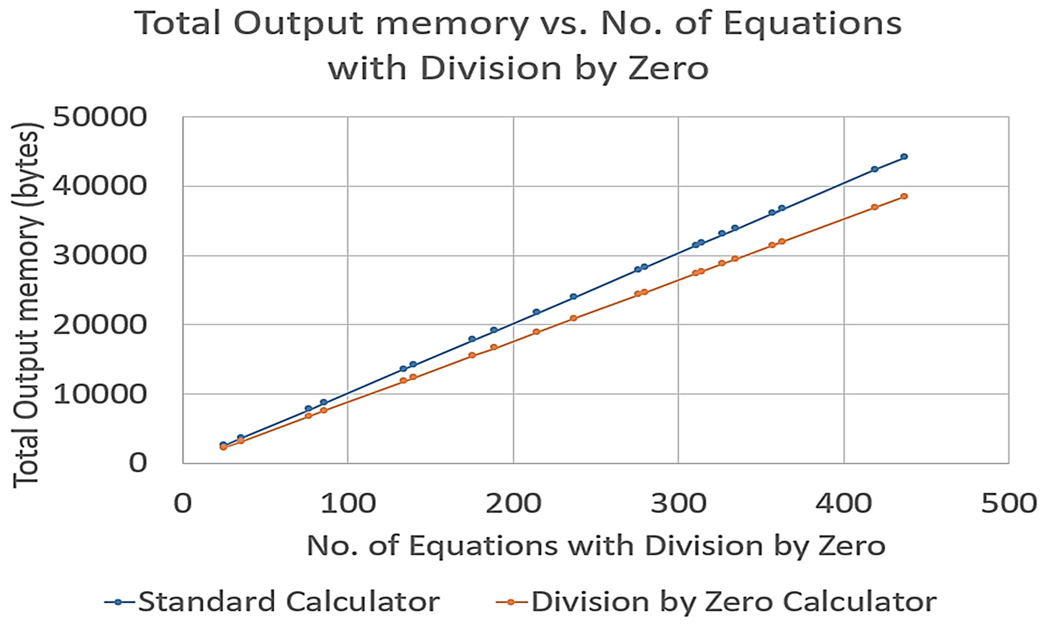
Figure 4.
Comparing Number of operations per unit time against the Total Number of operations for both the standard calculator and the division by zero calculator.
Figure 4.
Comparing Number of operations per unit time against the Total Number of operations for both the standard calculator and the division by zero calculator.
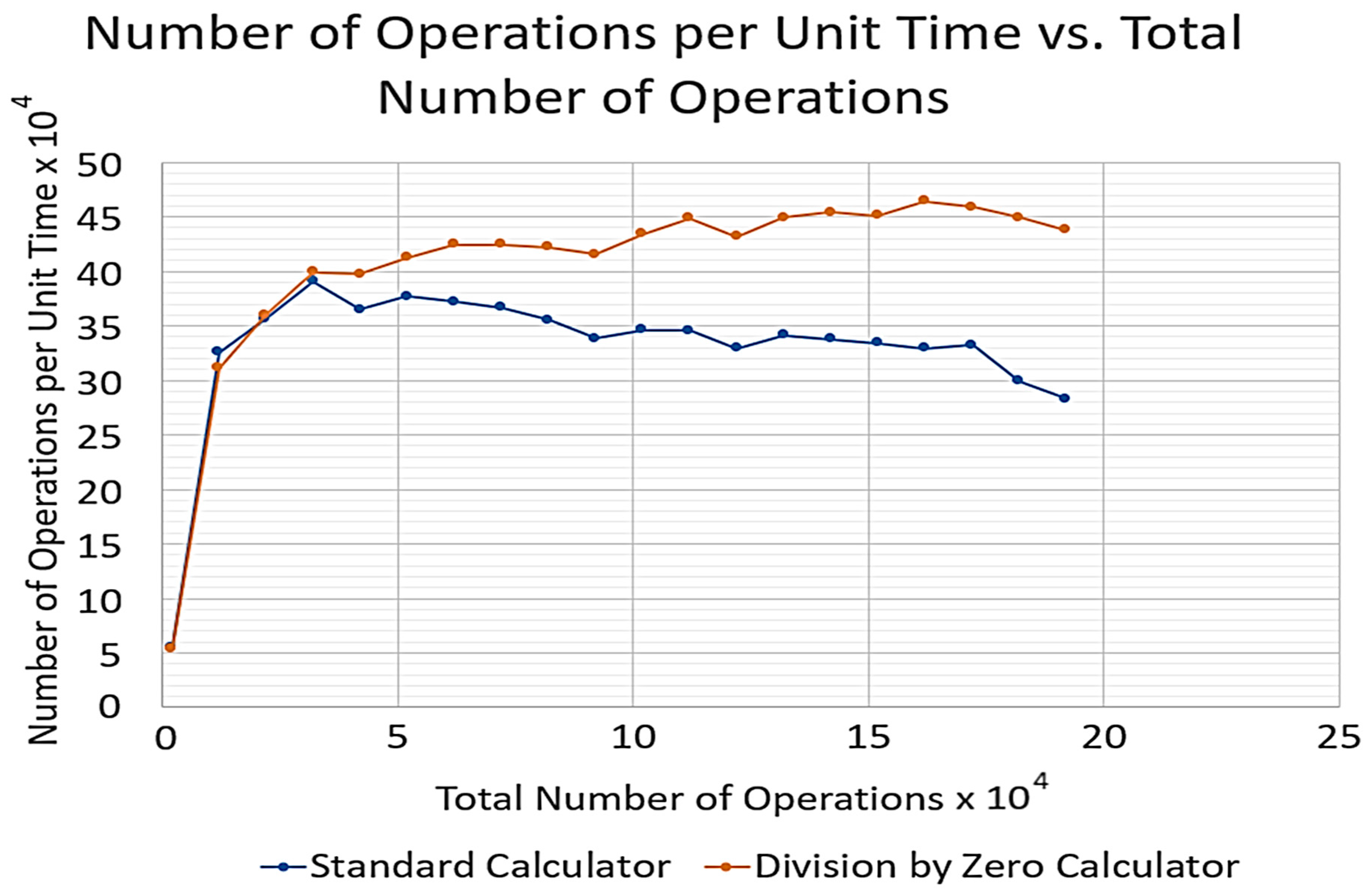
Table 1.
Major results from paper [2].
Table 1.
Major results from paper [2].
 |
Table 2.
Disadvantages of exception handling.
| Disadvantage | Explanation |
|
Exceptions add minute amounts of time to a program’s run time and can cause the program to run slowly if it occurs frequently enough. The key rule of thumb is that exceptions should occur once every 10,000 calls to a computer program [5]. |
|
As the amount of exception handling increase, it’s harder to know which exceptions are more important than others. This could lead to missing a major issue or dismissing an exception that requires immediate attention [5]. |
|
Inserting exception in the middle of coding makes the code cumbersome and difficult to read especially when there are 100s of lines of code. |
Table 3.
infix and associated postfix expressions.
| Infix Expression | Postfix Expression |
Table 4.
Examples of representation of semi-structured complex numbers.
| Semi-structured complex number | Triple format |
Table 5.
Algorithm for semi-structured complex numbers equation generator.
| 1 | User Input: minimum operand value, maximum operand value, equation length L (number of tokens) |
| 2 | If the equation length is less than 3 then set it to 3 |
| 3 | If the equation length (L) is even, then add one to it. (That is, set equation length to L+1) |
| 4 | Create an empty string “Equation” to hold the equation |
| 5 | |
| 6 | For T = 1 to Equation Length do the following: |
| 7 | If T is even then randomly pick an operator from () and add it to the equation string |
| 8 | Else |
| 9 | = Randomly pick integer from range (minimum operand value, maximum operand value) |
| 10 | = Randomly pick integer from range (minimum operand value, maximum operand value) |
| 11 | = Randomly pick integer from range (minimum operand value, maximum operand value) |
| 12 | Add to the Equation string |
| 13 | Return Equation_string |
Table 6.
Examples of equation generated by algorithm in Table 5.
Table 6.
Examples of equation generated by algorithm in Table 5.
| Equation Length L | Equations in Triple format |
Table 7.
Arithmetic Machine STD for a standard semi-structured complex number calculator.
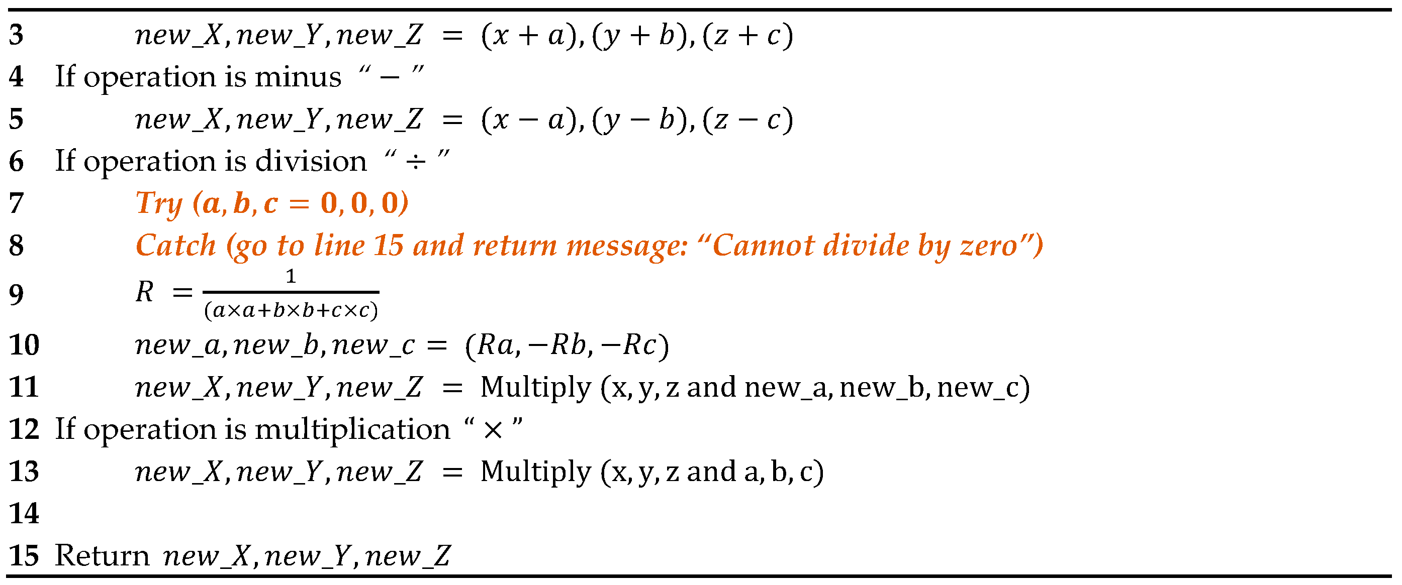 |
Table 8.
“Arithmetic Machine DBZ” for a division by zero calculator.
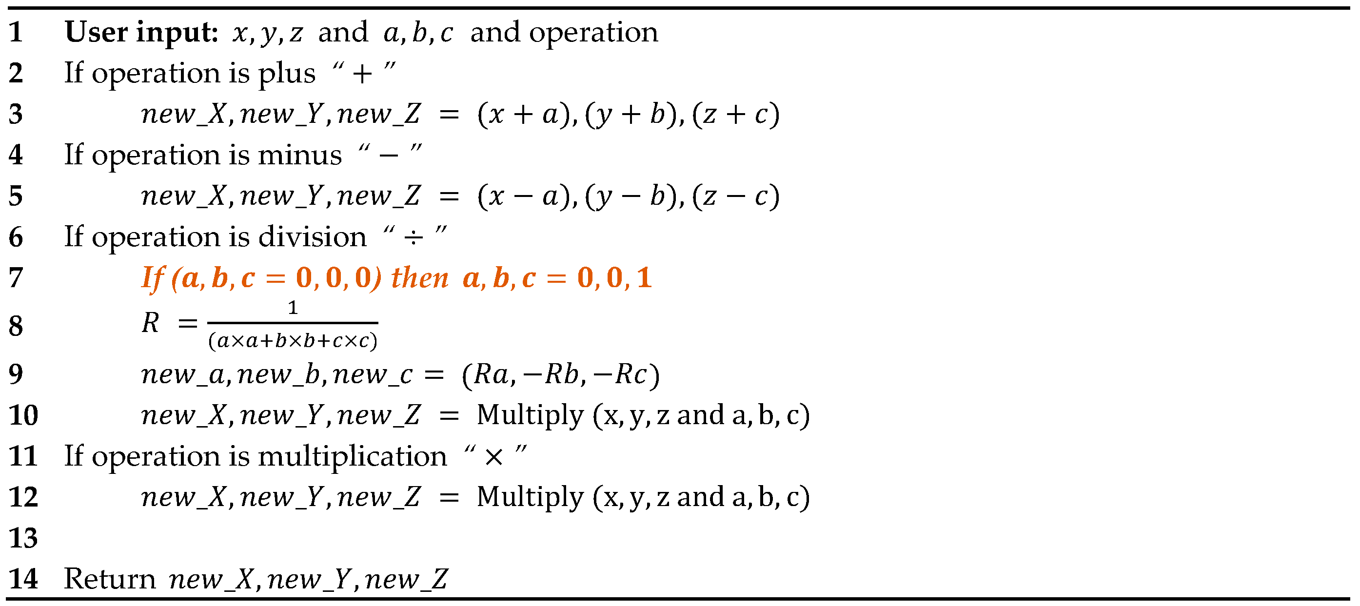 |
Table 9.
General Calculator algorithm.
| 1 | User input: Equation string generated from Equation generator shown inTable 5, Type of Arithmetic Machine: 1 for “Arithmetic Machine STD” and 2 for “Arithmetic Machine DBZ” |
| 2 | Convert Equation string to Postfix Equation string using Infix to Postfix Algorithm shown in Table 14. |
| 3 | Evaluate Postfix Equation string using the Postfix Evaluator Algorithm shown in Table 15 and store in Result string. |
| 4 | |
| 5 | Return Result string |
Table 10.
Space and time complexity measures of efficiency.
| Efficiency Aspect | Measure |
| Space Complexity |
|
|
|
| Time complexity |
|
Table 11.
Efficiency measures of space and time complexity for the standard calculator.
| Characteristics of Equations | Space Complexity | Time Complexity | ||||||||
| Simulation No. | Length of Equation | No. operation per Equation | No. of Equations with DBZ operations |
Total Number of DBZ operations | Total Processing Memory (bytes) |
Average Processing Memory Per operation | Total Output memory (bytes) |
Total Processing Time (microseconds) |
No. of operationsper unit time | No. of Equations successfully computed |
| 1 | 5 | 2 | 25 | 25 | 1628120 | 834.9333 | 2525 | 0.0352 | 55381 | 975 |
| 2 | 25 | 12 | 36 | 36 | 1626846 | 140.6333 | 3636 | 0.0355 | 326020 | 964 |
| 3 | 45 | 22 | 77 | 82 | 1761893 | 86.7671 | 7777 | 0.0570 | 356403 | 923 |
| 4 | 65 | 32 | 86 | 94 | 1874391 | 64.0861 | 8686 | 0.0749 | 390718 | 914 |
| 5 | 85 | 42 | 134 | 142 | 1989516 | 54.6991 | 13534 | 0.0997 | 364648 | 866 |
| 6 | 105 | 52 | 140 | 160 | 2130354 | 47.6376 | 14140 | 0.1186 | 377036 | 860 |
| 7 | 125 | 62 | 176 | 209 | 2256727 | 44.1733 | 17776 | 0.1373 | 372032 | 824 |
| 8 | 145 | 72 | 189 | 214 | 2388216 | 40.8997 | 19089 | 0.1592 | 366720 | 811 |
| 9 | 165 | 82 | 215 | 262 | 2549207 | 39.6024 | 21715 | 0.1811 | 355371 | 785 |
| 10 | 185 | 92 | 237 | 277 | 2775593 | 39.5406 | 23937 | 0.2074 | 338426 | 763 |
| 11 | 205 | 102 | 276 | 331 | 3042633 | 41.2013 | 27876 | 0.2134 | 346129 | 724 |
| 12 | 225 | 112 | 280 | 340 | 3211334 | 39.8231 | 28280 | 0.2333 | 345714 | 720 |
| 13 | 245 | 122 | 311 | 388 | 3563448 | 42.3927 | 31411 | 0.2550 | 329594 | 689 |
| 14 | 265 | 132 | 314 | 394 | 3791536 | 41.8714 | 31714 | 0.2653 | 341300 | 686 |
| 15 | 285 | 142 | 327 | 414 | 4055796 | 42.4397 | 33027 | 0.2831 | 337551 | 673 |
| 16 | 305 | 152 | 335 | 449 | 4393587 | 43.4664 | 33835 | 0.3026 | 333986 | 665 |
| 17 | 325 | 162 | 363 | 484 | 4569098 | 44.2768 | 36663 | 0.3134 | 329304 | 637 |
| 18 | 345 | 172 | 357 | 492 | 4996036 | 45.1737 | 36057 | 0.3330 | 332131 | 643 |
| 19 | 365 | 182 | 419 | 556 | 5405671 | 51.1213 | 42319 | 0.3533 | 299259 | 581 |
| 20 | 385 | 192 | 437 | 597 | 5936380 | 54.9177 | 44137 | 0.3819 | 283015 | 563 |
Table 12.
Efficiency measures of space and time complexity for the “Division by Zero” calculator.
| Characteristics of Equations | Space Complexity | Time Complexity | ||||||||
| Simulation No. | Length of Equation | No. operation per Equation | No. of Equations with DBZ operations |
Total Number of DBZ operations | Total Processing Memory (bytes) |
Average Processing Memory Per operation |
Total Output memory (bytes) |
Total Processing Time (microseconds) |
No. of operations per unit time | No. of Equations successfully computed |
| 1 | 5 | 2 | 25 | 25 | 1627153 | 813.5765 | 2200 | 0.0373 | 53637 | 1000 |
| 2 | 25 | 12 | 36 | 36 | 1626846 | 135.5705 | 3168 | 0.0386 | 311235 | 1000 |
| 3 | 45 | 22 | 77 | 82 | 1761893 | 80.0860 | 6776 | 0.0611 | 360259 | 1000 |
| 4 | 65 | 32 | 86 | 94 | 1874391 | 58.5747 | 7568 | 0.0801 | 399454 | 1000 |
| 5 | 85 | 42 | 134 | 142 | 1989516 | 47.3694 | 11792 | 0.1057 | 397431 | 1000 |
| 6 | 105 | 52 | 140 | 160 | 2130354 | 40.9683 | 12320 | 0.1260 | 412817 | 1000 |
| 7 | 125 | 62 | 176 | 209 | 2256727 | 36.3988 | 15488 | 0.1461 | 424433 | 1000 |
| 8 | 145 | 72 | 189 | 214 | 2388216 | 33.1697 | 16632 | 0.1696 | 424473 | 1000 |
| 9 | 165 | 82 | 215 | 262 | 2549263 | 31.0886 | 18920 | 0.1941 | 422468 | 1000 |
| 10 | 185 | 92 | 237 | 277 | 2775649 | 30.1701 | 20856 | 0.2212 | 415823 | 1000 |
| 11 | 205 | 102 | 276 | 331 | 3042633 | 29.8297 | 24288 | 0.2349 | 434266 | 1000 |
| 12 | 225 | 112 | 280 | 340 | 3211334 | 28.6726 | 24640 | 0.2497 | 448538 | 1000 |
| 13 | 245 | 122 | 311 | 388 | 3563504 | 29.2090 | 27368 | 0.2824 | 432047 | 1000 |
| 14 | 265 | 132 | 314 | 394 | 3791536 | 28.7238 | 27632 | 0.2938 | 449330 | 1000 |
| 15 | 285 | 142 | 327 | 414 | 4055796 | 28.5619 | 28776 | 0.3126 | 454326 | 1000 |
| 16 | 305 | 152 | 335 | 449 | 4394035 | 28.9081 | 29480 | 0.3368 | 451359 | 1000 |
| 17 | 325 | 162 | 363 | 484 | 4569322 | 28.2057 | 31944 | 0.3491 | 464055 | 1000 |
| 18 | 345 | 172 | 357 | 492 | 4996316 | 29.0483 | 31416 | 0.3748 | 458878 | 1000 |
| 19 | 365 | 182 | 419 | 556 | 5406175 | 29.7043 | 36872 | 0.4053 | 449033 | 1000 |
| 20 | 385 | 192 | 437 | 597 | 5936828 | 30.9210 | 38456 | 0.4387 | 437607 | 1000 |
Disclaimer/Publisher’s Note: The statements, opinions and data contained in all publications are solely those of the individual author(s) and contributor(s) and not of MDPI and/or the editor(s). MDPI and/or the editor(s) disclaim responsibility for any injury to people or property resulting from any ideas, methods, instructions or products referred to in the content. |
© 2023 by the authors. Licensee MDPI, Basel, Switzerland. This article is an open access article distributed under the terms and conditions of the Creative Commons Attribution (CC BY) license (https://creativecommons.org/licenses/by/4.0/).
Copyright: This open access article is published under a Creative Commons CC BY 4.0 license, which permit the free download, distribution, and reuse, provided that the author and preprint are cited in any reuse.


