Peptide Hemolytic Activity Analysis using Visual Data Mining of Similarity-based Complex Networks

Kevin Castillo-Mendieta; Guillermin Agüero-Chapin; Nelson Santiago Vispo; Edgar A. Márquez; Yunierkis Perez-Castillo; Stephen J. Barigye; Yovani Marrero-Ponce

doi:10.20944/preprints202303.0322.v1

Preprint

Article

Peptide Hemolytic Activity Analysis using Visual Data Mining of Similarity-based Complex Networks

This version is not peer-reviewed.

Downloads

210

Views

294

Comments

Submitted:

15 March 2023

Posted:

17 March 2023

You are already at the latest version

Abstract

Peptides are promising drug development frameworks thanks to their high target selectivity, tolerability and relatively low production cost. However, despite the fact that several thousand potentially therapeutic peptides reported, only sixty have arrived at the market. This concerning low proportion is partially explained by undesired properties such as peptide-induced hemolytic activity. Hence, we aim to get a better insight into the chemical space of hemolytic peptides using a novel approach based on network science and interactive data mining as an alternative to design more effective peptide drugs with low hemolytic activity. Metadata networks (METNs) were used to characterize and find general patterns associated to hemolytic peptides, whereas Half-Space Proximal Networks (HSPNs), created using five different two-way dissimilarity measures, represented the hemolytic peptide space. Then, using the best candidate HSPNs, we extracted various scaffolds that capture information of almost all the chemical space but avoiding peptide overrepresentation. Such scaffolds can have many applications, such as training accurate ML-based prediction models, constructing one-class multi-query similarity searching models and characterizing the diversity of hemolytic peptides using a manageable set of peptides. Finally, by means of an alignment-free approach, we reported 47 putative hemolytic motifs, which might provide hints about the mechanisms of hemolysis and can also be used as toxic signatures when developing novel peptide-based drugs.

Keywords:

Hemolytic peptide

;

Network science

;

Half-Space Proximal Networks

;

Metadata Networks

;

Visual mining

;

Cluster analysis

;

Motif discovery

;

StarPep toolbox

;

Peptide drug discovery

Subject:

Computer Science and Mathematics - Computer Science

Supplementary Material

supplementary.zip (55.75MB )

1. Introduction

Peptides are relatively small chains of amino acids (AAs) that can be chemically synthesized or purified from living organisms [1]. Our own bodies naturally produce peptides that carry out several critical physiological functions including healing, defense against infections or as chemical messengers [2,3]. Currently, peptides are becoming highly relevant in medical applications as they have shown to exhibit not only promising therapeutic activities such as antimicrobial, antifungal, antiviral, antiparasitic and anticancer but also due to their interesting pharmacological characteristics such as high efficacy, target selectivity and good tolerability [4,5,6]. Peptide drugs were reported to have sales of more than $70 billion in 2019 [7] and in the last decades, they have gained more attention as potential therapeutic drugs than antibodies and small-molecule-based drugs [8,9].

Diseases such as fibrosis, asthma and cancer are treated using peptide-based therapies [2,3]. For instance, the synthetic peptide Leuprolide has been successfully used to treat prostate and breast cancers by acting as an agonist of the gonadotropin-releasing hormone (GnRH) [10]. In addition to Leuprolide, just over 60 therapeutic peptides are commercially available and about 150 are being tested in clinical trials [1,6,11]; however, these numbers are quite low compared with the several thousand potential therapeutic peptides that have been identified [12]. This concerning low proportion of peptide drugs on the market is partially explained by the short half-life, lability during storage, poor oral bioavailability and undesirable toxicity that peptides usually have [2,6,9]. Mainly, peptide-associated hemolysis is perhaps one of the main drawbacks of these potential therapeutic drugs [4] since the products released after the lysis of red blood cells (RBCs) can lead to systemic inflammation and widespread tissue damage [13].

Currently, there are many datasets available containing information about hemolytic peptides. The main databases include: (i) Hemolytik [14], with more than 2000 experimentally validated hemolytic peptides; (ii) Database of Antimicrobial Activity and Structure of Peptides (DBAASP v3) [15], with more than 11321 entries showing information on hemolytic and cytotoxic activities of antimicrobial peptides (AMPs); and (iii) StarPepDB [16] which is a graph-based database that contains 45120 peptides with annotated activities retrieved from multiple sources, from which 2004 are hemolytic peptides [16]. In recent years, some efforts have been made to utilize the information from these databases and predict the hemolytic activity of peptides using machine learning (ML) algorithms [1,2,4,8,9]. However, to our knowledge, no effort has been made to explore the feature space of hemolytic peptides using network science to elucidate the defining characteristics that make certain potential therapeutic peptides hemolytic.

Network science has been previously applied to successfully model many real-world systems [17]. For instance, the ‘small world-model’ introduced by Watts and Strogatz [18] has helped to understand the way different areas of the brain communicate with each other [19]; and more recently, during the Covid-19 pandemic, network science concepts were applied to develop strategies to lower the spread of infection [20,21]. Concerning therapeutic peptides, network science has been recently used to explore the chemical space and build prediction models for tumor-homing peptides [22] and antiparasitic peptides [23], having promising results.

Hence, following the same approach, this report aims to get insight into the chemical space of hemolytic peptides from the StarPepDB using network science and visual (interactive) data mining. Useful information can be retrieved from this strategy, including identifying/delineating the structural diversity among hemolytic peptides, most central and atypical peptides (singletons), the relationship between hemolysis and certain therapeutic activities, and identifying motifs related to hemolytic activity which can be useful when designing therapeutic peptide drugs. Moreover, relatively small subsets of hemolytic peptides can be extracted for further studies. These subsets (called “scaffolds”) have the advantage of representing the whole chemical space of hemolytic peptides but just using a fraction of the nodes of the complex network of hemolytic peptides [24].

Here, we describe for the first time the use of Half-Space Proximal Networks (HSPNs) to represent the chemical space of hemolytic peptides; such networks have been previously used only to explore the antiparasitic peptide space [23]. These networks possess many advantages as they generate highly connected but sparse networks that contain the minimum spanning tree as a sub-graph [25,26]. Moreover, these networks do not strictly need a pairwise similarity threshold (t) between peptides for the construction of informative networks, as is the case of Chemical Space Networks (CSNs) described in other studies. Nevertheless, despite a cutoff value t is not mandatory for HSPNs, it might affect the representativeness of the scaffolds. Hence, we compared HSPNs without a cutoff value (namely t = 0.00) with networks constructed using the same parameters but generated with their optimal similarity cutoff value. Other comparative analyses were also conducted to study the HSPN construction and visualization phase involving the use of distance metrics and centrality measures, respectively, while for extracting a representative subset of hemolytic peptides from the HSPNs, different centrality measures and global and local alignments were also evaluated.

Although, previous studies based on network science have employed the Euclidean distance as the default similarity measure metric; it is suggested that the use of different (dis)similarity measures allows the codification of orthogonal information. Hence it should not be assumed that only one measure is the best suited for calculating the similarity between objects, especially in high dimensional space [27,28,29]. For this reason, we evaluated five different two-way (dis)similarity measures for constructing such HSPNs: (1) Angular Separation, (2) Bhattacharyya, (3) Chebyshev, (4) Euclidean and (5) Soergel. Finally, by using community information from these networks and an alignment-free method for motif discovery, we reported new putative motifs that hallmark hemolytic peptides along with their further enrichment on external datasets to validate their significance.

2. Materials and Methods

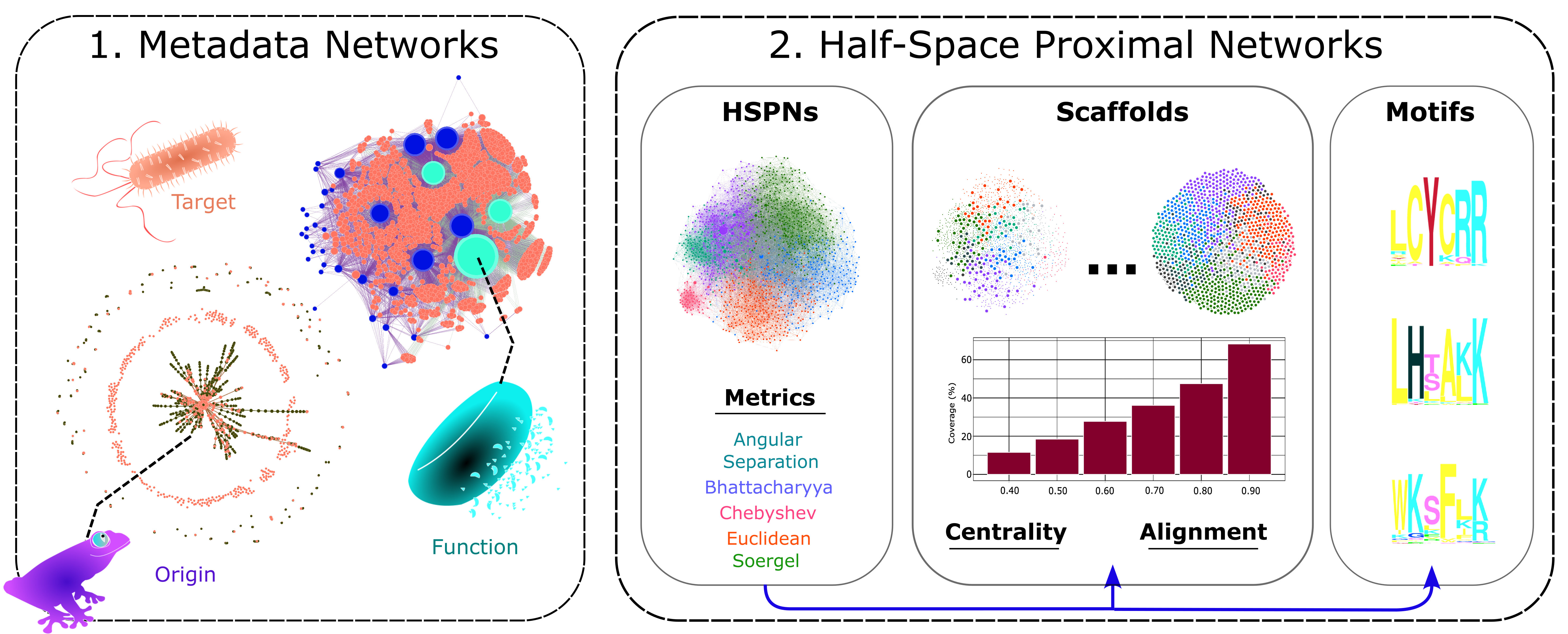
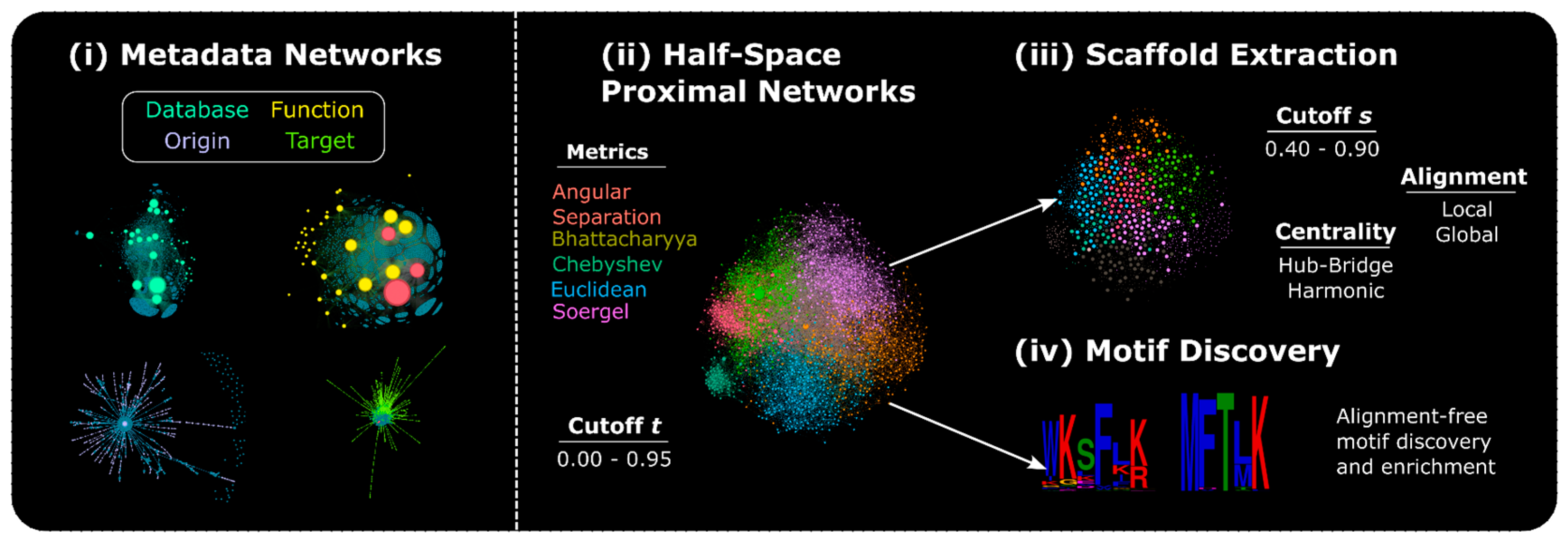
The overall workflow consists of four stages: (i) Metadata network visual mining, (ii) HSPNs generation and analysis, (iii) scaffold extraction and exploration, (iv) motif discovery and enrichment (Figure 1). The first step (Section 2.2.1) involves the generation of metadata networks (METNs) and exploration of critical features related to hemolytic peptides. The second step (section 2.2.2) consists in building HSPNs that represent the chemical space of hemolytic peptides retrieved from StarPepDB. Then the best HSPN candidates were selected based on global network descriptors for further analysis (section 2.2.4). In the third step (section 2.3), representative subsets (scaffolds) from the best HSPN candidates, built up with the optimal t value, and from their respective networks with cutoff t = 0.00 were extracted by using sequence alignment and centrality information from each peptide in the graph. Finally, the last step (section 2.5) consists in proposing new putative hemolytic motifs by using an alignment-free approach and by comparing them with reported hemolytic motifs using benchmark datasets (enrichment analysis) to further select the most representative ones. All the steps of this section were performed using the StarPep toolbox, aided with in-house python scripts and the SeqKit toolkit [30].

2.1 Datasets

The datasets used in this study to construct METNs, HSPNs, generate hemolytic motifs, and subsequently conduct motif enrichment analyses are described in Supplementary Material (file SM1). The usage of each dataset in this report is detailed below.

StarPepDB. It is a graph database embedded in the StarPep toolbox that consists of 45120 peptides with annotated activities retrieved from 40 bioactive databases and other sources [16]. A sub-dataset consisting of 2004 hemolytic peptides was extracted from this database to generate HSPNs, METNs and discover new hemolytic motifs. In addition, the complete StarPepDB was also used in the motif enrichment process to help find the most representative hemolytic motifs.
HemoPI-1. It encompasses 552 experimentally validated highly hemolytic peptides (positive) and 552 random peptides extracted from Swiss-Prot (negative) [8]. This dataset was only used in motif enrichment analysis.
Big-Hemo. It is a non-redundant combination of several datasets that contain either hemolytic or highly hemolytic peptides as positive samples and non-hemolytic or low hemolytic peptides as negative samples. The datasets used to generate the Big-Hemo dataset are HemoPI-2 Main and Validation [8], HemoPI-3 Main and Validation [8], HAPPENN [1], HLPred-Fuse Layer 2 Training and Independent datasets [4] and HemoNet [9]. To construct Big-Hemo, only positive samples labeled as “highly hemolytic” were retrieved from these datasets to handle the problem of lack of agreement and standardization at considering when a peptide is hemolytic or not, and the way of measuring this property, respectively [1,31]. Although HAPPENN dataset contains positive samples not labelled as highly hemolytic, its positive samples were also included in Big-Hemo in order to gain more diversity and a better representation of hemolytic peptides. Thus, this dataset was addressed to evaluate whether our novel motifs are enriched in highly hemolytic peptides, which are more concerning when designing therapeutic peptides. In addition to redundancy removal, peptides containing ‘X’ several times in a sequence and Nphe or Nleu in their sequences were also discarded. The resulting Big-Hemo dataset contains 2196 highly hemolytic peptides. Like HemoPI-1 dataset, Big-Hemo was also used for motif enrichment analysis.

Figure 1. Workflow overview of the experimental procedure. Figure created with Inkscape [32].

2.2 Network Generation and Analysis

2.2.1. Metadata Networks (METNs)

A Metadata Network (METNs) is an unweighted pseudo-bipartite graph defined as

F = (V, E)

, where

E (F)

is the set of edges of the graph and

V (F)

is the set of nodes or vertices which comprises two classes: hemolytic peptides and metadata information (e.g., origin and function of peptides). In these networks, peptide nodes are adjacent to their corresponding metadata nodes. For instance, if a peptide is hemolytic, an edge will connect this peptide node to the hemolytic metadata node. However, METNs are not fully bipartite graphs since in the last ones the nodes belonging to the same class cannot be adjacent [33], whereas METNs can set edges within the metadata class as long as one node is hierarchically related to another. For instance, for the “Function” metadata, “Toxic to mammals” is hierarchically connected to “Hemolytic”, thus an edge connects these two metadata nodes.

StarPep toolbox allows the easy construction of METNs, which help to get insight into the related data associated with the hemolytic peptides. A Database METN, for instance, shows the databases where each hemolytic peptide has been reported by connecting each peptide node to its corresponding database nodes. This information is useful to get an overview of the most populated databases with hemolytic peptides, to analyze peptide redundancy in different databases and also to detect what peptides are uniquely reported in particular dataset, etc. Hence, we created four METNs based on different metadata information: database, function, origin and target. The peptide class of

V (F)

was the set of 2004 hemolytic peptides from StarPepDB.

2.2.2. Half-Space Proximal Networks (HSPNs)

HSPNs, are weighted graphs defined as

G = (V, E)

where

V

(G) represents the set of nodes (hemolytic peptides) and

E (G)

represents the set of edges. The nodes are characterized by vectors whose components are values of sequence-based molecular descriptors (MDs), whereas the edges link nodes in a pairwise manner following the subsequent steps:

A (dis)similarity measure is calculated for each pair of nodes using the vectors of peptide features. Then these values are normalized (min-max normalization). This forms a symmetric similarity matrix $M$ of size $n \times n$ where $n$ represents the number of hemolytic peptides and $M_{i, j}$ represents the similarity score between the nodes $V_{i} (G)$ and $V_{j} (G)$ , being 1 the highest similarity value and 0 the lowest. Then a rule called Half-Space Proximal (HSP) test [26] is applied to construct the HSPN, which is a strongly connected but sparse network [25], that preserves the number of nodes while containing a relatively low number of edges compared to the counterparts, CSNs [25].
Finally, a threshold or cutoff value $t$ can be applied to the weighted edges to further reduce the density of the graph by removing edges whose similarity values are lower than $t$ . This helps to study the topology of the resulting graphs and subsequently find the best representative network of the chemical space occupied by hemolytic peptides. It is worth mentioning that for the construction of HSPNs, using a $t$ value is not mandatory.

HSPNs were constructed as follows. From the 45120 peptides found in StarPepDB [16], 2004 peptides with known hemolytic activity were retrieved using the query option of StarPep toolbox [25]. Redundancy in the peptide sequences was removed using Smith-Waterman local alignment [34] and BLOSUM-62 substitution matrix [35] considering at least 98% sequence identity, resulting in 1647 peptides (SM1.1.3). Then MDs were calculated for each peptide sequence and an unsupervised feature selection was performed, removing near constant peptide features using Shannon entropy (threshold 10%), whereas redundant features were removed using Spearman correlation coefficient (threshold 0.8%). Then all the remaining peptide features were selected for generating the networks. See reference [25] for a detailed description of the peptide feature extraction method.

Regarding the (dis)similarity measures, HSPNs were constructed using Angular Separation (AS), Bhattacharyya (Bh), Chebyshev (Ch), Euclidean (Eu), and Soergel (So) measures. Their formulae and properties are stated in Table 1. We tested several measures since previous studies demonstrated that different distance measures can codify orthogonal information; thus, not necessarily the Euclidean distance might be the best suited for a specific application [27,28].

In addition, to explore the behavior of HSPNs when varying the value of

t

, 11 different cutoffs were applied for each metric: 0.00 and from 0.50 to 0.95 in steps of 0.50, resulting in a total of 55 HSPNs available at SM3 (i.e., 11 networks for each metric). We applied these cutoffs, since a previous study showed that when constructing HSPNs, most of the global parameters barely changed when the similarity cutoff t ranges between 0.00 and 0.45 [23].

Finally, since several combinations will be generated in the following steps, we will use the following notation when referring to a specific network: “cutoff (t)_metric”. For instance, for a network generated with a t = 0.00 using the metric Angular Separation, its corresponding name will be: 0.00_AS.

2.2.3. Network Visualization

For METNs, Betweenness Centrality [36] was calculated and the size of metadata nodes was proportionally projected according to the corresponding centrality value. Database, Function, Origin and Target METNs were visualized by coloring their metadata nodes: aquamarine, yellow, light violet and green, respectively. Metadata nodes related to hemolytic activity (i.e., toxic, toxic to mammals, hemolytic, Red Blood Cells) were colored red. On the other hand, all peptide nodes had the same size and were colored blue-green for all the METNs. Database and Function METNs displayed their most central metadata nodes numbered. Finally, Force Atlas 2 layout algorithm was always used to visualize METNs [37].

For HSPNs, the nodes were clustered using the Louvain method [38], and the Hub-Bridge centrality (HB) measure was calculated for each node. Finally, to better visualize the networks, we colored the nodes according to the cluster they belong to, and the node size was set to be proportional to its HB centrality value using the Bezier interpolator. Finally, we applied the Fruchterman Reingold layout algorithm [39]. The resulting METNs and HSPNs were exported as GraphML files and further visualized with Gephi 0.9.7 [40].

2.2.4. Selection of the best HSPNs

Using Gephi 0.9.7, the following global network parameters were retrieved for each HSPN: number of edges, modularity, density, average clustering coefficient (ACC), number of clusters/communities, singletons GC (nodes disconnected from the giant component), singletons D0 (nodes of degree zero), diameter, average path length, average degree and the probability of

k

(degree distribution). These features were used to study the behavior of the networks and select the best representations for each (dis)similarity measure (five networks in total). The best networks with their optimal cutoff value

t

were then used for scaffold extraction.

2.3 HSPNs Scaffold Extraction and Analysis

This step aims to retrieve representative subsets of the hemolytic peptide space. The five best networks obtained in Section 2.2.4 and the five networks with

t = 0.00

(one for each similarity measure) were used to build the scaffolds. The following steps were applied for each of these networks:

The selected HSPNs were generated again following the steps of Section 2.2.1, but now only the corresponding cutoff value

t

for each network was applied. We also calculated the Harmonic centrality (HC) for each node. After that, we applied the scaffold extraction method (integrated into the StarPep toolbox), which retrieves the most central and unique hemolytic peptides by ranking each peptide in decreasing order regarding their centrality and then redundant sequences were removed as follows: if a pair of sequences have a percentage identity higher than a certain cutoff value

s

1, the least central peptide of the pair will be removed. Finally, the resulting scaffolds of peptide sequences were exported as fasta files. This method generally assures extraction of the most representative peptides from all the centrality ranges but removes sequence redundancy.

Following the same notation for HSPNs, for naming the scaffolds, we inherit the name of the parent network followed by the centrality measure, alignment type, and cutoff

s

value: “cutoff t_metric_centrality_alignment_cutoff s”. For instance, a scaffold extracted from the network 0.00_AS using harmonic centrality, local alignment and a cutoff s = 0.80 would be named as: 0.00_AS_HC_L_0.80.

In this experiment, we varied the type of centrality measure, the sequence alignment type and the cutoff value of percentage identity s. We used Hub-Bridge (HB) or Harmonic centrality (HC), and Needleman-Wunsch global alignment (G) [41] or Smith-Waterman local alignment (L) [34] were used for sequence comparison, both with BLOSUM-62 substitution matrix. Moreover, we tested various cutoff values

s

ranging from 0.40 to 0.90 in steps of 0.10. As a result, for each of the ten selected networks, we generated 24 different scaffolds using the combinations described above. In total 240 scaffolds were obtained (see SM4).

Scaffold Comparison by Metric. For all the scaffolds generated from networks where the cutoff

t = 0.00

, the Jaccard similarity coefficient (JSC) was calculated between scaffold pairs created with the same parameters but differing in their metric. For instance, 0.00_AS_HB_G_0.40 vs. 0.00_Bh_HB_G_0.40. JSC is defined as the number of elements of the intersection of sets A and B divided by the number of elements of the union of those sets [42]. We calculated this distance to assess the similarity between scaffold pairs generated with different parameters.

Scaffold Comparison by Cutoff t, Type of Alignment and Centrality Measure. Using scaffolds constructed from orthogonal metrics (section 2.4.1), we compared the effect of varying the

t

value when generating networks. For this task we calculated the JSC between scaffold pairs created with the same parameters but differing in their

t

value. For instance, 0.00_AS_HB_G_0.40 vs. 0.90_AS_HB_G_0.40. Similarly, the same approach was followed to evaluate the effect of the type of alignment and centrality measure in the representativity of the scaffolds.

All pairwise scaffold comparisons were conducted using SeqKit toolkit to extract peptide IDs and then the relation between sets was obtained using https://bioinformatics.psb.ugent.be/webtools/Venn/.

2.5. Motif Discovery and Enrichment

2.5.1. Motif Discovery

Motif discovery was performed using the alignment-free method STREME (short for Sensitive, Thorough, Rapid Enrichment Motif Elicitation), which finds ungapped motifs enriched in input sequences compared to control sequences providing a statistical significance for each motif [43]. To generate a diversity of potential new hemolytic motifs, we employed the community information of HSPNs with cutoff

t = 0.00

generated with the metrics: Angular Separation, Chebyshev and Euclidean. The following steps were performed for each of the networks:

Using the StarPep toolbox we extracted the sequences of peptides belonging to each cluster (community) and saved them as fasta files. Then these files were used as input sequences for motif discovery. For control sequences, we let the method use shuffled input sequences. Since our peptides contain non-standard AAs, we provided a customized alphabet (SM5.1.1). Motifs ranging from 3 to 6 letters, at least 20% present in the input sequences and with a p-value lower than 0.05 were retrieved.

Similarly, the same steps were applied to retrieve motifs from the file containing 1647 non-redundant hemolytic peptides from StarPepDB. Then, motifs resulting from this process were combined with hemolytic motifs reported in the literature [1,8], and duplicated motifs were removed (see SM5.1.2).

2.5.2. Motif Enrichment

Motif Enrichment was conducted using SEA (Simple Enrichment Analysis) from the MEME suite (https://meme-suite.org/meme/tools/sea). Hemolytic motifs found in section 2.5.1 and motifs reported in the literature [1,8] were employed to assess whether they are enriched in benchmark databases. These motifs were evaluated in HemoPI-1, StarPepDB and Big-Hemo datasets. Sequences labeled as non-hemolytic were used as control sequences in enrichment analysis on HemoPI-1; sequences not having “hemolytic” metadata were used as control when the StarPepDB was used. For enrichment analysis in the Big-Hemo dataset, input sequences were shuffled by the SEA algorithm and used as control sequences. In addition, sequences with length less than three AAs were discarded (SM1.1.3). Finally, those motifs that are statistically significant in all three datasets were kept.

3. Results and Discussion

3.1. Metadata Networks (METNs)

Database METN. Most hemolytic peptides of the StarPepDB come from the SATPdb [12], Hemolytik [14], DBAASP [15], UniProt [44], DRAMP [45] and CyBase [46] databases that are the six most central nodes in Figure 2A. The majority of peptides are shared by SATPdb, Hemolytik, DBAASP and DRAMP, whereas CyBase contains more unique sets of peptides. It might be because CyBase mainly focuses on collecting information about specific types of proteins, cyclic proteins which have shown to possess important advantages such as higher stability and binding affinity compared with linear peptides [47].

In addition, SATPdb has the highest betweenness centrality and node degree value since it is connected to 1817 hemolytic peptides. On the contrary, the databases having the least number of hemolytic peptides are NeuroPep [48], Defensins [49] and Bagel 2 [50] which have node degrees of 4, 2 and 1, respectively. Overall, the Database METN can be helpful when searching for the most important databases regarding peptide hemolytic activity as well as the most unique and most specialized databases.

Function METN. When designing therapeutic drugs, understanding other activities associated with hemolytic peptides can be a good starting point for inferring possible mechanisms of action or chemical characteristics of peptides that might be related not only to certain therapeutic activity but also with hemolysis. A Function METN can be a fast and easy approach to tackle this question by using the StarPep toolbox. Figure 2B shows a Function METN of the 2004 hemolytic peptides reported in the StarPepDB. Evidently, the most central activities are “hemolytic”, “toxic” and “toxic to mammals” since the peptides of study are hemolytic and the aforementioned metadata nodes are hierarchically related (colored red in Figure 2B with centrality ranks: 1, 3 and 5, respectively). However, most of these peptides are also related to antimicrobial activity and hierarchically related metadata: antibacterial, anti-Gram positive, anti-Gram negative, antifungal, etc. In fact, these metadata comprise the nine most central nodes in the Function METN.

Since the main target of antimicrobial peptides (AMPs) is the bacterial cell membrane which is disrupted by several reported modes of action [31], it might be feasible that similar modes of action can also target and disrupt human cells, specifically RBCs. Many studies have proposed that due to the positive charge of many AMPs, they can selectively disrupt negatively charged membranes of bacteria while not affecting the neutral membranes of mammals [51,52]. However, it has been demonstrated that several AMPs (some with high antimicrobial activity) can also disrupt mammalian cells as well, causing hemolysis in RBCs [31,53]. In fact, Function METN shows that 94.46% of the 2004 peptides that comprise the hemolytic space, have both antimicrobial and hemolytic activity.

Origin METN. This type of METN helps to easily identify the origin of hemolytic peptides, whether they are synthetic or isolated from living organisms. Figure 3A shows the complete Origin METN in the dashed box. The central part of the METN was zoomed in and depicted in the center of Figure 3A. Looking at the complete Origin METN three distinctive regions can be observed, an outer ring, a middle ring and a central network. The outer ring represents peptides isolated from living organisms but have not been chemically synthesized. For instance, the peptide StarPep_06954 [54] whose metadata origin node corresponds to only Caenorhabditis elegans. The middle ring represents peptides with nodes of degree zero. This means, peptides that do not have an origin label in the StarPepDB.

On the other hand, the central network shows peptides that have only synthetic origin (the most central blue-green nodes) and peptides isolated from living organisms that have also been chemically synthesized (nodes connected to the central violet metadata node and also connected to radial violet nodes). Radial violet nodes connected in a chain-like way represent hierarchical taxonomic ranks that are related to species from which a particular peptide was obtained. For instance, the subsequent metadata nodes are connected in the following manner Urochordata->Ascidiacea->Pleurogona->Stolidobranchia->Pyuridae->Halocynthia->Halocynthia aurantium. The H. aurantium metadata node is then connected to 6 peptide nodes isolated from that species.

Over half of the hemolytic peptides (1060) are of synthetic construct, whereas the rest are isolated from various organisms. From the top 20 most central origin metadata nodes (synthetic construct not included), half of them belong to the class Amphibia. This is expected because most of the hemolytic peptides in the StarPepDB are antimicrobial (Figure 2B) and a significant part of them have been isolated from frogs and toads since it has been known that they can produce broad-spectrum AMPs in their granular glands in the skin as a defense strategy [55,56,57].

Target METN. An outer ring and a central network can be observed in this METN (Figure 3B). The outer ring of peptides seen in the dashed box are peptides that do not have a metadata node related to a target. This metadata network works in the same fashion as the Origin METN, where chain-like nodes represent the hierarchical taxonomic ranks, but instead of representing the origin of the peptide, it displays the target of the peptide i.e., the species/cell type in which a certain peptide activity has been evaluated. Evidently, the main target is human erythrocytes (colored red in Figure 3B) since we are exploring the hemolytic peptide space. Other central targets include Escherichia coli, Staphylococcus aureus, Pseudomonas aeruginosa, Bacillus subtilis and Candida albicans. They are among the six most central metadata nodes in this METN. It shows that several of the hemolytic peptides have been evaluated as potential AMPs in important human pathogens such as P. aeruginosa which has become a real concern in hospital-acquired infections due to drug-resistance appearance [58].

GraphML files of METNs and the descriptor information from each node are available at SM2.

3.2. Half-Space Proximal Networks (HSPNs)

The properties of the HSPNs were studied based on their global network parameters consisting of the number of edges, modularity, density, average clustering coefficient (ACC), number of communities and singletons, among others. Such statistics can provide a good picture of the topology of the graphs and help selecting networks with the cutoff t that better projects the chemical space of hemolytic peptides.

Our results are consistent with another study that showed that there was little change in the global network parameters when networks are created within the cutoff t range 0.00 – 0.45 [23]. This is because of the highly low number of edges that are removed within this range. In fact, on average, the number of removed edges at

t = 0.50

correspond to the 1.9% of the initial edges when

t = 0.00

(See SM3.6).

Moreover, it can be observed that networks generated by different metric measures address differently the similarity between peptides (Figure 4). Based on their behavior, the networks used in this study can be roughly grouped into three classes: Class I: Angular Separation; Class II: Bhattacharyya, Euclidean and Soergel; and Class III: Chebyshev. The influence of the metric measure in the global parameters of the networks is provided below. All global network parameters calculated for each metric are provided in SM3.

Modularity. This is a measure of the network connectivity which indirectly represents how well-defined communities are in the graph and is associated with the number of communities. Graphs generated with Angular Separation (AS) initially possess higher modularity values compared to the other metrics; however, the modularity keeps relatively low at higher t values (0.550 at t = 0.95) whereas the other four metrics increase their modularity to values near 1. On the other hand, Chebyshev (Ch) networks show the lowest modularity at low cutoff values, but then it increases to high values comparable with Soergel (So), Euclidean (Eu) and Bhattacharyya (Bh). So- and Eu-derived networks have a quite similar behavior in the whole range of t values, whereas Bh networks initially behave similar to Eu and So networks, but then diverge at t = 0.70 (Figure 4A). An adequate selection of modularity is important since highly sparse networks with an elevated number of communities would not provide useful information as several resulting communities would be just artifacts.

Density. It shows the ratio between the edges present in the network and the maximum number of possible edges. Similarity networks have been shown to have an inversely proportional relationship between similarity threshold (t) and density [25,60]. The same pattern is observed for all metrics, but with some notable variations. Here, we can identify three behaviors according to the three class of metrics. AS networks have the highest density in the entire range of t, whereas Class II metrics (i.e., Bh, Eu, and So) have the lowest density until t = 0.70. On the other hand, Ch networks not only have an intermediate initial density but also show the biggest variation of density along the whole range of t (Figure 4C). In order to select adequate networks, we should choose graphs that are neither too dense nor too sparce since the former would hamper retrieval of useful information whereas the latter would lose information [61]. Density values below 0.20 are desired as they allow to properly understand the network while preserving high modularity. Particularly, HSPNs are suited because they have the intrinsic characteristic of showing low densities. In fact, the highest density value in this study corresponds to 0.020 (0.00_AS network).

Average Clustering Coefficient (ACC). This measures the connectivity of the network and it has been previously studied on molecular similarity networks varying the similarity cutoff t. One study showed that the ACC maximum peak correlates with the best clustering outcome and is a good indicator for finding the appropriate value of t [60]. In our study, three behaviors related to the metric class can be observed again. AS networks have the highest ACCs in the whole range of t with its local maximum at t = 0.95. On the other hand, Ch networks start with very low ACCs and get increased at t = 0.65 reaching its maximum peak at t = 0.90. Finally, Class II metrics have the lowest ACCs in the entire range of t with their maximum peaks at 0.70 (Eu), 0.80 (So) and 0.85 (Bh) (Figure 4E).

Communities and singletons. The number of communities determined with the Louvain method, the number of singletons D0 (nodes of degree zero) and the number of singletons GC (nodes disconnected from the giant component) were calculated to select the networks with the most reasonable values of these parameters. When t = 0.00, HSPNs have the minimum spanning tree as a subgraph, this implies that at this t value all nodes are connected. In other words, no singletons D0 nor singletons GC are found. Regarding the number of communities at t = 0.00, all metric networks showed similar values (on average 8 communities). At higher t values, the number of communities and singletons D0 increase dramatically for all the metric networks, except for AS networks (Figure 4B–D). This is expected as more edges are removed, more nodes are isolated, and now singletons are counted within the communities. Hence, an appropriate t value should be selected that comprises an equilibrium between singletons (atypical peptides) and communities that reflect a real chemical relationship.

Other global network parameters were also calculated to characterize the networks, such as the diameter of the graph (Figure 4F), the average path length (APL) and average degree (See SM3.6). In order to find the best t value for each metric network, we should look for a compromise between the best parameter value for each descriptor i.e., networks with low density, with neither too many clusters (< 20) nor too many singletons (~15-30), retaining high ACC and high modularity. The global descriptors of the selected networks with their best cutoff value t and their respective networks constructed with t = 0.00 (10 networks in total) are shown in Table 2.

Finally, we calculated the probability of k (also known as the degree distribution) for each of the selected networks (Figure 5). Overall, all networks show a right-skewed bell-shaped distribution with high probability of intermediate node degrees. Evidently, plots on the left (t = 00) show a probability of zero for singletons (k = 0) whereas plots on the right (best value t) tend to have a higher probability when k = 0. In addition, plots with the best t value have smaller maximum degrees (as well as the average degree) compared with same-metric networks at t = 0.00. Thus, when comparing networks with the same metric but varying the cutoff value (t = 0.00 vs. best cutoff t), it seems both retain a similar degree distribution. However, when comparing networks with different metrics we can get marked differences. AS networks tend to have a wider distribution range and a higher average degree whereas Ch networks show intermediate values, and networks constructed with Class II metrics show a similar distribution shape among them and have the lowest distribution ranges and average degrees of all metrics. Figure 6 shows the graphical representation of the 10 selected HSPNs.

3.3. HSPNs Scaffolds

A total of 240 scaffolds were extracted from the 10 HSPNs selected in section 3.2 (SM4.1). To better understand the effect of the centrality measure, type of alignment and cutoff value s when constructing the scaffolds, several pairwise similarity comparisons between scaffolds were carried out using the JSC between sets of hemolytic peptides [42].

Metric Comparison. We compared the type of metric measure used to build the parental networks of the scaffolds. For this comparison, scaffolds (t = 0.00) built with the same combinations of centrality, alignment, and cutoff s but with different metrics were evaluated (SM4.3.1). Each pair of scaffolds is represented as a point in Figure 7. In all plots of Figure 7 when s ≥ 0.60, all scaffold pairs constructed with Class II metrics (i.e., Bh, Eu, So) show the highest similarity percentage compared with the pairs from other combination of metrics. Moreover, scaffold pairs in which one of them is extracted by the AS metric show the smallest similarity percentage at almost any cutoff value s. On the contrary, scaffolds selected with Ch metric have an intermediate similarity percentage when compared with scaffolds extracted by other metrics. These results agree with section 3.2 which showed that the five metrics tend to have three types of behavior (three classes of metrics). The density (Figure 4C) and the degree distribution (Figure 5) of the networks with different metrics are the global descriptors most correlated with the results from the percentage similarity among scaffolds. Thus, it is possible to reduce the number of highly-similar scaffolds by using only those HSPNs with the metrics that mostly differ in the aforementioned global network parameters. In this case, Class II metrics: Bh, Eu, and So are the metric measures with the most similar behavior since they produce similar networks and scaffolds. Therefore, it was decided to conduct the following analyses using only one of the metrics of Class II: Euclidean. This metric was chosen since it is the default metric used in other studies [22,23], and it would be advantageous to compare its performance with the other metrics not previously used in this type of study. Overall, this step allowed us to reduce the redundancy in the scaffold representativity from 240 to 144 scaffolds (SM4.2).

Cutoff Comparison. A cutoff value t is not mandatory when constructing HSPNs since at t = 0.00, these networks already have low densities under 0.20. However, the topology, characterized by global network features, tends to vary when varying t as was demonstrated in section 3.2. Thus, it is important to evaluate the effect of selecting a cutoff value (or not) when constructing representative scaffolds of the chemical space. The JSC was calculated between pairs of scaffolds extracted by using the same metric but at different cutoff values (t = 0.00 vs. best t value), see SM4.3.2 (Figure 8).

A marked difference was observed when these scaffold pairs were constructed with different types of centralities. Scaffolds constructed with HB centrality (Figure 8A,B) tend to have more unique peptides at low s values and the number of common peptides between scaffold pairs tend to increase when s increases. A similar pattern was observed in Figure 7. However, when the same scaffolds are constructed replacing HB centrality with HC centrality all scaffold pairs tend to share more than 89.50% of peptides regardless of the value of s (SM4.3.2.2) (Figure 8C,D). Furthermore, the same patterns are preserved when any alignment type is applied. Hence, when generating scaffolds using HC centrality, it is unnecessary to first find the best t value for the parental networks since similar scaffolds will be obtained using networks with t = 0.00.

Alignment Comparison. A clear pattern can be observed when extracting scaffold either using global or local alignment (Figure 7 and Figure 8). In general, local alignment tends to discriminate more strongly at low s values than global alignments. Hence, scaffold pairs extracted with local alignment at such low s values have a lower similarity percentage than the analogue scaffold pairs extracted using global alignment.

In addition, when comparing the similarity percentage of scaffold pairs extracted using the same parameters but differing the alignment type, the same behavior was observed independently of the metric, type of centrality or the t value used, see Figure 9. Scaffold pairs differing only in their alignment type tend to have a low percentage of similarity at low s values, which might indicate that these methods capture the similarity between peptides differently. However, when analyzing the proportion of unique peptides between these scaffold pairs, it is clear that scaffolds extracted using local alignment are practically a subset of scaffolds extracted when using global alignment. In fact, the average number of unique sequences in local scaffolds when comparing them with their global counterparts at any cutoff s is 16.19 (SM4.3.3). An example is provided for the scaffold pairs: 0.00_AS_HB_G_0.40 and 0.00_AS_HB_L_0.40 (Figure 10).

Centrality Comparison. Pairwise comparisons of the scaffolds constructed using the same parameter but changing the centrality measure show a trend like the pairwise comparisons presented before (SM4.3.4). This implies that the type of centrality used to extract the scaffold will affect in the sequences that are removed/retained, especially at low s values.

On the other hand, when comparing centrality measures, JSC between scaffold pairs extracted from networks with best t value tend to be higher than JSC from scaffold pairs from networks with t = 0.00. This pattern is clearer at low s values (Figure 11).

All scaffolds presented in this section can be used in many applications. For instance, they can be used as training datasets for both ML-based and Multi-Query Similarity Searching (MQSS) prediction models of hemolytic peptides. The advantage of using these datasets is that they store information of central and important peptides as well as outliers or atypical hemolytic peptides while avoiding overrepresentation of certain peptide classes (sampling bias). Each scaffold bears a unique type and amount of information of the hemolytic peptide space and one scaffold can be more suitable than another depending on the scaffold’s use. Scaffolds extracted at low cutoff s values tend to cover fewer peptides of the original space, whereas higher s values capture more information of the space but peptide overrepresentation might be present. Even scaffolds with s = 0.90 have on average 71.48% coverage of the total hemolytic peptide space, which is still an adequate equilibrium between coverage and amount of information. Figure 12 depicts an example of the scaffold coverage when varying the cutoff s.

3.4. Hemolytic Motif Discovery and Enrichment

Motif Discovery. Peptides from each community were used as input sequences to uncover new hemolytic motifs within the communities’ diversity by means of STREME, an alignment-free method [43]. Table 3 shows a sample of the 42 new motifs discovered using clusters of HSPNs (t = 0.00) created with different metrics. 12 motifs were found from 6 clusters of the network 0.00_AS, 14 motifs were discovered from 4 clusters of the network 0.00_Ch and 16 motifs from 5 clusters were discovered using the network 0.00_Eu. The three metrics commonly detected only 4 motifs: GLP, MFTKL, ERBADE and VCTRN. It is worth mentioning that several other motifs were similar but not identical such as: GLP/GLPV or VGGTCN/GGTCN. In addition, 15 motifs were discovered not considering the community diversity by using all 1647 hemolytic peptides as input sequences. All these motifs were grouped as HSPNs motifs. After removing duplicated motifs, 50 HSPNs motifs were discovered (SM5.1.2).

Two previous reports on ML models for predicting hemolytic activity of peptides have also reported hemolytic motifs, namely: HemoPI [8] and HAPPENN [1]. HemoPI reported 21 motifs extracted using MERCI software that were enriched in positive sequences from HemoPI-1 and HemoPI-2 datasets, whereas HAPPENN motifs resulted by looking for the 20-top motifs found exclusively in the positive dataset of HAPPENN. No HSPN-derived motifs were found among the reported ones. To generate a unique list of non-redundant hemolytic motifs, HSPNs motifs were combined with the previously reported ones resulting in 91 putative motifs. Then similar motifs were combined into consensus motifs resulting in 57 non-redundant motifs (SM5.1.2 and SM5.1.3).

Motif Enrichment. To identify and validate the most representative hemolytic motifs and remove some artifacts from the 57 potential hemolytic motifs, we conducted enrichment analyses using SEA method on three different datasets: HemoPI-1, StarPepDB and Big-Hemo (SM5.2). Motifs not reported as significant in at least one dataset were removed. The resulting 47 hemolytic motifs sorted by the average enrichment ratio of all datasets are presented below (newly discovered motifs by HSPNs are shown in red):

MFTLK, ALKAIS, GTCN, WKSFJK, VCGETC, WKK, AKKAL, GETCV, CYCR, LKKL, CVCV, ISWIK, RFC, LHTA[KL], FLHSAK, CSW, LWKT, FLGTI, GAVLKV,PGC, KKILG, KITK, KHI, LGKL, KWK, VNWK, K[GT]AGK, VCT, ALW, SWP, HIF,LLKK, [VI]LDTJ, CRR, KLL, JGKL, FKK, GAIA, VLK, GLP, PKIF, GKEV, GTIS, AAAK, GCS, IAS, MAL (Table 4).

These motifs might be involved in the mechanisms of action of hemolytic peptides as well as antimicrobial activity but further studies are needed to corroborate this assumption. Another possible use of these motifs can be as a toxic signature, where proteins containing some of these motifs could be attributed to a relatively high hemolytic activity in comparison with proteins with few or none hemolytic motifs. Table 5 shows an example of three pairs of peptides whose hemolytic activity is related to the number of hemolytic motifs present in their sequences.

4. Conclusions

Positive endpoints are commonly evaluated in peptides to better understand a specific therapeutic activity; however, getting insight into negative endpoints such as hemolysis should be equally important. In this study, the exploration of the chemical space of hemolytic peptides through a synergic combination of network science and interactive data mining resulted in an easy and feasible way to get more insight into the features that characterize this type of peptides. For instance, the hemolytic activity was almost exclusively associated with AMPs, from which the majority are of synthetic construct or isolated from frogs and toads. Moreover, scaffolds and motifs extracted from the hemolytic peptide space can aid future studies related to description of hemolytic peptide families, assessment of the mechanisms of hemolysis, and training ML- and MQSS-based prediction models. The main asset of this approach is that it can easily be extrapolated to many other peptide types such as AMPs, industrial enzymes, therapeutic hormones, etc.

Supplementary Materials

The following supporting information can be downloaded at: www.mdpi.com/xxx/s1. SM1 – Datasets used in the study labelled as StarPepDB, Big-Hemo and HemoPI-1. SM2 – Additional data relative to the METNs of hemolytic peptides (GraphML files and Node properties). SM3 – HSPNs projection with different metrics at varying the value of

t

, (GraphML files), and selection of the optimal similarity cutoff

t

(excel file). SM4 – Scaffolds extracted from the HSPNs and pairwise comparison for their selection. SM5 – Motif discovery analyses and resulting hemolysis-related motifs.

Author Contributions

K.C.-M. was involved in all experiments and writing of the manuscript. G.A.-C. and Y.M.-P. worked mainly on the conceptualization, formal analysis, supervision, validation, writing and reviewing of the manuscript. E.A.-M. and Y.P.-C. worked/supervised data curation and analyses of METNs and HSPNs representing the hemolytic peptide space. S.J.-B. and N.S.-V. were responsible for the scaffold extraction and selection as well as the new hemolysis-related motifs discovery. All authors have read and agreed to the published version of the manuscript.

Funding

Declared none.

Institutional Review Board Statement

Not applicable.

Informed Consent Statement

Not applicable.

Data Availability Statement

The starPep toolbox software and the respective user manual, are freely available online at http://mobiosd-hub.com/starpep. The data supporting reported results can be found at: www.mdpi.com/xxx/s1

Acknowledgments

Y.M.-P. thanks to the program “Profesor invitado” for a post-doctoral fellowship to work at Valencia University in 2020, to the support from Collaboration Grant 2021-22 (Project ID16897) and Med Grant 2023 (Project ID16905). G.A.-C. and A.A. were supported by national funds through FCT - Foundation for Science and Technology within the scope of UIDB/04423/2020 and UIDP/04423/2020.

Conflicts of Interest

The authors declare no conflict of interest.

References

Timmons, P.B.; Hewage, C.M. HAPPENN Is a Novel Tool for Hemolytic Activity Prediction for Therapeutic Peptides Which Employs Neural Networks. Sci Rep 2020, 10, 10869. [Google Scholar] [CrossRef] [PubMed]
Win, T.S.; Malik, A.A.; Prachayasittikul, V.; S Wikberg, J.E.; Nantasenamat, C.; Shoombuatong, W. HemoPred: A Web Server for Predicting the Hemolytic Activity of Peptides. Future Medicinal Chemistry 2017, 9, 275–291. [Google Scholar] [CrossRef] [PubMed]
Xiao, Y.-F.; Jie, M.-M.; Li, B.-S.; Hu, C.-J.; Xie, R.; Tang, B.; Yang, S.-M. Peptide-Based Treatment: A Promising Cancer Therapy. Journal of Immunology Research 2015, 2015, e761820. [Google Scholar] [CrossRef] [PubMed]
Hasan, M.M.; Schaduangrat, N.; Basith, S.; Lee, G.; Shoombuatong, W.; Manavalan, B. HLPpred-Fuse: Improved and Robust Prediction of Hemolytic Peptide and Its Activity by Fusing Multiple Feature Representation. Bioinformatics 2020, 36, 3350–3356. [Google Scholar] [CrossRef] [PubMed]
Kumar, V.; Kumar, R.; Agrawal, P.; Patiyal, S.; Raghava, G.P.S. A Method for Predicting Hemolytic Potency of Chemically Modified Peptides From Its Structure. Front Pharmacol 2020, 11, 54. [Google Scholar] [CrossRef] [PubMed]
Plisson, F.; Ramírez-Sánchez, O.; Martínez-Hernández, C. Machine Learning-Guided Discovery and Design of Non-Hemolytic Peptides. Sci Rep 2020, 10, 16581. [Google Scholar] [CrossRef] [PubMed]
Wang, L.; Wang, N.; Zhang, W.; Cheng, X.; Yan, Z.; Shao, G.; Wang, X.; Wang, R.; Fu, C. Therapeutic Peptides: Current Applications and Future Directions. Sig Transduct Target Ther 2022, 7, 1–27. [Google Scholar] [CrossRef] [PubMed]
Chaudhary, K.; Kumar, R.; Singh, S.; Tuknait, A.; Gautam, A.; Mathur, D.; Anand, P.; Varshney, G.C.; Raghava, G.P.S. A Web Server and Mobile App for Computing Hemolytic Potency of Peptides. Sci Rep 2016, 6, 22843. [Google Scholar] [CrossRef]
Yaseen, A.; Gull, S.; Akhtar, N.; Amin, I.; Minhas, F. HemoNet: Predicting Hemolytic Activity of Peptides with Integrated Feature Learning. J Bioinform Comput Biol 2021, 19, 2150021. [Google Scholar] [CrossRef]
Wilson, A.C.; Vadakkadath Meethal, S.; Bowen, R.L.; Atwood, C.S. Leuprolide Acetate: A Drug of Diverse Clinical Applications. Expert Opinion on Investigational Drugs 2007, 16, 1851–1863. [Google Scholar] [CrossRef]
Lee, A.C.-L.; Harris, J.L.; Khanna, K.K.; Hong, J.-H. A Comprehensive Review on Current Advances in Peptide Drug Development and Design. International Journal of Molecular Sciences 2019, 20, 2383. [Google Scholar] [CrossRef] [PubMed]
Singh, S.; Chaudhary, K.; Dhanda, S.K.; Bhalla, S.; Usmani, S.S.; Gautam, A.; Tuknait, A.; Agrawal, P.; Mathur, D.; Raghava, G.P.S. SATPdb: A Database of Structurally Annotated Therapeutic Peptides. Nucleic Acids Research 2016, 44, D1119–D1126. [Google Scholar] [CrossRef] [PubMed]
Van Avondt, K.; Nur, E.; Zeerleder, S. Mechanisms of Haemolysis-Induced Kidney Injury. Nat Rev Nephrol 2019, 15, 671–692. [Google Scholar] [CrossRef] [PubMed]
Gautam, A.; Chaudhary, K.; Singh, S.; Joshi, A.; Anand, P.; Tuknait, A.; Mathur, D.; Varshney, G.C.; Raghava, G.P.S. Hemolytik: A Database of Experimentally Determined Hemolytic and Non-Hemolytic Peptides. Nucleic Acids Research 2014, 42, D444–D449. [Google Scholar] [CrossRef] [PubMed]
Pirtskhalava, M.; Amstrong, A.A.; Grigolava, M.; Chubinidze, M.; Alimbarashvili, E.; Vishnepolsky, B.; Gabrielian, A.; Rosenthal, A.; Hurt, D.E.; Tartakovsky, M. DBAASP v3: Database of Antimicrobial/Cytotoxic Activity and Structure of Peptides as a Resource for Development of New Therapeutics. Nucleic Acids Research 2021, 49, D288–D297. [Google Scholar] [CrossRef] [PubMed]
Aguilera-Mendoza, L.; Marrero-Ponce, Y.; Beltran, J.A.; Tellez Ibarra, R.; Guillen-Ramirez, H.A.; Brizuela, C.A. Graph-Based Data Integration from Bioactive Peptide Databases of Pharmaceutical Interest: Toward an Organized Collection Enabling Visual Network Analysis. Bioinformatics 2019, 35, 4739–4747. [Google Scholar] [CrossRef] [PubMed]
Vespignani, A. Twenty Years of Network Science. Nature 2018, 558, 528–529. [Google Scholar] [CrossRef]
Watts, D.J.; Strogatz, S.H. Collective Dynamics of ‘Small-World’ Networks. Nature 1998, 393, 440–442. [Google Scholar] [CrossRef] [PubMed]
Sporns, O.; Chialvo, D.R.; Kaiser, M.; Hilgetag, C.C. Organization, Development and Function of Complex Brain Networks. Trends in Cognitive Sciences 2004, 8, 418–425. [Google Scholar] [CrossRef]
Roy, S.; Cherevko, A.; Chakraborty, S.; Ghosh, N.; Ghosh, P. Leveraging Network Science for Social Distancing to Curb Pandemic Spread. IEEE Access 2021, 9, 26196–26207. [Google Scholar] [CrossRef]
Roy, S.; Biswas, P.; Ghosh, P. Effectiveness of Network Interdiction Strategies to Limit Contagion During a Pandemic. IEEE Access 2021, 9, 95862–95871. [Google Scholar] [CrossRef]
Romero, M.; Marrero-Ponce, Y.; Rodríguez, H.; Agüero-Chapin, G.; Antunes, A.; Aguilera-Mendoza, L.; Martinez-Rios, F. A Novel Network Science and Similarity-Searching-Based Approach for Discovering Potential Tumor-Homing Peptides from Antimicrobials. Antibiotics 2022, 11, 401. [Google Scholar] [CrossRef]
Ayala-Ruano, S.; Marrero-Ponce, Y.; Aguilera-Mendoza, L.; Pérez, N.; Agüero-Chapin, G.; Antunes, A.; Aguilar, A.C. Network Science and Group Fusion Similarity-Based Searching to Explore the Chemical Space of Antiparasitic Peptides. ACS Omega 2022, 7, 46012–46036. [Google Scholar] [CrossRef] [PubMed]
Agüero-Chapin, G.; Galpert-Cañizares, D.; Domínguez-Pérez, D.; Marrero-Ponce, Y.; Pérez-Machado, G.; Teijeira, M.; Antunes, A. Emerging Computational Approaches for Antimicrobial Peptide Discovery. Antibiotics 2022, 11, 936. [Google Scholar] [CrossRef]
Aguilera-Mendoza, L.; Marrero-Ponce, Y.; García-Jacas, C.R.; Chavez, E.; Beltran, J.A.; Guillen-Ramirez, H.A.; Brizuela, C.A. Automatic Construction of Molecular Similarity Networks for Visual Graph Mining in Chemical Space of Bioactive Peptides: An Unsupervised Learning Approach. Sci Rep 2020, 10, 18074. [Google Scholar] [CrossRef]
Chavez, E.; Dobrev, S.; Kranakis, E.; Opatrny, J.; Stacho, L.; Tejeda, H.; Urrutia, J. Half-Space Proximal: A New Local Test for Extracting a Bounded Dilation Spanner of a Unit Disk Graph. In Proceedings of the Principles of Distributed Systems; Anderson, J.H., Prencipe, G., Wattenhofer, R., Eds.; Springer: Berlin, Heidelberg, 2006; pp. 235–245. [Google Scholar]
Aggarwal, C.C.; Hinneburg, A.; Keim, D.A. On the Surprising Behavior of Distance Metrics in High Dimensional Space. In Proceedings of the Database Theory — ICDT 2001; Van den Bussche, J., Vianu, V., Eds.; Springer: Berlin, Heidelberg, 2001; pp. 420–434. [Google Scholar]
Marrero-Ponce, Y.; García-Jacas, C.R.; Barigye, S.J.; Valdés-Martiní, J.R.; Rivera-Borroto, O.M.; Pino-Urias, R.W.; Cubillán, N.; Alvarado, Y.J.; Le-Thi-Thu, H. Optimum Search Strategies or Novel 3D Molecular Descriptors: Is There a Stalemate? Current Bioinformatics 2015, 10, 533–564. [Google Scholar] [CrossRef]
Miranda-Quintana, R.A.; Bajusz, D.; Rácz, A.; Héberger, K. Differential Consistency Analysis: Which Similarity Measures Can Be Applied in Drug Discovery? Molecular Informatics 2021, 40, 2060017. [Google Scholar] [CrossRef]
Shen, W.; Le, S.; Li, Y.; Hu, F. SeqKit: A Cross-Platform and Ultrafast Toolkit for FASTA/Q File Manipulation. PLOS ONE 2016, 11, e0163962. [Google Scholar] [CrossRef] [PubMed]
Greco, I.; Molchanova, N.; Holmedal, E.; Jenssen, H.; Hummel, B.D.; Watts, J.L.; Håkansson, J.; Hansen, P.R.; Svenson, J. Correlation between Hemolytic Activity, Cytotoxicity and Systemic in Vivo Toxicity of Synthetic Antimicrobial Peptides. Sci Rep 2020, 10, 13206. [Google Scholar] [CrossRef]
Inkscape. Inkscape Project 2023.
Diestel, R. Graph Theory; Graduate Texts in Mathematics; Fifth Edition.; Springer: Berlin, Heidelberg, 2017; Volume 173, ISBN 978-3-662-53621-6. [Google Scholar]
Smith, T.F.; Waterman, M.S. Identification of Common Molecular Subsequences. Journal of Molecular Biology 1981, 147, 195–197. [Google Scholar] [CrossRef] [PubMed]
Henikoff, S.; Henikoff, J.G. Amino Acid Substitution Matrices from Protein Blocks. PNAS 1992, 89, 10915–10919. [Google Scholar] [CrossRef] [PubMed]
Brandes, U. A Faster Algorithm for Betweenness Centrality. The Journal of Mathematical Sociology 2001, 25, 163–177. [Google Scholar] [CrossRef]
Jacomy, M.; Venturini, T.; Heymann, S.; Bastian, M. ForceAtlas2, a Continuous Graph Layout Algorithm for Handy Network Visualization Designed for the Gephi Software. PLOS ONE 2014, 9, e98679. [Google Scholar] [CrossRef]
Blondel, V.D.; Guillaume, J.-L.; Lambiotte, R.; Lefebvre, E. Fast Unfolding of Communities in Large Networks. J. Stat. Mech. 2008, 2008, P10008. [Google Scholar] [CrossRef]
Graph Drawing by Force-directed Placement - Fruchterman - 1991 - Software: Practice and Experience - Wiley Online Library Available online:. Available online: https://onlinelibrary.wiley.com/doi/10.1002/spe.4380211102 (accessed on 13 February 2023).
Bastian, M.; Heymann, S.; Jacomy, M. Gephi: An Open Source Software for Exploring and Manipulating Networks. Proceedings of the International AAAI Conference on Web and Social Media 2009, 3, 361–362. [Google Scholar] [CrossRef]
Needleman, S.B.; Wunsch, C.D. A General Method Applicable to the Search for Similarities in the Amino Acid Sequence of Two Proteins. J Mol Biol 1970, 48, 443–453. [Google Scholar] [CrossRef] [PubMed]
Reina, D.G.; Toral, S.L.; Johnson, P.; Barrero, F. Improving Discovery Phase of Reactive Ad Hoc Routing Protocols Using Jaccard Distance. J Supercomput 2014, 67, 131–152. [Google Scholar] [CrossRef]
Bailey, T.L. STREME: Accurate and Versatile Sequence Motif Discovery. Bioinformatics 2021, 37, 2834–2840. [Google Scholar] [CrossRef]
UniProt Consortium UniProt: The Universal Protein Knowledgebase in 2023. Nucleic Acids Res 2023, 51, D523–D531. [CrossRef]
Fan, L.; Sun, J.; Zhou, M.; Zhou, J.; Lao, X.; Zheng, H.; Xu, H. DRAMP: A Comprehensive Data Repository of Antimicrobial Peptides. Sci Rep 2016, 6, 24482. [Google Scholar] [CrossRef]
Wang, C.K.L.; Kaas, Q.; Chiche, L.; Craik, D.J. CyBase: A Database of Cyclic Protein Sequences and Structures, with Applications in Protein Discovery and Engineering. Nucleic Acids Research 2008, 36, D206–D210. [Google Scholar] [CrossRef]
Katsara, M.; Tselios, T.; Deraos, S.; Deraos, G.; Matsoukas, M.-T.; Lazoura, E.; Matsoukas, J.; Apostolopoulos, V. Round and Round We Go: Cyclic Peptides in Disease. Current Medicinal Chemistry 2006, 13, 2221–2232. [Google Scholar] [CrossRef] [PubMed]
Wang, Y.; Wang, M.; Yin, S.; Jang, R.; Wang, J.; Xue, Z.; Xu, T. NeuroPep: A Comprehensive Resource of Neuropeptides. Database 2015, 2015, bav038. [Google Scholar] [CrossRef]
Seebah, S.; Suresh, A.; Zhuo, S.; Choong, Y.H.; Chua, H.; Chuon, D.; Beuerman, R.; Verma, C. Defensins Knowledgebase: A Manually Curated Database and Information Source Focused on the Defensins Family of Antimicrobial Peptides. Nucleic Acids Research 2007, 35, D265–D268. [Google Scholar] [CrossRef]
de Jong, A.; van Heel, A.J.; Kok, J.; Kuipers, O.P. BAGEL2: Mining for Bacteriocins in Genomic Data. Nucleic Acids Research 2010, 38, W647–W651. [Google Scholar] [CrossRef]
Shai, Y. Mechanism of the Binding, Insertion and Destabilization of Phospholipid Bilayer Membranes by Alpha-Helical Antimicrobial and Cell Non-Selective Membrane-Lytic Peptides. Biochim Biophys Acta 1999, 1462, 55–70. [Google Scholar] [CrossRef] [PubMed]
Matsuzaki, K. Why and How Are Peptide-Lipid Interactions Utilized for Self Defence? Biochem Soc Trans 2001, 29, 598–601. [Google Scholar] [CrossRef]
Saviello, M.R.; Malfi, S.; Campiglia, P.; Cavalli, A.; Grieco, P.; Novellino, E.; Carotenuto, A. New Insight into the Mechanism of Action of the Temporin Antimicrobial Peptides. Biochemistry 2010, 49, 1477–1485. [Google Scholar] [CrossRef]
Kato, Y.; Aizawa, T.; Hoshino, H.; Kawano, K.; Nitta, K.; Zhang, H. Abf-1 and Abf-2, ASABF-Type Antimicrobial Peptide Genes in Caenorhabditis Elegans. Biochem J 2002, 361, 221–230. [Google Scholar] [CrossRef]
Conlon, J.M. The Therapeutic Potential of Antimicrobial Peptides from Frog Skin. Reviews and Research in Medical Microbiology 2004, 15, 17. [Google Scholar] [CrossRef]
Conlon, J.M.; Sonnevend, A.; Patel, M.; Al-Dhaheri, K.; Nielsen, P.F.; Kolodziejek, J.; Nowotny, N.; Iwamuro, S.; Pál, T. A Family of Brevinin-2 Peptides with Potent Activity against Pseudomonas Aeruginosa from the Skin of the Hokkaido Frog, Rana Pirica. Regul Pept 2004, 118, 135–141. [Google Scholar] [CrossRef] [PubMed]
Wang, H.; Yu, Z.; Hu, Y.; Yu, H.; Ran, R.; Xia, J.; Wang, D.; Yang, S.; Yang, X.; Liu, J. Molecular Cloning and Characterization of Antimicrobial Peptides from Skin of the Broad-Folded Frog, Hylarana Latouchii. Biochimie 2012, 94, 1317–1326. [Google Scholar] [CrossRef] [PubMed]
Bassetti, M.; Vena, A.; Croxatto, A.; Righi, E.; Guery, B. How to Manage Pseudomonas Aeruginosa Infections. Drugs Context 2018, 7, 212527. [Google Scholar] [CrossRef] [PubMed]
Wickham, H. Ggplot2: Elegant Graphics for Data Analysis; Use R!; 1st ed.; Springer New York, NY, 2009; ISBN 978-0-387-98141-3.
Zahoránszky-Kőhalmi, G.; Bologa, C.G.; Oprea, T.I. Impact of Similarity Threshold on the Topology of Molecular Similarity Networks and Clustering Outcomes. Journal of Cheminformatics 2016, 8, 16. [Google Scholar] [CrossRef] [PubMed]
Coscia, M. The Atlas for the Aspiring Network Scientist 2021.
Hulsen, T. DeepVenn -- a Web Application for the Creation of Area-Proportional Venn Diagrams Using the Deep Learning Framework Tensorflow. Js 2022.
Shin, S.Y.; Park, E.J.; Yang, S.T.; Jung, H.J.; Eom, S.H.; Song, W.K.; Kim, Y.; Hahm, K.S.; Kim, J.I. Structure-Activity Analysis of SMAP-29, a Sheep Leukocytes-Derived Antimicrobial Peptide. Biochem Biophys Res Commun 2001, 285, 1046–1051. [Google Scholar] [CrossRef] [PubMed]
Sun, S.; Zhao, G.; Huang, Y.; Cai, M.; Shan, Y.; Wang, H.; Chen, Y. Specificity and Mechanism of Action of Alpha-Helical Membrane-Active Peptides Interacting with Model and Biological Membranes by Single-Molecule Force Spectroscopy. Sci Rep 2016, 6, 29145. [Google Scholar] [CrossRef] [PubMed]
Dykes, G.A.; Aimoto, S.; Hastings, J.W. Modification of a Synthetic Antimicrobial Peptide (ESF1) for Improved Inhibitory Activity. Biochem Biophys Res Commun 1998, 248, 268–272. [Google Scholar] [CrossRef]
Feder, R.; Dagan, A.; Mor, A. Structure-Activity Relationship Study of Antimicrobial Dermaseptin S4 Showing the Consequences of Peptide Oligomerization on Selective Cytotoxicity. J Biol Chem 2000, 275, 4230–4238. [Google Scholar] [CrossRef]
Nikawa, H.; Fukushima, H.; Makihira, S.; Hamada, T.; Samaranayake, L.P. Fungicidal Effect of Three New Synthetic Cationic Peptides against Candida Albicans. Oral Dis 2004, 10, 221–228. [Google Scholar] [CrossRef] [PubMed]
Langham, A.A.; Khandelia, H.; Schuster, B.; Waring, A.J.; Lehrer, R.I.; Kaznessis, Y.N. Correlation between Simulated Physicochemical Properties and Hemolycity of Protegrin-like Antimicrobial Peptides: Predicting Experimental Toxicity. Peptides 2008, 29, 1085–1093. [Google Scholar] [CrossRef] [PubMed]

1	Do not confuse cuttof value t with cutoff value s. The former was used to construct networks whereas the latter was used for scaffold extraction.

Figure 2. Metadata networks (METNs) of (A) Database and (B) Function. (A) Database METN describes the source databases from which hemolytic peptide from the StarPepDB has been retrieved. Aquamarine nodes represent the databases whereas blue-green nodes represent hemolytic peptides. The six most central databases were numbered according to their betweenness centrality rank: 1. SATPdb, 2. Hemolytik, 3. DBAASP, 4. UniProtKB, 5. DRAMP_General, 6. CyBase. (B) Function METN describes the functions associated with hemolytic peptides. Yellow nodes represent the functions reported for these peptides (red nodes are also metadata nodes but are related to hemolytic activity: “toxic”, “toxic to mammals” and “hemolytic”). Blue-green nodes represent hemolytic peptides. The nine most central peptide functions were numbered according to their betweenness centrality rank: 1. hemolytic, 2. antimicrobial, 3. toxic, 4. anti-Gram negative, 5. toxic to mammals, 6. Ant-Gram positive, 7. Antibacterial, 8. Antifungal, 9. Anticancer. These networks were visualized in Gephi [40] using Force Atlas 2 layout [37] and edited with Inkscape [32].

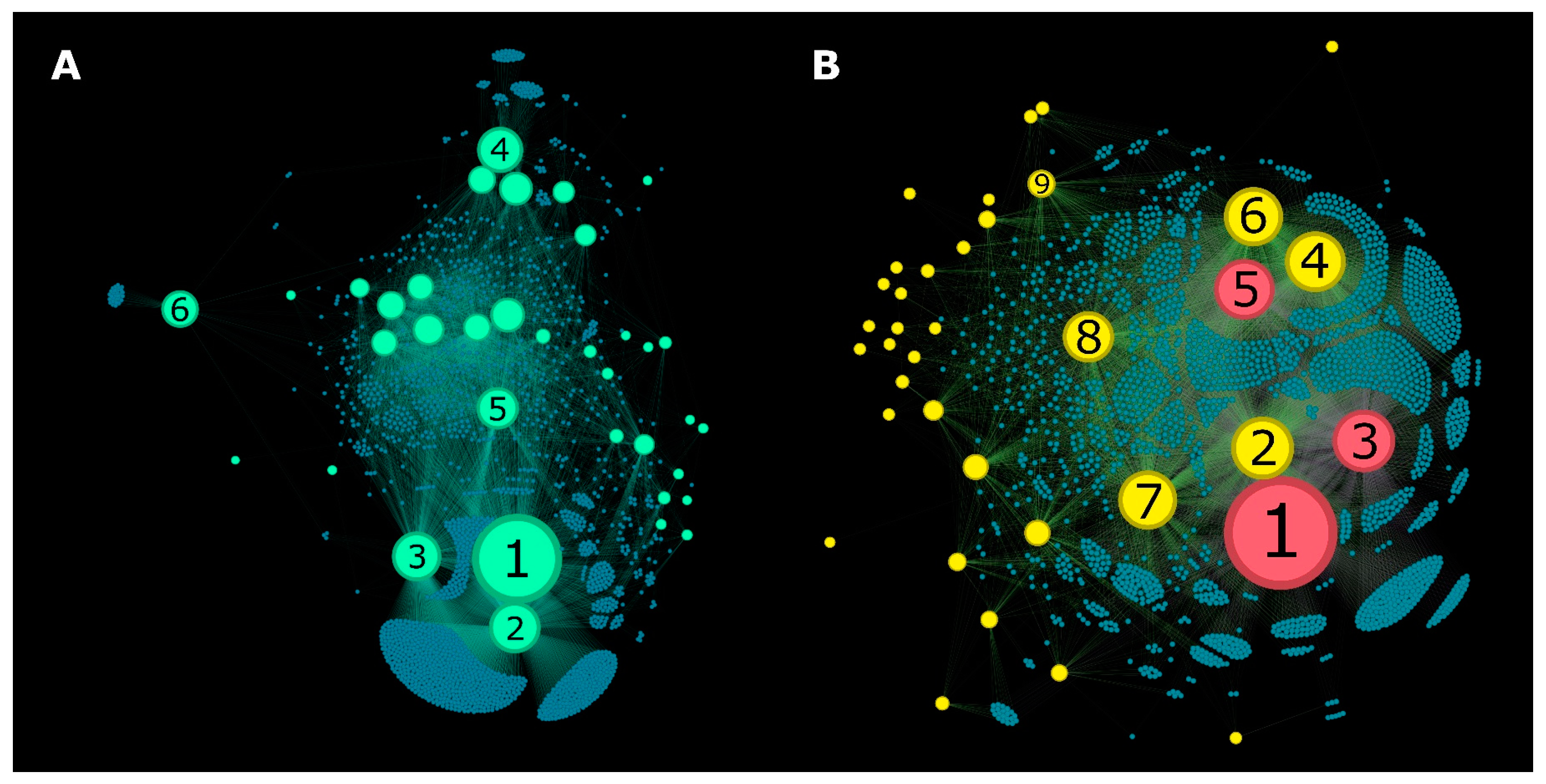
Figure 3. Metadata networks (METNs) based on (A) Origin and (B) Target. (A) Origin METN describes the origin of the hemolytic peptides (e.g., synthetic, isolated from Halocynthia aurantium, etc.). The dashed box represents the whole Origin METN whereas the bigger figure represents the central part of the Origin METN that was zoomed in for a better visualization. Blue-green nodes represent peptides while violet nodes represent the origin of the peptides. (B) Target METN describes the target of the hemolytic peptides (e.g., RBCs, Gram positive bacteria, etc.) which is a useful information when exploring associations between therapeutic and hemolytic activities. The dashed box represents the whole Target METN whereas the bigger figure represents the central part of the Target METN that was zoomed in for a better visualization. Blue-green nodes represent peptides whereas green nodes represent the reported target of the peptides. These networks were visualized in Gephi [40] using Force Atlas 2 layout [37] and edited with Inkscape [32].

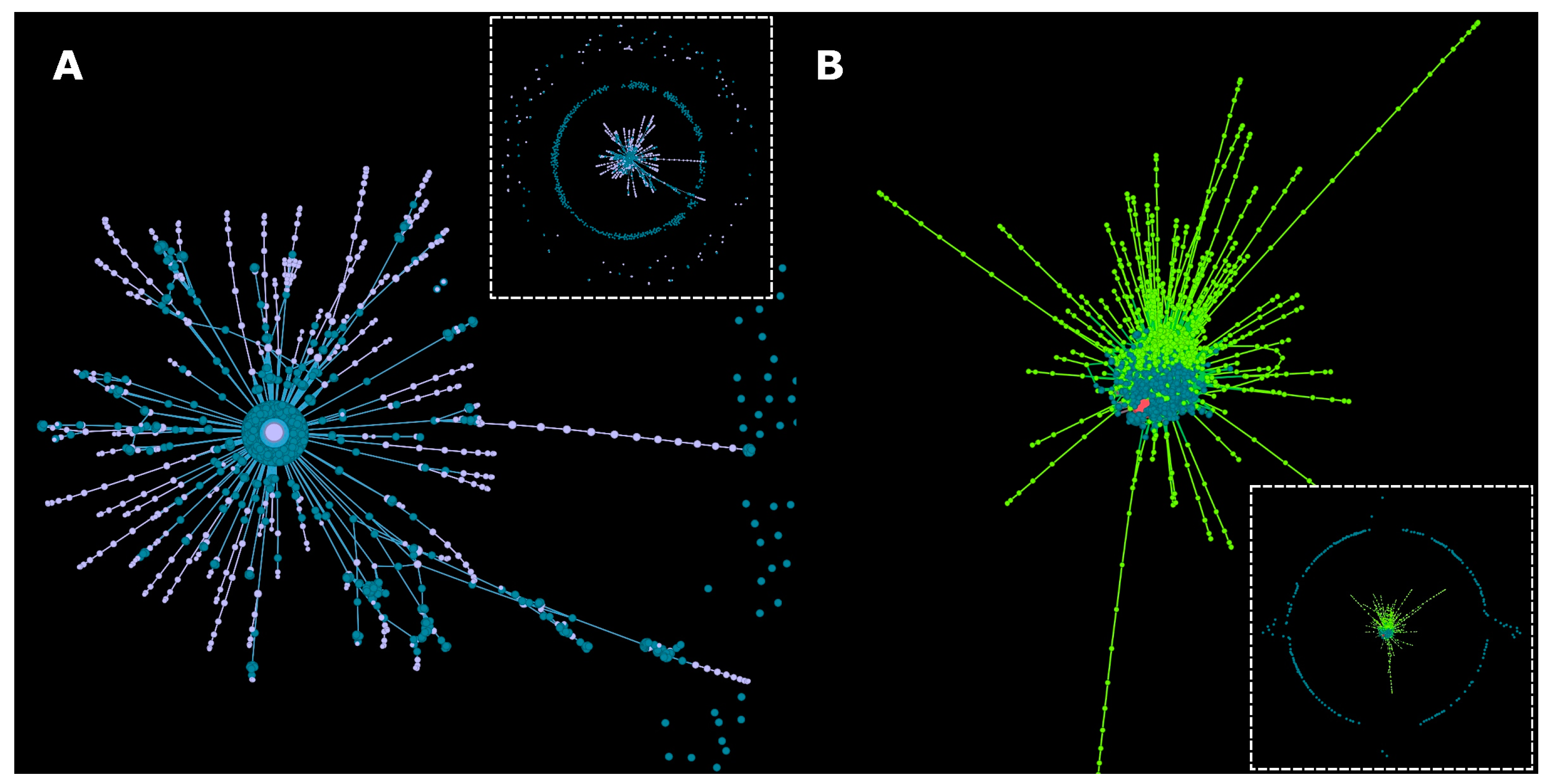
Figure 4. Global network parameters of HSPNs created with different metrics and similarity cutoff values t. ACC = Average Clustering Coefficient. This figure was created with ggplot2 R package [59] and edited with Inkscape [32].

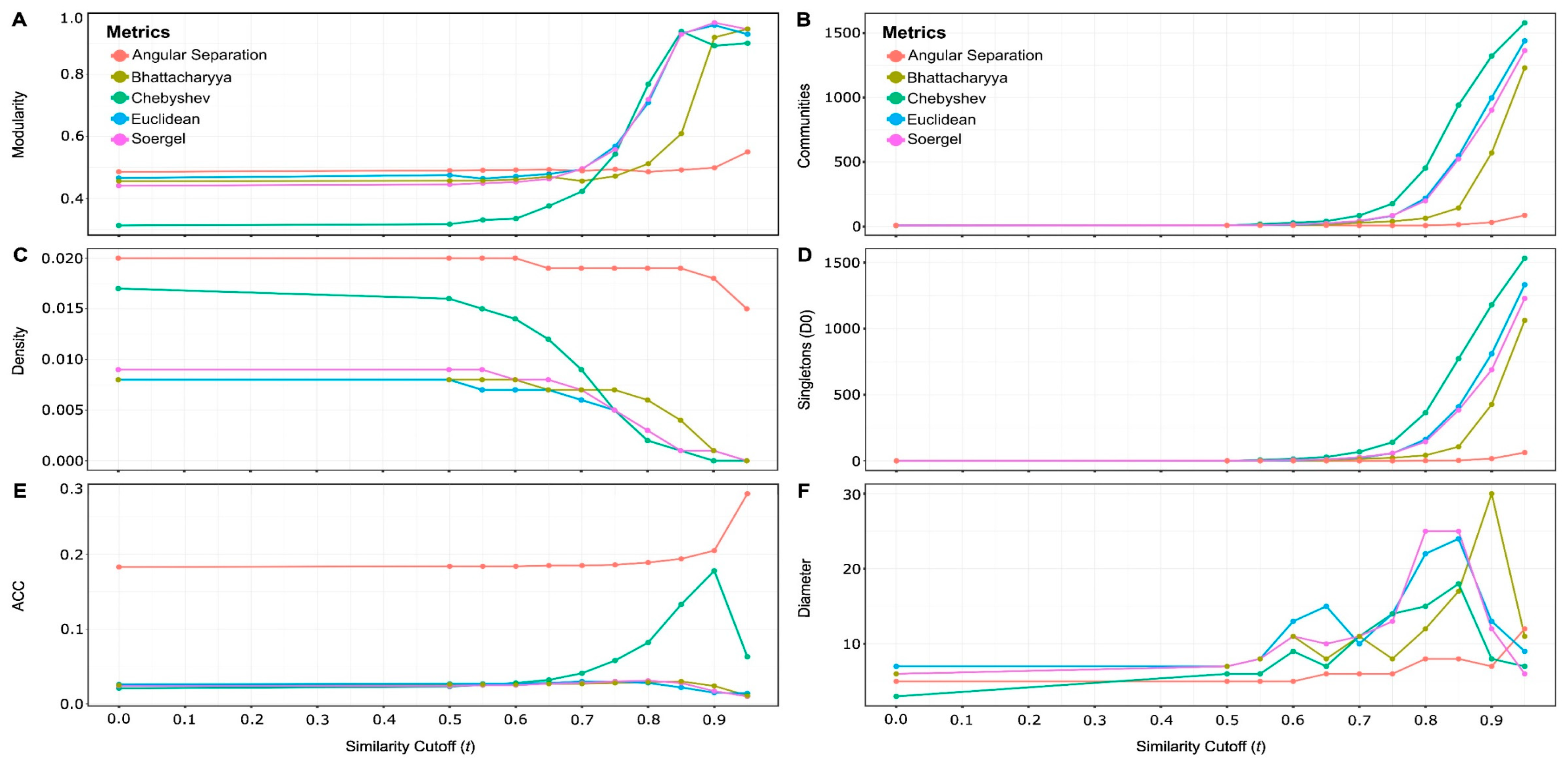
Figure 5. Probability of k (degree distribution) of the HSPNs with cutoff t = 0.00 (left) and with the best cutoff t (right) presented in Table 2. The average degree is presented next to the name of the corresponding network. (A) 0.00_AS: 32.15. (B) 0.90_AS: 30.44. (C) 0.00_Bh: 12.82. (D) 0.75_Bh: 11.37. (E) 0.00_Ch: 27.24. (F) 0.65_Ch: 20.31. (G) 0.00_Eu: 12.75. (H) 0.70_Eu: 10.30. (I) 0.00_So: 14.67. (J) 0.70_So: 11.56. This figure was created with ggplot2 R package [59] and edited with Inkscape [32].

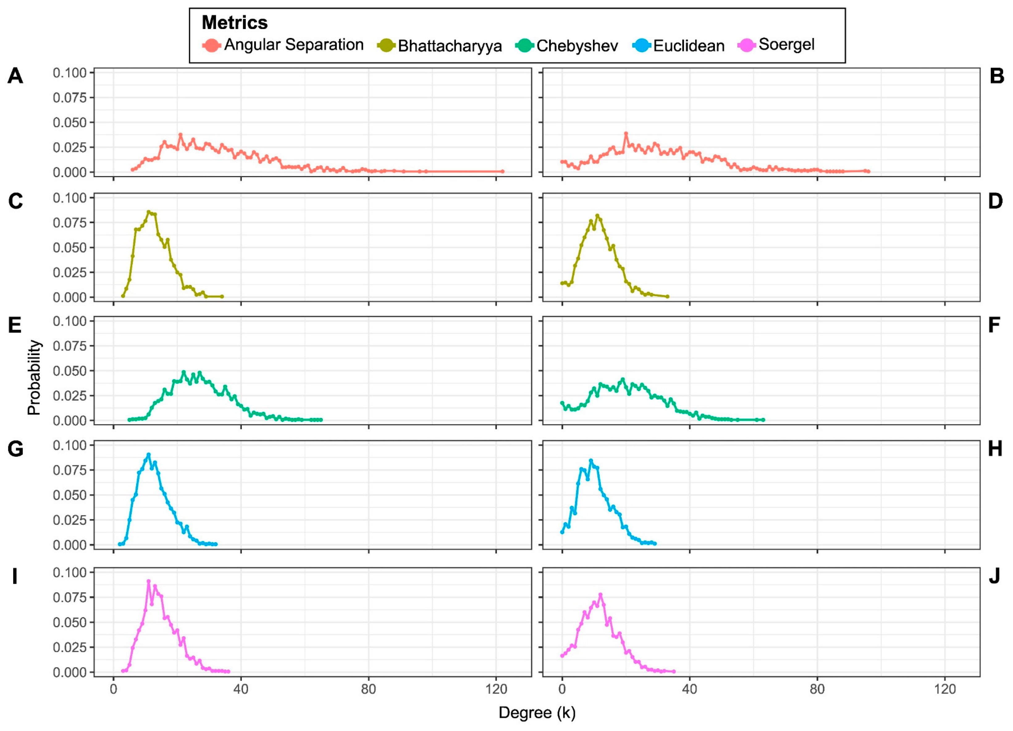
Figure 6. Graphical representation of HSPNs with t = 0.00 (left) and networks with the best t value for each metric (right). (A) 0.00_AS (B) 0.90_AS. (C) 0.00_Bh. (D) 0.75_Bh (E) 0.00_Ch. (F) 0.65_Ch (G) 0.00_Eu. (H) 0.70_Eu. (I) 0.00_So. (J) 0.70_So. Node colors represent communities of peptides and the size of the node represents the HB centrality value. Layout: Fruchterman-Reingold [39]. Networks were created with StarPep toolbox [25], visualized in Gephi [40] and edited with Inkscape [32].

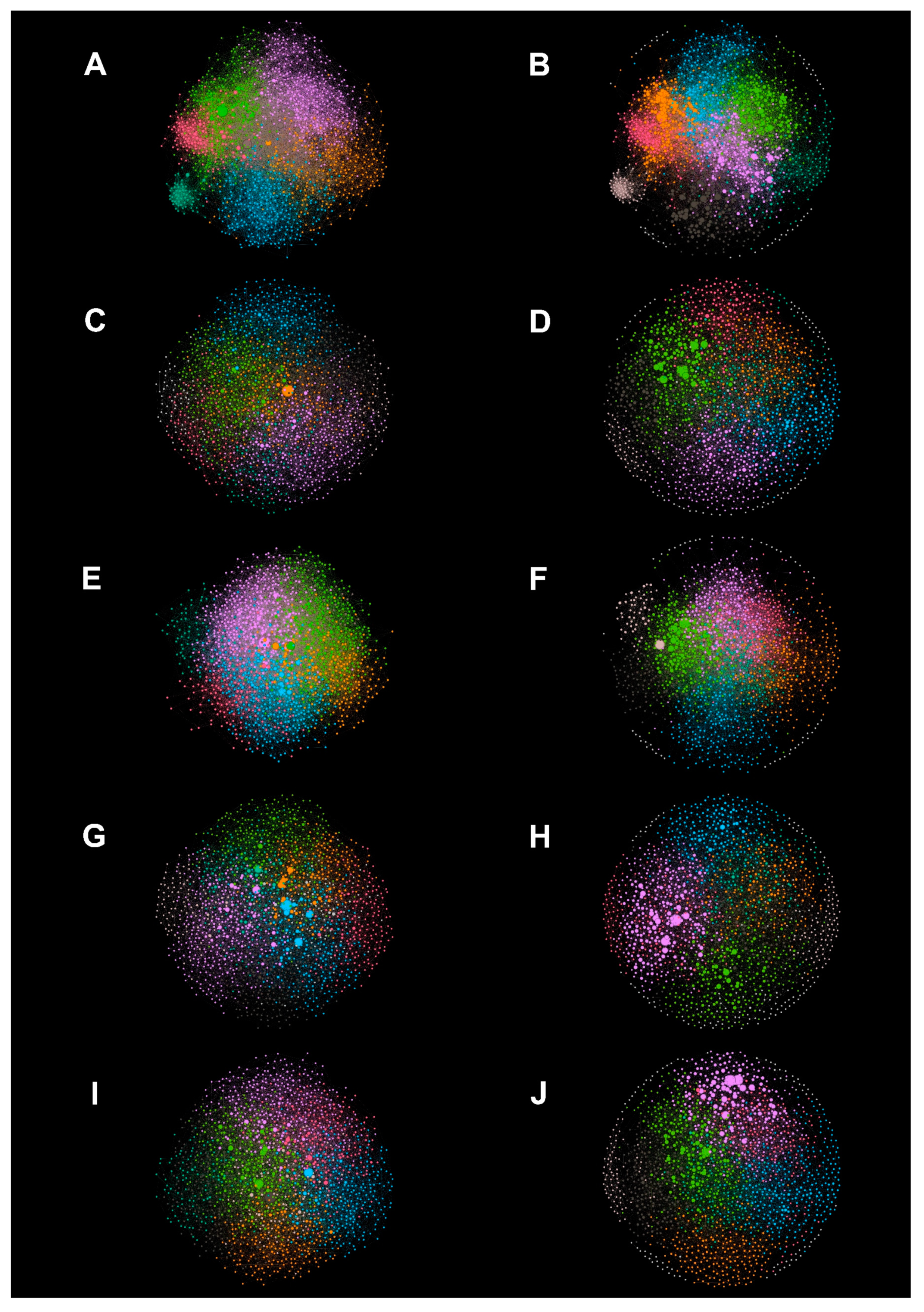
Figure 7. Pairwise Jaccard similarity coefficient (JSC) between scaffolds from networks constructed with different metrics when t = 0.00. (A,B) HB centrality. (C,D) HC centrality. (A,C) Global alignment. (B–D) Local alignment. The cutoff s represents the similarity cutoff applied to extract the scaffolds whereas the percentage in the y-axis represents the percentage of the JSC, which is the number of common peptides between a pair of scaffolds with respect to the union of the peptides of these scaffolds. The higher the percentage, the higher the number of common peptides between pairs of scaffolds. This figure was created with ggplot2 R package [59] and edited with Inkscape [32].

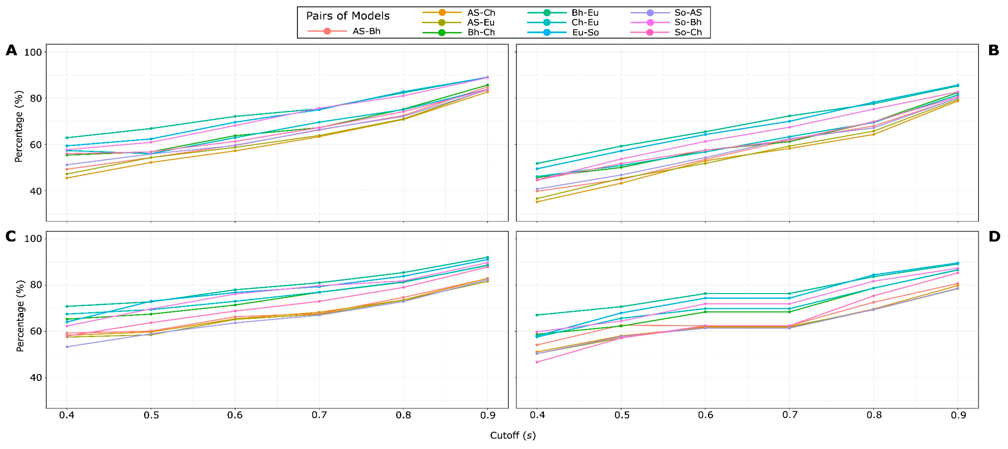
Figure 8. Pairwise Jaccard similarity coefficient (JSC) between scaffolds from networks constructed with the same metric but differing their t values (t = 0.00 vs. best t value). (A,B) HB centrality. (C,D) HC centrality. (A–C) Global alignment. (B–D) Local alignment. This figure was created with ggplot2 R package [59] and edited with Inkscape [32].

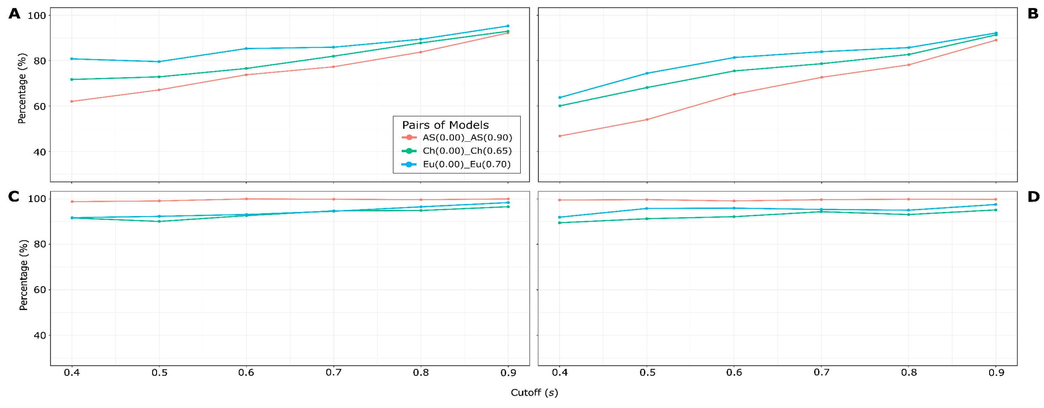
Figure 9. Pairwise Jaccard similarity coefficient (JSC) between scaffolds from networks constructed with the same metric but differing the alignment type. (A,B) HB centrality. (C,D) HC centrality. (A–C) networks with t = 0.00. (B–D) networks with best cutoff t: AS (0.90), Ch (0.65), Eu (0.70). This figure was created with ggplot2 R package [59] and edited with Inkscape [32].

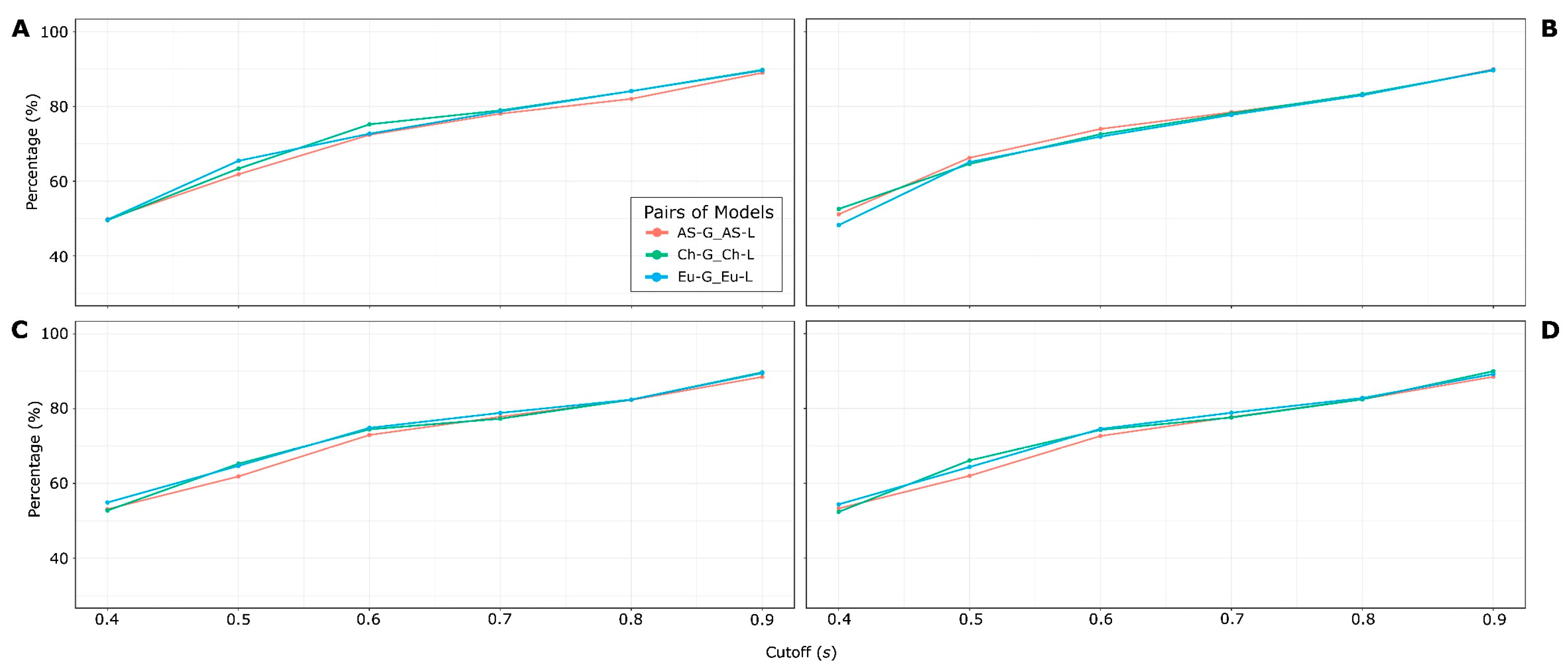
Figure 10. Size comparison of scaffold pairs generated from the network 0.00_AS. Pink area (G) represents the peptide sequences unique to the scaffold 0.00_AS_HB_G_0.40, green area (L) represents the sequences unique to the scaffold 0.00_AS_HB_L_0.40. The intersection of pink and green represents the number of common peptides between these two scaffolds. The area-proportional Venn diagram was created using DeepVenn [62] and edited with Inkscape [32].

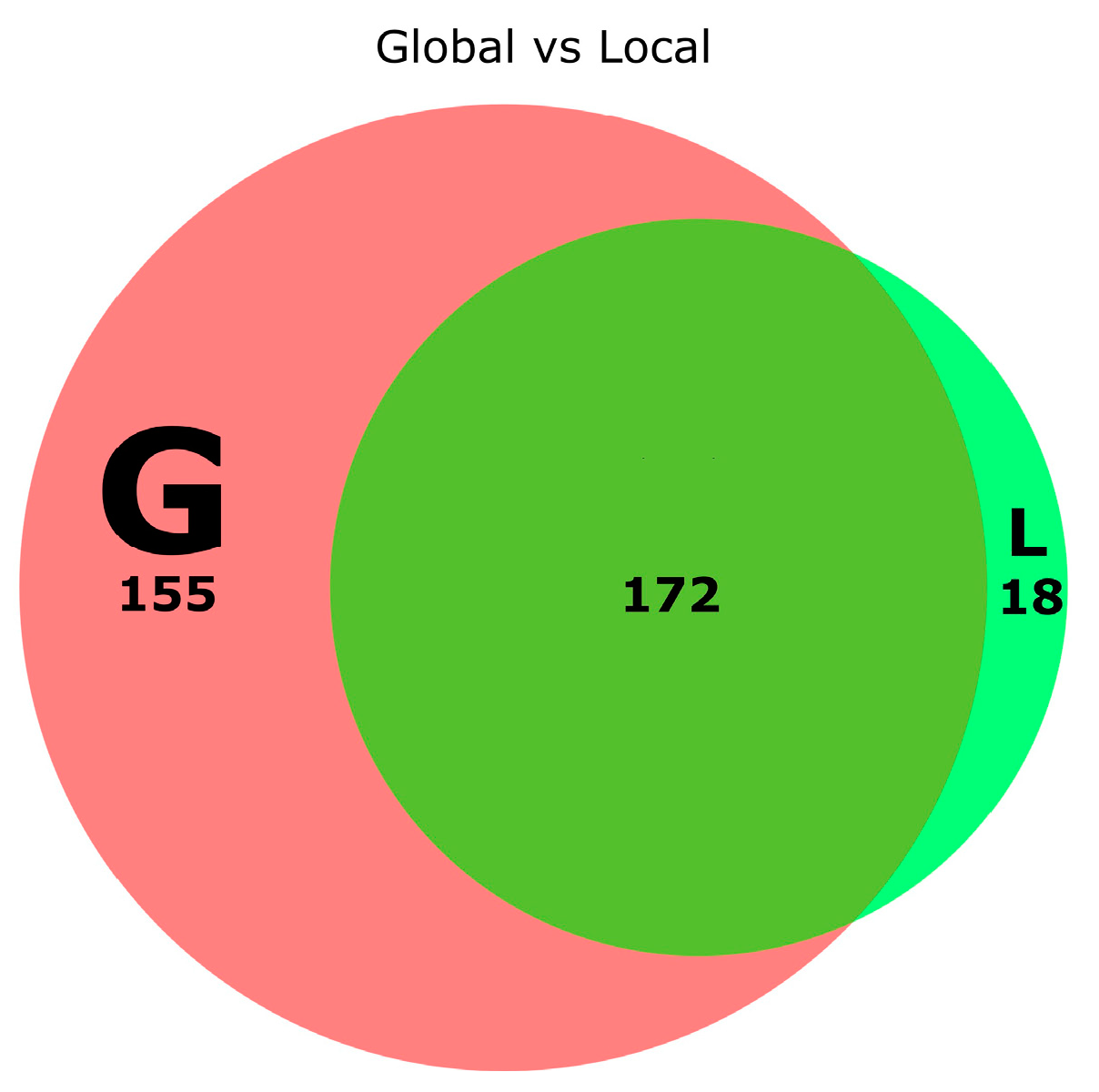
Figure 11. Pairwise Jaccard similarity coefficient (JSC) between scaffolds from networks constructed with the same metric but differing the centrality type. (A,B) Global alignment. (C,D) Local alignment. (A–C) networks with t = 0.00. (B–D) networks with best cutoff t: AS (0.90), Ch (0.65), Eu (0.70). This figure was created with ggplot2 R package [59] and edited with Inkscape [32].

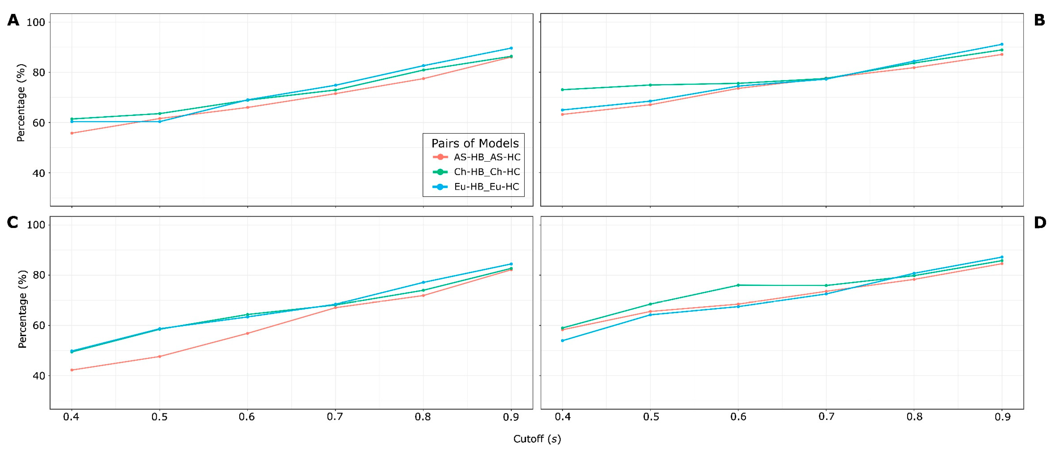
Figure 12. Barplot showing the coverage of the scaffolds 0.00_AS_HB_L at different s values. Scaffold representations are shown below their cutoff s values. This figure was created with ggplot2 R package [59] and edited with Inkscape [32].

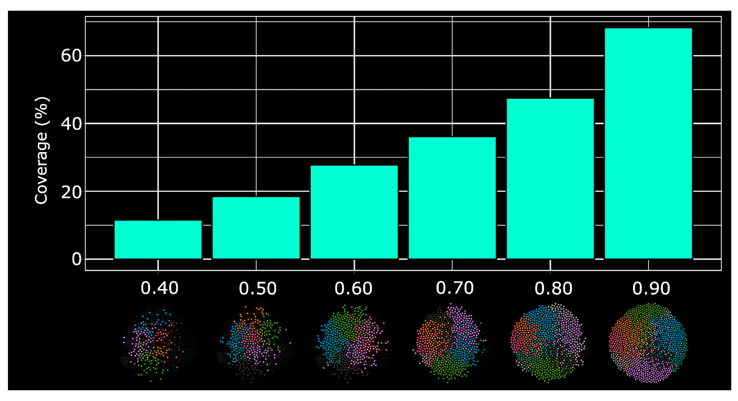
Table 1. (Dis)Similarity Measures used to Construct HSPNs.

Measure	Formula^a	Range^b	Average	Range
Angular Separation/[1-Cosine (Ochiai)] (AS)	$d_{X Y} = 1 - {C o s}_{X Y}$ where, ${C o s}_{X Y} = \frac{X Y}{‖X‖ ‖Y‖} = \frac{\sum_{j = 1}^{h} x_{j} y_{j}}{\sqrt{\sum_{j = 1}^{h} x_{j}^{2} \sum_{j = 1}^{h} y_{j}^{2}}}$	$[0,2]$
Bhattacharyya (Bh)	$d_{X Y} = \sqrt{\sum_{j = 1}^{h} {(\sqrt{x_{j}} - \sqrt{y_{j}})}^{2}}$	$[0, \infty)$	$\bar{d} = \frac{d_{X Y}}{\sqrt{n}}$	$[0, \infty)$
Chebyshev/Lagrange (Ch)	$d_{X Y} = m a x \{\|x_{j} - y_{j}\|\}$	$[0, \infty)$	$\bar{d} = \frac{d_{X Y}}{n^{\frac{1}{p}}}$	$[0, \infty)$
Euclidean (Eu)	$d_{X Y} = {(\sum_{j = 1}^{h} {\|x_{j} - y_{j}\|}^{2})}^{\frac{1}{2}}$	$[0, \infty)$	$\bar{d} = \frac{d_{X Y}}{n^{\frac{1}{p}}}$	$[0, \infty)$
Soergel (So)	$d_{X Y} = \frac{1}{n} \sum_{j = 1}^{h} \frac{\|x_{j} - y_{j}\|}{m a x \{x_{j}, y_{j}\}}$	$[0,1]$	$\bar{d} = \frac{d_{X Y}}{n}$	$[0, \frac{1}{n}]$

^a The variables x_j and y_j are the values of the molecular descriptor j of the peptides m and n, respectively. Peptides m and n are represented by the feature vectors X and Y. The h value is the number of peptide’s features. The p value in the Euclidean metric is 2, whereas for Chebyshev

p \to \infty

. ^b“Range” refers to “range” and not to “rank” and is defined as Range = max{x_j} – min {x_j}.

Table 2. Global network parameters of HSPNs with their best t values and their corresponding network at t = 0.00.

No	Metrics	Cutoff (t)	Edges	Modularity	Density	ACC	Clusters (no D0)	Singletons (D0)	Diameter
1	Angular Separation	0.00	26471	0.490	0.020	0.183	8	0	5
2	Angular Separation	0.90	25065	0.499	0.018	0.205	15	17	7
3	Bhattacharyya	0.00	10555	0.456	0.008	0.025	8	0	6
4	Bhattacharyya	0.75	9364	0.472	0.007	0.028	17	23	8
5	Chebyshev	0.00	22431	0.313	0.017	0.021	7	0	3
6	Chebyshev	0.65	16809	0.376	0.012	0.032	12	29	7
7	Euclidean	0.00	10498	0.466	0.008	0.026	9	0	7
8	Euclidean	0.70	8482	0.494	0.006	0.030	20	21	10
9	Soergel	0.00	12077	0.441	0.009	0.024	8	0	6
10	Soergel	0.70	9521	0.496	0.007	0.028	17	27	11

Table 3. Motifs discovered by STREME using the community information from the HSPNs created using Angular Separation, Chebyshev and Euclidean metrics with t = 0.00.

No	Metric	Motif	Cluster	Cluster size	Matches in positive seqs.	Matches in control seqs.	Sites^a (%)	p-value	E-value
1	Angular Separation (AS)	WKSFLK	0	223	81	3	36.3	0.023	0.120
2		SLCEZ	1	140	61	0	43.6	0.005	0.048
3		GLPV	3	61	45	0	73.8	0.017	0.140
4		CGETCV	3	61	56	0	91.8	0.017	0.140
5		WKKI	5	255	88	10	34.5	0.025	0.120
6	Chebyshev (Ch)	GILDTJ	1	304	72	0	23.7	0.010	0.073
7		MFTLK	2	246	57	0	23.2	0.034	0.310
8		CSW	4	59	44	0	74.6	0.024	0.190
9		VCGETC	4	59	49	0	83.1	0.004	0.032
10		LCYCRR	6	150	41	0	27.3	0.031	0.150
11	Euclidean (Eu)	LKGAGK	0	339	74	0	21.8	0.004	0.047
12		VCTRN	1	101	76	0	75.2	0.004	0.038
13		WKSFJK	5	220	45	0	20.5	0.015	0.092
14		LHTAKK	5	220	54	0	24.5	0.002	0.011
15		CYCRR	7	189	43	0	22.8	0.032	0.160

^aSites represents the percentage of positive peptides matching the motif.

Table 4. Hemolytic motifs that have all their E-value ranks less than 37 sorted by their average enrichment ratio of the three datasets: HemoPI-1, StarPepDB and Big-Hemo. For the complete information about all motifs see SM5.2. Motifs highlighted in red are newly reported hemolytic motifs.

		HemoPI-1			StarPepDB			Big-Hemo
No.	Motif	ER^a	E-value	Rank^b	ER^a	E-value	Rank^b	ER^a	E-value	Rank^b
1	ALKAIS	3.66	1.92E-09	36	40.10	3.53E-21	35	3.32	8.48E-12	9
2	WKSFJK	19.20	2.80E-40	2	5.06	3.55E-158	1	4.94	6.01E-22	3
3	AKKAL	16.10	7.19E-29	11	3.33	6.66E-101	4	1.55	6.30E-04	24
4	LKKL	12.60	1.44E-31	4	3.62	2.65E-130	2	1.68	1.37E-08	12
5	ISWIK	7.86	5.69E-19	19	6.19	3.45E-59	15	2.51	4.45E-05	22
6	LHTA[KL]	3.94	1.90E-13	25	8.25	4.73E-27	29	3.74	1.76E-11	10
7	FLHSAK	7.04	1.82E-11	29	5.69	2.10E-45	21	1.95	1.14E-03	26
8	LWKT	7.25	4.60E-31	6	2.35	5.59E-55	18	3.50	2.59E-10	11
9	FLGTI	6.94	1.41E-14	22	2.15	1.18E-21	33	3.88	5.70E-24	2
10	KKILG	6.71	1.61E-26	13	3.29	3.56E-77	11	1.85	1.36E-07	13
11	KITK	6.99	5.48E-26	15	2.48	1.22E-57	16	2.05	1.68E-01	36
12	LGKL	5.47	1.14E-29	7	2.17	5.13E-87	8	3.34	5.48E-12	8
13	KWK	4.84	2.02E-31	5	3.97	1.22E-55	17	1.98	1.79E-07	15
14	KGAGK	5.13	2.35E-27	12	2.66	2.25E-43	22	2.81	2.43E-14	4
15	SWP	4.56	5.42E-26	14	3.76	7.67E-35	26	1.98	5.44E-03	28
16	LLKK	4.31	1.88E-34	3	3.82	1.35E-126	3	1.60	1.18E-01	35
17	[VI]LDTJ	3.02	4.39E-10	33	2.15	1.05E-40	23	4.27	1.58E-24	1
18	JGKL	4.07	1.38E-29	8	2.32	8.01E-90	7	1.71	2.12E-07	17
19	VLK	3.00	8.34E-17	20	2.06	9.64E-64	14	1.88	1.52E-07	14
20	PKIF	2.89	1.05E-14	21	2.19	3.22E-46	20	1.47	4.79E-03	27

^aER = Enrichment Ratio. ^bSEA returns motifs ranked according to their associated E-value.

Table 5. An example of the use of hemolytic motifs as toxic signatures. The table shows pairs of hemolytic peptides with similar lengths showing different hemolytic activities based on the number of hemolytic motifs. Motifs in red are newly reported hemolytic motifs.

No.	Sequence	Length	No. Motifs	Consensus Motifs	Hemolytic Activity	Ref
1	RGLRRLGRKIAHGVKKYGPTVKRIKRKA	28	0		Not active at 100 µM	[63]
2	KWKSFLKTFKSAAKTVLHTALKAISS	28	4	WKSFJK, LHTA[KL], KWK, ALKAIS	50% hemolysis at 16 µM	[64]
3	MASRAARLAARLARLALRAL	20	0		1% hemolysis at 92.95 µM	[65]
4	ALWMTLLKKVLKAAAKAALN	20	4	LLKK, VLK, AAAK, ALW	50% hemolysis at 5 ± 1 µM	[66]
5	KRLFRRWQWRMKKY	14	0		Not active up to 100 µM	[67]
6	WCYCRRRFCVCVGR	14	3	RFC, CYCR, CRR	> 50% hemolytic at 44.3 µM	[68]

Disclaimer/Publisher’s Note: The statements, opinions and data contained in all publications are solely those of the individual author(s) and contributor(s) and not of MDPI and/or the editor(s). MDPI and/or the editor(s) disclaim responsibility for any injury to people or property resulting from any ideas, methods, instructions or products referred to in the content.

© 2024 by the authors. Licensee MDPI, Basel, Switzerland. This article is an open access article distributed under the terms and conditions of the Creative Commons Attribution (CC BY) license (https://creativecommons.org/licenses/by/4.0/).

Copyright: This open access article is published under a Creative Commons CC BY 4.0 license, which permit the free download, distribution, and reuse, provided that the author and preprint are cited in any reuse.

Downloads

210

Views

294

Comments

Subscription

Notify me about updates to this article or when a peer-reviewed version is published.

MDPI Initiatives

Important Links

Choose an area of interest and we will send you notifications of new preprints at your preferred frequency.

Disclaimer

Peptide Hemolytic Activity Analysis using Visual Data Mining of Similarity-based Complex Networks

Abstract

Keywords:

Subject:

1. Introduction

2. Materials and Methods

2.1 Datasets

2.2 Network Generation and Analysis

2.2.1. Metadata Networks (METNs)

2.2.2. Half-Space Proximal Networks (HSPNs)

2.2.3. Network Visualization

2.2.4. Selection of the best HSPNs

2.3 HSPNs Scaffold Extraction and Analysis

2.5. Motif Discovery and Enrichment

2.5.1. Motif Discovery

2.5.2. Motif Enrichment

3. Results and Discussion

3.1. Metadata Networks (METNs)

3.2. Half-Space Proximal Networks (HSPNs)

3.3. HSPNs Scaffolds

3.4. Hemolytic Motif Discovery and Enrichment

4. Conclusions

Supplementary Materials

Author Contributions

Funding

Institutional Review Board Statement

Informed Consent Statement

Data Availability Statement

Acknowledgments

Conflicts of Interest

References

MDPI Initiatives

Important Links

Subscribe