Flood Frequency Analysis Using the Gamma Family Probability Distributions

Cornel Ilinca; Cristian Gabriel Anghel

doi:10.20944/preprints202303.0320.v1

Submitted:

17 March 2023

Posted:

17 March 2023

You are already at the latest version

Abstract

This article presents six probability distributions from the Gamma family with three parameters, for the flood frequency analysis in hydrology. The choice of the Gamma family of statistical dis-tributions was driven by its frequent use in hydrology. In the Faculty of Hydrotechnics, the im-provement of the estimation of maximum flows and including the methodological bases for the realization of a regionalization study with the linear moments method with the corrected pa-rameters was researched, being an element of novelty. The linear moments method is better than MOM because it avoids the choice of skewness depending on the origin of the flows, practiced in Romania. The L-moments method conforms to the current trend for estimating the parameters of statistical distributions. Observed data from hydrometric stations are of relatively short length, so the statistical parameters that characterize them are of a sample that requires correction. The correction of the statistical parameters is proposed, using the method of least squares based on the inverse functions of the statistical distributions expressed with the frequency factor for L-moments. All the necessary elements for their use are presented like, quantile functions, the exact and ap-proximate relations for estimating parameters and frequency factors. A flood frequency analysis case study was carried out for the Ialomita river, to verify the proposed methodology. The per-formance of this distributions is evaluated using Kiling-Gupta and Nash-Sutcliff coefficients.

Keywords:

Kritsky-Menkel

;

Pearson

;

Wilson-Hilferty

;

Chi

;

Inverse Chi

;

Pseudo-Weibull

;

estimation parameters

;

corrected parameters

;

approximate form

;

method of ordinary moments

;

method of linear moments

;

the method of least squares

;

confidence interval

Subject:

Computer Science and Mathematics - Probability and Statistics

Introduction

The frequency analysis of extreme values in hydrology is of particular importance in the determination of the values with certain probability of occurrence, necessary in the management of water resources [1], human activities, design of hydrotechnical constructions [2,3], respectively the environment [4] and biodiversity protection, especially in the current context of climate change.

In most cases, the flood frequency analysis is performed using some of the well-known distributions in the statistical analysis of extreme values, such as Pearson III, Log-Pearson III, three parameters Log-Normal and GEV [5,6].

To estimate the parameters of these types of statistical distributions, the most used methods are the method of ordinary moments (MOM) and the method of linear moments (L-moments), the latter having the advantage that it is less influenced by the length of the data series [7,8,9,10] or the extreme values in the data series, in some cases outlier values requiring the elaboration of specific verification tests. However, a correction of the statistical parameters (

L_{1}, τ_{2}, τ_{3}

) of the short series of maximum flows is necessary, because they differ from those of the considered statistical population, that is, of the theoretical probability distribution function.

This article presents six useful distributions in hydrology, from the Gamma family, for the flood frequency analysis, such as: the Kristsky-Menkel distribution (KM), the Pearson III distribution (PE3) the Wilson-Hilferty distribution (WH), the CHI distribution (CHI), the Inverse CHI distribution (ICH), respectively Pseudo-Weibull distribution (PW). The inverse functions (quantiles) of the analyzed distributions do not have explicit forms, they are represented in this article with the help of the predefined function from Mathcad, which is equivalent to other functions from other dedicated programs (the Gamma.Inv function from Excel, etc.) or with the frequency factor, both for MOM and L-moments, which are presented in the Appendices B, C, D, E, F, depending on skewness (

C_{s}

) and L-skewness (

τ_{3}

), for the most common exceeding probabilities in hydrology.

The methods for estimating the parameters of these distributions are the method of ordinary moments (MOM) and the method of linear moments (L-moments). In general, to estimate the parameters, it is necessary to solve some nonlinear systems of equations, which leads to some difficulties in using these distributions. Thus, for the ease applications of these distributions, parameter approximation relations are presented, using polynomial, exponential or rational functions.

It should be mentioned that the proposed methodology differs from the classical one popularized by Hosking [7], by the fact that it brings a correction to the indicators obtained with the L-moments method, the method being more stable than other estimation methods but still requiring a certain correction for short data length.

New elements such as: the expressions of the cumulative complementary functions and the inverse functions for these distributions; the approximation relations for parameters estimation, for both MOM and L-moments; the distributions frequency factors for MOM and L-moments; the approximation relations for the frequency factors for most common probability in hydrology, for PE3, WH, CHI and PW, facilitates the ease of using these distributions in flood frequency analysis. Another new element is the correction of the statistical parameters of the data series for hydrometric stations with the method of least squares (LSM).

Thus, all these novelty elements for these distributions presented in Table 1 will help hydrology researchers to use these distributions easily.

The WH, CHI, ICH and PW distributions are used for the first time in the flood frequency analysis.

The KM distribution is used for the first time in the flood frequency analysis using L-moments method.

Analyzes were carried out for several characteristic hydrometric stations in Romania at all levels of altitude (mountainous, hilly and plain areas), implicitly for hydrographic basin areas from 100 km² to 10000 km². In order to verify the performances of the proposed distributions, a flood frequency analysis is carried out, using the Ialomita river, as a case study, because it is also presented in the Romanian normative NP 129/2011 [11].

The main objective of the article is the presentation of the methodological elements for the realization of a methodology based on the L-moment method necessary for the correction of some statistical indicators used later for regionalization, considering that in Romania there are no regulations regarding this analysis.

Comparing the results and choosing the best distribution is based on the performance indicators [12]: the Kling-Gupta coefficient (KGE), the Nash Sutcliffe coefficient (E), and

τ_{3} - τ_{4}

diagram.

The article is organized as follows. The description of methodology, the statistical distributions by presenting the density function, the complementary cumulative function and the quantile function, in Section 2.1. The presentation of the relations for exact calculation and the approximate relations for determining the parameters of the distributions, in Section 2.2. Presentation of a methodology for determining the maximum flows using the L-moments method and correcting the statistical parameters of the data string for hydro-metric stations with LSM, in Section 2.3. Case study by applying these distributions in flood frequency analysis for the Ialomita river, in Section 3. Results, discussions and conclusions, in Sections 4 and 5.

Methodology

In various scientific materials [7,8,9,13,14] MOM was presented compared to the L-moments method showing the advantages of the latter. However, a more mathematically rigorous presentation is needed to see the differences and advantages applied for three-parameter distributions.

In Table 2 presents the statistical parameters used for the use of three-parameter distributions [7].

where,

m_{1}, m_{2}, m_{3}

represent the first three centered ordinary moments;

L_{1}, L_{2}, L_{3}

represent the first three moments obtained based on the L-moments method [7,8,14];

μ, σ, ξ

represents the expected value, standard deviation, respectively the multiplication coefficient chosen according to the origin of the maximum flows [1,14,15,16].

Based on the inverse function of the distribution, these statistical parameters can be expressed as:

μ = L_{1} = \int_{0}^{1} x (p) d p

(1)

σ = \sqrt{\int_{0}^{1} {(x (p) - μ)}^{2}} d p

(2)

C_{s} = \frac{1}{σ^{3}} \cdot \int_{0}^{1} {(x (p) - μ)}^{3} d p

(3)

L_{2} = \int_{0}^{1} x (p) \cdot (1 - 2 \cdot p) d p

(4)

L_{3} = \int_{0}^{1} x (p) \cdot (1 - 6 \cdot p + 6 \cdot p^{2}) d p

(5)

In Romania, the calibration of parameters with MOM is performed using moments of first and second order, while the moment of third order is ignored by choosing skewness by multiplying the coefficient of variation [16].

A greater stability of the distribution is obtained knowing that the parameters of the distribution curves are different from those of the observed data, especially due to the small length, an aspect defined by the Empirical Law of Averages.

In fact, the moment of the third order requires a very large series of values (n≥100), thus the need to approximate it by knowing the statistical characteristics depending on the climate correlated with the physical-geographical conditions.

In the INHGA methodology for sections that are not monitored and have a relatively small hydrographic basin area, but that do not comply with [16], the coefficient of variation is ignored, adopting the value 1, without considering a proposed regionalization of it [17], leading to very large errors regarding the determination of maximum flows.

It is observed that the skewness is taken as a function of the coefficient of variation, trying to get a better estimate is often conservative, i.e., it results in higher values of the maximum flows compared to other more precise estimates, such as the least squares method (LSM). This aspect is for the benefit of safety, but it is often economically prohibitive, especially for low exceedance probabilities used in hydraulic constructions (p≥5‰). In general, LSM is avoided [1] to apply in the case of distributions from the Gamma family, because it results in very complex systems of nonlinear equations. This inconvenience is eliminated by using the nonlinear least squares method where the values are obtained by successive approximation (iterative methods).

Following the analysis of the inverse functions of the Gamma family distributions, analyzed in this article, it can be observed that they represent forms of the inverse function of cumulative probability distribution "parent", having the general expression presented in Figure 1.

Other particular forms of the inverse function are the distribution Pearson V (

c = γ

;

b = β

;

n = - 1

;

a = α - 1

) [18], Four Parameters Generalized Extreme Value (

c = γ

;

b = λ \cdot α^{- 1 / β}

;

n = β

;

a = α

) [19], Generalized Dual Gamma Extreme Values (

c = γ + \frac{β}{λ}

;

b = \frac{β}{λ}

;

n = - λ

;

a = α

) [20].

In the next section are presented the theoretical distributions from Gamma family analyzed in the research of the Faculty of Hydrotechnics regarding the regionalization studies of the maximum flows.

2.1. Probability Distributions

The probability density function,

f (x)

; the complementary cumulative distribution function,

F (x)

, and quantile function,

x (p)

, for analyzed distributions are:

Kritsky-Menkel (KM)

The distribution is, like the Pearson III distribution, a special case of the four-parameter exponential gamma distribution [19,21]. It also represents a reparametrized form of the generalized Gamma distribution [22]. It is also known as the generalized Weibull distribution, Stacy, hyper gamma, Nukiyama-Tanasawa, generalized semi-normal, modified gamma [19]. It was popularized in the analysis of maximum flows by Kristky and Menkel, becoming, starting with 1969, the standard distribution in the statistical analysis of maximum flows in the Soviet Union [22]. This was used in Romania as an alternative to Pearson III because it has positive lower bound. Its application was made using the linear interpolation of the values from the Kritsky-Menkel tables with values for

C_{v}

from 0 to 2, with a step of 0.1, and for skewness a coefficient of multiplication of the coefficient of variation, with values from 2 to 4 with a step of 0.5. Logarithmic interpolation of values is mandatory because linear interpolation causes errors.

f (x) = \frac{{(\frac{x}{x_{0}})}^{\frac{α}{λ} - 1} \cdot {(\frac{Γ (α + λ)}{Γ (α)})}^{\frac{α}{λ}}}{x_{0} \cdot |λ| \cdot Γ (α)} \cdot e^{- {(\frac{x}{x_{0}} \cdot \frac{Γ (α + λ)}{Γ (α)})}^{\frac{1}{λ}}}

(6)

f (x) = \frac{Γ (λ)}{x_{0} \cdot |λ| \cdot Γ (α) \cdot B e t a (λ, α)} \cdot {(\frac{x}{x_{0}} \cdot \frac{Γ (λ)}{B e t a (λ, α)})}^{\frac{α}{λ} - 1} \cdot e^{- {(\frac{x}{x_{0}} \cdot \frac{Γ (λ)}{B e t a (λ, α)})}^{\frac{1}{λ}}}

(7)

F (x) = \frac{Γ (α, {(\frac{x}{x_{0}} \cdot \frac{Γ (α + λ)}{Γ (α)})}^{\frac{1}{λ}})}{Γ (α)} = \frac{Γ (α, {(\frac{x}{x_{0}} \cdot \frac{Γ (λ)}{B e t a (α, λ)})}^{\frac{1}{λ}})}{Γ (α)}

(8)

x (p) = F^{- 1} (x) = x_{0} \cdot \frac{Γ (α)}{Γ (α + λ)} \cdot q g a m m a {(1 - p, α)}^{λ} = x_{0} \cdot \frac{B e t a (α, λ)}{Γ (λ)} \cdot q g a m m a {(1 - p, α)}^{λ}

(9)

x (p) = \exp (λ \cdot \ln (q g a m m a (1 - p, α)) + \ln (\frac{Γ (α - [α])}{Γ (λ + α - [α])}) + \sum_{i = 1}^{[α]} \ln (\frac{α - i}{λ + α - i}))

(10)

where

x_{0}

is the arithmetic mean,

α, λ

are the shape parameters;

[α]

is the whole part of the parameter;

x

can take any values in the range

0 < x < \infty

.;

λ

can be negative or positive. If

λ < 0

(negative skewness) then the first argument of the inverse of the distribution function Gamma,

Γ^{- 1} (1 - p; α)

becomes

Γ^{- 1} (p; α)

.

The built-in function from Mathcad

q g a m m a (1 - p, α) = γ^{- 1} ((1 - p) \cdot Γ (α), α)

returns the inverse cumulative probability distribution for probability p, for the Gamma distribution, where

γ^{- 1}

is the inverse of the lower incomplete gamma function, [23].

Pearson III (PE3)

The Pearson III represent a generalized form of the two-parameter Gamma distribution and a particular case of the four-parameter gamma distribution [14,24,25].

f (x) = \frac{{(x - γ)}^{α - 1}}{β^{α} \cdot Γ (α)} \cdot \exp (- \frac{x - γ}{β}) = \frac{1}{β} \cdot d g a m m a (\frac{x - γ}{β}, α)

(11)

F (x) = 1 - \int_{γ}^{x} f (x) d x = 1 - \frac{1}{β \cdot Γ (α)} \cdot {\int_{γ}^{x} (\frac{x - γ}{β})}^{α - 1} \cdot \exp (- \frac{x - γ}{β}) d x = \frac{Γ (α, \frac{x - γ}{β})}{Γ (α)}

(12)

x (p) = γ + β \cdot q g a m m a (1 - p, α)

(13)

where

α, β, γ

are the shape, the scale and the position parameters and

x

can take any values of range

γ < x < \infty

if

β > 0

or

- \infty < x < γ

if

β < 0

and

α > 0

;

μ, σ

represent the mean (expected value) and standard deviation. If

β < 0

(negative skewness) then the first argument of the inverse of the distribution function Gamma,

Γ^{- 1} (1 - p; α)

becomes

Γ^{- 1} (p; α)

.

In Romania, the Person III distribution is applied using the table of Foster-Ribkin. This table is improperly used with linear interpolation.

Wilson-Hilferty (WH)

The three-parameter Wilson-Hilferty distribution is a generalized form of the two-parameter Wilson-Hilferty distribution. Both are cases of Amoroso distribution [19].

f (x) = \frac{3 \cdot \exp (- {(\frac{x - γ}{β})}^{3})}{|β| \cdot Γ (α)} \cdot {(\frac{x - γ}{β})}^{3 \cdot α - 1}

(14)

F (x) = 1 - \int_{γ}^{x} \frac{3 \cdot \exp (- {(\frac{x - γ}{β})}^{3})}{|β| \cdot Γ (α)} \cdot {(\frac{x}{β})}^{3 \cdot α - 1} d x = \frac{Γ (α, {(\frac{x - γ}{β})}^{3})}{Γ (α)}

(15)

x (p) = γ + β \cdot \sqrt[3]{q g a m m a (1 - p, α)}

(16)

where

α, β, γ

are the shape, the scale and the position parameters;

α, β > 0

;

x

can take any values in the range

γ < x < \infty

.

CHI Distribution (CHI)

The Chi distribution is a particular case of the Amoroso distribution. It is also known as the Nakagami distribution [19].

f (x) = \frac{{(\frac{x - γ}{β})}^{α - 1}}{2^{\frac{α}{2} - 1} \cdot β \cdot Γ (\frac{α}{2})} \cdot \exp (- \frac{{(x - γ)}^{2}}{2 \cdot β^{2}})

(17)

F (x) = 1 - \int_{γ}^{x} \frac{{(\frac{x - γ}{β})}^{α - 1}}{2^{\frac{α}{2} - 1} \cdot β \cdot Γ (\frac{α}{2})} \cdot \exp (- \frac{{(x - γ)}^{2}}{2 \cdot β^{2}}) d x = \frac{Γ (\frac{α}{2}, \frac{{(x - γ)}^{2}}{2 \cdot β^{2}})}{Γ (\frac{α}{2})}

(18)

x (p) = γ + β \cdot \sqrt{2 \cdot g a m m a (1 - p, \frac{α}{2})}

(19)

where

α, β, γ

are the shape, the scale and the position parameters;

α, β > 0

;

x

can take any values in the range

γ < x < \infty

.

Inverse CHI Distribution (ICH)

The ICH distribution represents the inverse form of the CHI distribution. It is also known as the Inverse Nakagami distribution [19].

f (x) = \frac{2 \cdot \exp (- {(\frac{β}{x - γ})}^{2})}{|β| \cdot Γ (α)} \cdot {(\frac{β}{x - γ})}^{2 \cdot α + 1}

(20)

F (x) = 1 - \int_{γ}^{x} \frac{2 \cdot \exp (- {(\frac{β}{x - γ})}^{2})}{|β| \cdot Γ (α)} \cdot {(\frac{β}{x - γ})}^{2 \cdot α + 1} d x = \frac{Γ (α, {(\frac{β}{x - γ})}^{2})}{Γ (α)}

(21)

x (p) = γ + \frac{β}{\sqrt{q g a m m a (p, α)}}

(22)

where

α, β, γ

are the shape, the scale and the position parameters;

α, β > 0

;

x

can take any values in the range

γ < x < \infty

.

Pseudo-Weibull Distribution (PW)

The generalized Pseudo Weibull distribution is a particular case of the Amoroso distribution. It was presented for the first time by Viorel Gh. Voda in 1989 [26].

f (x) = \frac{1}{Γ (1 + \frac{1}{α})} \cdot |\frac{α}{β}| \cdot {(\frac{x - γ}{β})}^{α} \cdot \exp (- {(\frac{x - γ}{β})}^{α})

(23)

F (x) = 1 - \int_{γ}^{x} \frac{1}{Γ (1 + \frac{1}{α})} \cdot |\frac{α}{β}| \cdot {(\frac{x - γ}{β})}^{α} \cdot \exp (- {(\frac{x - γ}{β})}^{α}) d x = \frac{Γ (\frac{1}{α} + 1, {(\frac{x - γ}{β})}^{α})}{Γ (\frac{1}{α} + 1)}

(24)

x (p) = γ + β \cdot p g a m m a {(1 - p, (\frac{1}{α} + 1))}^{α}

(25)

where

α, β, γ

are the shape, the scale and the position parameters;

β > 0

;

x

can take any values in the range

γ < x < \infty

.

The quantile functions (inverse functions) of the distributions can also be expressed based on the frequency factor, both for MOM and L-moments, expressed with the inverse gamma function.

For the ease of application of the PE3, WH, CHI, PW distributions, the frequency factor can be approximately expressed with polynomial/rational functions, whose coefficients can be found in Appendix C, D, E, F, for the most common exceedance probability in hydrology.

Parameter estimation

The parameter estimation of the analyzed statistical distributions is presents for MOM and L-moments, two of the most used methods in hydrology for parameter estimation [13,24,27,28,29].

Kritsky-Menkel

The equations needed to estimate the parameters with MOM have the following expressions [22]:

μ = x_{0}

(26)

σ^{2} = x_{0}^{2} \cdot (\frac{Γ (α) \cdot Γ (α + 2 \cdot λ)}{Γ {(α + λ)}^{2}} - 1)

(27)

C_{s} = \frac{\frac{Γ (α + 3 \cdot λ)}{Γ (α)} + 2 \cdot \frac{Γ {(α + λ)}^{3}}{Γ {(α)}^{3}} - 3 \cdot \frac{Γ (α + 2 \cdot λ)}{Γ (α)} \cdot \frac{Γ (α + λ)}{Γ (α)}}{{(\frac{Γ (α + 2 \cdot λ)}{Γ (α)} - \frac{Γ {(α + λ)}^{2}}{Γ {(α)}^{2}})}^{1.5}}

(28)

For gamma function argument values greater than 171.6, the parameters are determined from the following system of nonlinear equations:

\frac{Γ (α - [α])}{Γ (α - [α] + λ)} \cdot \prod_{i = 1}^{[α]} \frac{α - i}{α + λ - i} \cdot \frac{Γ (α - [α] + 2 \cdot λ)}{Γ (α - [α] + λ)} \cdot \prod_{i = 1}^{[α]} \frac{α + 2 \cdot λ - i}{α + λ - i} - 1 = C_{v}^{2}

(29)

\frac{\begin{array}{l} {(\frac{Γ (α - [α])}{Γ (α - [α] + λ)} \cdot \prod_{i = 1}^{[α]} \frac{α - i}{α + λ - i})}^{2} \cdot \frac{Γ (α - [α] + 3 \cdot λ)}{Γ (α - [α] + λ)} \cdot \prod_{i = 1}^{[α]} \frac{α + 3 \cdot λ - i}{α + λ - i} - \\ 3 \cdot \frac{Γ (α - [α])}{Γ (α - [α] + λ)} \cdot \prod_{i = 1}^{[α]} \frac{α - i}{α + λ - i} \cdot \frac{Γ (α - [α] + 2 \cdot λ)}{Γ (α - [α] + λ)} \cdot \prod_{i = 1}^{[α]} \frac{α + 2 \cdot λ - i}{α + λ - i} + 2 \end{array}}{{(\frac{Γ (α - [α])}{Γ (α - [α] + λ)} \cdot \prod_{i = 1}^{[α]} \frac{α - i}{α + λ - i} \cdot \frac{Γ (α - [α] + 2 \cdot λ)}{Γ (α - [α] + λ)} \cdot \prod_{i = 1}^{[α]} \frac{α + 2 \cdot λ - i}{α + λ - i} - 1)}^{1.5}} = C_{s}

(30)

The parameter estimation with the L-moment method is done numerically (definite integrals) based on the equations using the quantile of the function.

\frac{Γ (α)}{Γ (λ + α)} \cdot \int_{0}^{1} q g a m m a {(1 - p, α)}^{λ} \cdot (1 - 2 \cdot p) \cdot d p = τ_{2}

(31)

\frac{Γ (α)}{Γ (λ + α)} \cdot \int_{0}^{1} q g a m m a {(1 - p, α)}^{λ} \cdot (6 \cdot p^{2} - 6 \cdot p + 1) \cdot d p = τ_{3} \cdot τ_{2}

(32)

where

τ_{2}, τ_{3}

represents the L-coefficient of variation, respectively the L-coefficient of skewness. The integrals are calculated numerically with the Gaussian Quadrature method.

Pearson III

For estimation with MOM, the distribution parameters have the following expressions [14,24,27,28]:

α = {(\frac{2}{C_{s}})}^{2}

(34)

β = \frac{σ}{2} \cdot C_{s}

(35)

γ = μ - α \cdot β

(36)

where

C_{s}

represents the skewness coefficient.

The parameter estimation with the L-moment method is done numerically (definite integrals) based on the equations using the quantile of the function.

An approximate form of parameter estimation can be adopted. The parameter

α

can be estimated using an approximation made up of two polynomial functions and one rational, depending on the definition domain of the estimated parameter [24].

Thus, for the estimation with the L-moments, the shape parameter

α

can be evaluated numerically with the following approximate forms, depending on L-skewness (

τ_{3}

):

if

0 < |τ_{3}| \leq \frac{1}{3}

:

α = \exp (\begin{array}{l} - 3.164791927 - 5.108735285 \cdot \ln (|τ_{3}|) - 4.116014079 \cdot \ln {(|τ_{3}|)}^{2} - \\ 2.985250105 \cdot \ln {(|τ_{3}|)}^{3} - 1.327399577 \cdot \ln {(|τ_{3}|)}^{4} - 0.373944875 \cdot \ln {(|τ_{3}|)}^{5} - \\ 0.065421611 \cdot \ln {(|τ_{3}|)}^{6} - 0.006508037 \cdot \ln {(|τ_{3}|)}^{7} - 0.000281969 \cdot \ln {(|τ_{3}|)}^{8} \end{array})

(37)

if

\frac{1}{3} < |τ_{3}| \leq \frac{2}{3}

:

α = \exp (\begin{array}{l} - 3.9918551 - 10.781466 \cdot \ln (|τ_{3}|) - 21.557807 \cdot \ln {(|τ_{3}|)}^{2} - \\ 33.8752604 \cdot \ln {(|τ_{3}|)}^{3} - 35.0641585 \cdot \ln {(|τ_{3}|)}^{4} - 22.921163 \cdot \ln {(|τ_{3}|)}^{5} - \\ 8.5491823 \cdot \ln {(|τ_{3}|)}^{6} - 1.3855653 \cdot \ln {(|τ_{3}|)}^{7} \end{array})

(38)

if

\frac{2}{3} < |τ_{3}| < 1

:

α = \frac{\begin{array}{l} 5.17817436 - 26.209448756 \cdot |τ_{3}| + 62.12494027 \cdot τ_{3}^{2} - 84.39423264 \cdot {|τ_{3}|}^{3} + \\ 67.08589624 \cdot τ_{3}^{4} - 29.150288079 \cdot {|τ_{3}|}^{5} + 5.364968945 \cdot τ_{3}^{6} \end{array}}{1 + 0.0005134 \cdot |τ_{3}| + 0.00063644 \cdot τ_{3}^{2}}

(39)

The scale parameter

β

and the position parameter

γ

are determined with the following expressions [24]:

β = L_{2} \cdot \sqrt{π} \cdot \frac{Γ (α)}{Γ (α + \frac{1}{2})}

(40)

γ = L_{1} - α \cdot β

(41)

Wilson-Hilferty

The equations needed to estimate the parameters with MOM have the following expressions:

μ = γ + \frac{β}{Γ (α)} \cdot Γ (α + \frac{1}{3})

(42)

σ^{2} = \frac{β^{2}}{Γ (α)} \cdot [Γ (α + \frac{2}{3}) - \frac{1}{Γ (α)} \cdot Γ {(α + \frac{1}{3})}^{2}]

(43)

C_{s} = \frac{α - \frac{3}{Γ {(α)}^{2}} \cdot Γ (α + \frac{2}{3}) \cdot Γ (α + \frac{1}{3}) + \frac{2}{Γ {(α)}^{3}} \cdot Γ {(α + \frac{1}{3})}^{3}}{\sqrt{\frac{Γ (α + \frac{2}{3})}{Γ (α)} - \frac{Γ {(α + \frac{1}{3})}^{2}}{Γ {(α)}^{2}}} \cdot (Γ (α + \frac{2}{3}) - \frac{Γ {(α + \frac{1}{3})}^{2}}{Γ (α)})}

(44)

The shape parameter can be obtained approximately depending on the skewness coefficient, using the following exponential function:

α = \exp (\begin{array}{l} - 1 . 6047146 - 1 . 2117058 \cdot \ln (C_{s}) - 2 . 4627986 \cdot 10^{- 1} \cdot \ln {(C_{s})}^{2} - \\ 3 . 0754515 \cdot 10^{- 2} \cdot \ln {(C_{s})}^{3} + 1 . 3529125 \cdot 10^{- 2} \cdot \ln {(C_{s})}^{4} + \\ 5 . 4495596 \cdot 10^{- 3} \cdot \ln {(C_{s})}^{5} + 6 . 0310303 \cdot 10^{- 7} \cdot \ln {(C_{s})}^{6} - \\ 3 . 5860178 \cdot 10^{- 4} \cdot \ln {(C_{s})}^{7} - 7 . 3564689 \cdot 10^{- 5} \cdot \ln {(C_{s})}^{8} - 4 . 7318329 \cdot 10^{- 6} \cdot \ln {(C_{s})}^{9} \end{array})

(45)

β = \frac{σ}{\sqrt{\frac{Γ (α + \frac{2}{3})}{Γ (α)} - \frac{Γ {(α + \frac{1}{3})}^{2}}{Γ {(α)}^{2}}}}

(46)

γ = μ - \frac{β \cdot Γ (α + \frac{1}{3})}{Γ (α)}

(47)

The parameter estimation with the L-moment method is done numerically (definite integrals) based on the equations using the quantile of the function.

An approximate form can be adopted based on the parameter estimation depending on L-skewness (

τ_{3}

), as follows:

if

0 < τ_{3} \leq 1 / 3

:

α = \exp (\begin{array}{l} - 4 . 16202506 - 3 . 261604018 \cdot \ln (τ_{3}) - 1 . 783702334 \cdot \ln {(τ_{3})}^{2} - \\ 0 . 770946644 \cdot \ln {(τ_{3})}^{3} - 0 . 221698815 \cdot \ln {(τ_{3})}^{4} - 0 . 041191426 \cdot \ln {(τ_{3})}^{5} - \\ 0 . 004665295 \cdot \ln {(τ_{3})}^{6} - 0 . 000287712 \cdot \ln {(τ_{3})}^{7} - 0 . 000007207 \cdot \ln {(τ_{3})}^{8} \end{array})

(48)

if

1 / 3 < τ_{3} \leq 2 / 3

:

α = \exp (\begin{array}{l} - 5 . 264027693 - 9 . 134993593 \cdot \ln (τ_{3}) - \\ 15 . 845477811 \cdot \ln {(τ_{3})}^{2} - 19 . 874003352 \cdot \ln {(τ_{3})}^{3} - \\ 15 . 495267042 \cdot \ln {(τ_{3})}^{4} - 6 . 752325319 \cdot \ln {(τ_{3})}^{5} - 1 . 255615645 \cdot \ln {(τ_{3})}^{6} \end{array})

(49)

if

2 / 3 < τ_{3} < 1

:

α = \exp (\begin{array}{l} - 7 . 712526023 - 93 . 06660109 \cdot \ln (τ_{3}) - 1 . 519099681 \cdot 10^{3} \cdot \ln {(τ_{3})}^{2} - \\ 1 . 602587644 \cdot 10^{3} \cdot \ln {(τ_{3})}^{4} - 1 . 041173897 \cdot 10^{5} \cdot \ln {(τ_{3})}^{4} - \\ 4 . 152482998 \cdot 10^{5} \cdot \ln {(τ_{3})}^{5} - 9 . 887282 \cdot 10^{5} \cdot \ln {(τ_{3})}^{6} - \\ 1 . 287749298 \cdot 10^{6} \cdot \ln {(τ_{3})}^{7} - 7 . 050767642 \cdot 10^{5} \cdot \ln {(τ_{3})}^{8} \end{array})

(50)

β = \frac{L_{2}}{\frac{Γ (α + \frac{1}{3})}{Γ (α)} - 2 \cdot z}

(51)

γ = L_{1} - \frac{β \cdot Γ (α + \frac{1}{3})}{Γ (α)}

(52)

where

z = \int_{0}^{1} q g a m m a {(1 - p, α)}^{1 / 3} \cdot p \cdot d p

, which can be approximated with the following equation:

z = \exp (\begin{array}{l} - 1 . 037385169 + 0 . 592727202 \cdot \ln (α) - 0 . 107494558 \cdot \ln {(α)}^{2} + \\ 0 . 027616773 \cdot \ln {(α)}^{3} - 0 . 002977204 \cdot \ln {(α)}^{4} - \\ 0 . 000546413 \cdot \ln {(α)}^{5} + 0 . 00123125 \cdot \ln {(α)}^{6} + \\ 0 . 000420922 \cdot \ln {(α)}^{7} + 0 . 000052295 \cdot \ln {(α)}^{8} + 0 . 000002315 \cdot \ln {(α)}^{9} \end{array})

(53)

An attempt was made to use a single approximation function for the entire L-skewness domain, but the results were unsatisfactory. Thus, considering the variation of the shape coefficient depending on L-skewness, the domain of L-skewness was discretized into three subdomains, similar to the structure of Hosking’s approximation for the shape parameter for estimation with L-moments for the Pearson III distribution [8,13].

CHI Distribution

The three equations needed to estimate the parameters with MOM are the following

μ = γ + \frac{β \cdot \sqrt{2} \cdot Γ (\frac{α + 1}{2})}{Γ (α)}

(54)

σ^{2} = \frac{2 \cdot β^{2}}{Γ (\frac{α}{2})} \cdot (Γ (\frac{α + 2}{2}) - \frac{1}{Γ (\frac{α}{2})} \cdot Γ {(\frac{α + 1}{2})}^{2})

(55)

C_{s} = \frac{Γ {(\frac{α}{2})}^{\frac{1}{2}} \cdot (Γ (\frac{α + 3}{2}) - \frac{3 \cdot Γ (\frac{α}{2} + 1) \cdot Γ (\frac{α + 1}{2})}{Γ (\frac{α}{2})} + 2 \cdot \frac{Γ {(\frac{α + 1}{2})}^{3}}{Γ {(\frac{α}{2})}^{2}})}{{(Γ (\frac{α}{2} + 1) - \frac{Γ {(\frac{α + 1}{2})}^{2}}{Γ (\frac{α}{2})})}^{1.5}}

(56)

The shape parameter can be obtained approximately depending on the skewness coefficient, using the following exponential function:

α = \exp (\begin{array}{l} - 0 . 007238125 - 1 . 535608574 \cdot \ln (C_{s}) - 0 . 071523471 \cdot \ln {(C_{s})}^{2} - \\ 0 . 081440908 \cdot \ln {(C_{s})}^{3} + 0 . 022903868 \cdot \ln {(C_{s})}^{4} + \\ 0 . 011332187 \cdot \ln {(C_{s})}^{5} - 0 . 004439425 \cdot \ln {(C_{s})}^{6} - \\ 0 . 000839157 \cdot \ln {(C_{s})}^{7} + 0 . 000512936 \cdot \ln {(C_{s})}^{8} - \\ 0 . 000017606 \cdot \ln {(C_{s})}^{9} - 0 . 000028015 \cdot \ln {(C_{s})}^{10} \end{array})

(57)

β = \frac{σ}{\sqrt{\frac{2 \cdot Γ (\frac{α}{2} + 1)}{Γ (\frac{α}{2})} - \frac{2 \cdot Γ {(\frac{α + 1}{2})}^{2}}{Γ {(\frac{α}{2})}^{2}}}}

(58)

γ = μ - \frac{β \cdot \sqrt{2} \cdot Γ (\frac{α + 1}{2})}{(\frac{α}{2})}

(59)

The parameter estimation with the L-moment method is done numerically (definite integrals) based on the equations using the quantile of the function.

An approximate form can be adopted based on the parameter estimation depending on L-skewness (

τ_{3}

), as follows:

if

0 < τ_{3} \leq 1 / 3

:

α = \exp (\begin{array}{l} - 1 . 906990611 - 0 . 106292205 \cdot \ln (τ_{3}) + 2 . 073034826 \cdot \ln {(τ_{3})}^{2} + \\ 1 . 554031981 \cdot \ln {(τ_{3})}^{3} + 0 . 557748563 \cdot \ln {(τ_{3})}^{4} + \\ 0 . 093813202 \cdot \ln {(τ_{3})}^{5} + 0 . 006046746 \cdot \ln {(τ_{3})}^{6} \end{array})

(60)

if

1 / 3 < τ_{3} < 1

:

α = \exp (\begin{array}{l} - 5 . 833505729 - 44 . 920603717 \cdot \ln (τ_{3}) - \\ 344 . 189211489 \cdot \ln {(τ_{3})}^{2} - 1 . 714208624 \cdot 10^{3} \cdot \ln {(τ_{3})}^{3} - \\ 5 . 335469552 \cdot 10^{3} \cdot \ln {(τ_{3})}^{4} - 1 . 052048531 \cdot 10^{4} \cdot \ln {(τ_{3})}^{5} - \\ 1 . 311917766 \cdot 10^{4} \cdot \ln {(τ_{3})}^{6} - 1 . 001341648 \cdot 10^{4} \cdot \ln {(τ_{3})}^{7} - \\ 4 . 26546763 \cdot 10^{3} \cdot \ln {(τ_{3})}^{8} - 776 . 287194577 \cdot \ln {(τ_{3})}^{9} \end{array})

(61)

β = \frac{L_{2}}{\frac{\sqrt{2} \cdot Γ (\frac{α + 1}{2})}{Γ (\frac{α}{2})} - 2 \cdot \sqrt{2} \cdot z}

(62)

γ = L_{1} - \frac{β \cdot \sqrt{2} \cdot Γ (\frac{α + 1}{2})}{Γ (\frac{α}{2})}

(63)

where

z = \int_{0}^{1} \sqrt{q g a m m a (1 - p, \frac{α}{2})} \cdot p \cdot d p

, which can be approximated with the following equation:

z = \exp (\begin{array}{l} - 1 . 800405366 + 1 . 030861358 \cdot \ln (α) - 0 . 170031489 \cdot \ln {(α)}^{2} + 0 . 018376595 \cdot \ln {(α)}^{3} + \\ 0 . 005413992 \cdot \ln {(α)}^{4} - 0 . 001474816 \cdot \ln {(α)}^{5} - 0 . 00018822 \cdot \ln {(α)}^{6} + \\ 0 . 000076011 \cdot \ln {(α)}^{7} + 0 . 000002634 \cdot \ln {(α)}^{8} - 0 . 000001551 \cdot \ln {(α)}^{9} \end{array})

(64)

Inverse CHI Distribution

The three equations needed to estimate the parameters with MOM are the following

μ = γ + \frac{β}{Γ (α)} \cdot Γ (α - \frac{1}{2})

(65)

σ^{2} = \frac{β^{2}}{α - 1} - \frac{4 \cdot β^{2} \cdot Γ {(α + \frac{1}{2})}^{2}}{{(2 \cdot α - 1)}^{2} \cdot Γ {(α)}^{2}}

(66)

C_{s} = \frac{\frac{Γ (α - \frac{3}{2})}{Γ (α)} - \frac{3}{Γ {(α)}^{2}} \cdot Γ (α - 1) \cdot Γ (α - \frac{1}{2}) + \frac{2}{Γ {(α)}^{3}} \cdot Γ {(α - \frac{1}{2})}^{3}}{{(\frac{1}{α - 1} - \frac{4 \cdot Γ {(α + \frac{1}{2})}^{2}}{(2 \cdot α - 1) \cdot Γ {(α)}^{2}})}^{1.5}}

(67)

The shape parameter can be obtained approximately depending on the skewness coefficient, using the following exponential function:

α = \exp (\begin{array}{l} 2.1090657 - 1.5242827 \cdot \ln (C_{s}) + 3.4953121 \cdot 10^{- 1} \cdot \ln {(C_{s})}^{2} + \\ 1.0907394 \cdot 10^{- 1} \cdot \ln {(C_{s})}^{3} - 2.0678665 \cdot 10^{- 2} \cdot \ln {(C_{s})}^{4} - \\ 2.7787718 \cdot 10^{- 2} \cdot \ln {(C_{s})}^{5} - 6.6917784 \cdot 10^{- 4} \cdot \ln {(C_{s})}^{6} + \\ 5.9641479 \cdot 10^{- 3} \cdot \ln {(C_{s})}^{7} + 2.8113899 \cdot 10^{- 4} \cdot \ln {(C_{s})}^{8} - \\ 7.543052 \cdot 10^{- 4} \cdot \ln {(C_{s})}^{9} + 7.5164824 \cdot 10^{- 5} \cdot \ln {(C_{s})}^{10} \end{array})

(68)

β = \frac{σ}{\sqrt{(\frac{1}{α - 1} - \frac{4 \cdot Γ {(α + 0.5)}^{2}}{{(2 \cdot α - 1)}^{2} \cdot Γ {(α)}^{2}})}}

(69)

γ = μ - \frac{β}{Γ (α)} \cdot Γ (α - 0.5)

(70)

The parameters estimation with the L-moment method is done numerically (definite integrals) based on the equations using the quantile of the function.

An approximate form can be adopted based on the parameter estimation depending on L-skewness (

τ_{3}

), as follows:

α = \exp (\begin{array}{l} - 0 . 690555146 - 0 . 670486598 \cdot \ln (τ_{3}) + 1 . 3711601 \cdot \ln {(τ_{3})}^{2} + \\ 1 . 849011273 \cdot \ln {(τ_{3})}^{3} + 1 . 647100669 \cdot \ln {(τ_{3})}^{4} + \\ 0 . 821076191 \cdot \ln {(τ_{3})}^{5} + 0 . 22736483 \cdot \ln {(τ_{3})}^{6} + \\ 0 . 032883695 \cdot \ln {(τ_{3})}^{7} + 0 . 001941076 \cdot \ln {(τ_{3})}^{8} \end{array})

(71)

β = \frac{L_{2}}{\frac{Γ (α - \frac{1}{2})}{Γ (α)} - 2 \cdot z}

(72)

γ = L_{1} - \frac{β \cdot Γ (α - \frac{1}{2})}{Γ (α)}

(73)

where,

z = \frac{2 . 930815576 \cdot 10^{3} + 1 . 069477959 \cdot 10^{3} \cdot α - 28 . 265461564 \cdot α^{2} + 0 . 352559915 \cdot α^{3}}{1 + 7 . 389749366 \cdot 10^{3} \cdot α}

(74)

Pseudo-Weibull Distribution

The three equations needed to estimate the parameters with MOM are the following

μ = γ + \frac{β \cdot 2^{\frac{2}{α} + \frac{1}{2}} \cdot Γ (\frac{1}{α} + \frac{1}{2})}{\sqrt{2 \cdot π}}

(75)

σ^{2} = \frac{β^{2} \cdot 3^{\frac{3}{α} + \frac{1}{2}} \cdot Γ (\frac{1}{α} + \frac{1}{3}) \cdot Γ (\frac{1}{α} + \frac{2}{3})}{2 \cdot π} - \frac{β^{2} \cdot 2^{\frac{4}{α}} \cdot Γ {(\frac{1}{α} + \frac{1}{2})}^{2}}{π}

(76)

C_{s} = \frac{2 \cdot Γ {(\frac{1}{α})}^{2} \cdot Γ (\frac{4}{α}) + 8 \cdot Γ {(\frac{2}{α})}^{3} - 9 \cdot Γ (\frac{1}{α}) \cdot Γ (\frac{2}{α}) \cdot Γ (\frac{3}{α})}{4 \cdot {(\frac{3}{4} Γ (\frac{1}{α}) \cdot Γ (\frac{3}{α}) - Γ {(\frac{2}{α})}^{2})}^{1.5}}

(77)

The shape parameter can be obtained approximately depending on the skewness coefficient, using the following rational function:

α = \frac{\begin{array}{l} 3.44674 + 2.2884512 \cdot C_{s} + 0.4728223 \cdot C_{s}^{2} + 0.2282373 \cdot C_{s}^{3} + \\ 0.0076728 \cdot C_{s}^{4} + 0.0014628 \cdot C_{s}^{5} \end{array}}{\begin{array}{l} 1 + 1.9595149 \cdot C_{s} + 1.4325681 \cdot C_{s}^{2} + 0.4781022 \cdot C_{s}^{3} + 0.0729027 \cdot C_{s}^{4} + \\ 0.0050746 \cdot C_{s}^{5} + 0.0001318 \cdot C_{s}^{6} \end{array}}

(78)

β = \frac{σ}{\sqrt{\frac{3^{\frac{3}{α} + \frac{1}{2}} \cdot Γ (\frac{1}{α} + \frac{1}{3}) \cdot Γ (\frac{1}{α} + \frac{2}{3})}{2 \cdot π} - \frac{2^{\frac{4}{α}} \cdot Γ {(\frac{1}{α} + \frac{1}{2})}^{2}}{π}}}

(79)

γ = μ - \frac{β \cdot 2^{\frac{2}{α} + \frac{1}{2}} \cdot Γ (\frac{1}{α} + \frac{1}{2})}{\sqrt{2 \cdot π}}

(80)

The parameters estimation with the L-moment method is done numerically (definite integrals) based on the equations using the quantile of the function.

An approximate form can be adopted based on the parameter estimation depending on L-skewness (

τ_{3}

), as follows:

\begin{array}{l} α = 3 . 3784105 - 24 . 3298763 \cdot τ_{3} + 1 . 3320721 \cdot 10^{2} \cdot τ_{3}^{2} - 6 . 002157 \cdot 10^{2} \cdot τ_{3}^{3} + \\ 2 . 0552631 \cdot 10^{3} \cdot τ_{3}^{4} - 5 . 037878 \cdot 10^{3} \cdot τ_{3}^{5} + 8 . 5230901 \cdot 10^{3} \cdot τ_{3}^{6} - \\ 9 . 6216631 \cdot 10^{3} \cdot τ_{3}^{7} + 6 . 8802849 \cdot 10^{3} \cdot τ_{3}^{8} - 2 . 8078183 \cdot 10^{3} \cdot τ_{3}^{9} + 4 . 9671387 \cdot 10^{2} \cdot τ_{3}^{10} \end{array}

(81)

β = \frac{L_{2}}{\frac{Γ (\frac{2}{α} + 1)}{Γ (\frac{1}{α} + 1)} - 2 \cdot z}

(82)

γ = L_{1} - \frac{β \cdot Γ (\frac{2}{α} + 1)}{Γ (\frac{1}{α} + 1)}

(83)

where,

z = \exp (\begin{array}{l} - 0 . 470006656 - 1 . 061246059 \cdot \ln (α) + 1 . 054500964 \cdot \ln {(α)}^{2} - 0 . 538637587 \cdot \ln {(α)}^{3} + \\ 0 . 176398774 \cdot \ln {(α)}^{4} - 0 . 041916211 \cdot \ln {(α)}^{5} + 0 . 009218016 \cdot \ln {(α)}^{6} - \\ 0 . 001773183 \cdot \ln {(α)}^{7} - 0 . 000089843 \cdot \ln {(α)}^{8} - 0 . 000091488 \cdot \ln {(α)}^{9} \end{array})

(84)

The choice of skewness

In many cases, in hydrology, especially when the observed values are lower than 100 values, a correction of the skewness coefficient (

C_{s}

) is necessary to estimate the parameters with MOM, [5,6,13,30].

In Romania, the

C_{s}

is established according to the origin of flood [11,15], by multiplying the

C_{v}

with a coefficient. The use of multiplication coefficients for the calculation of the corrected skewness is an outdated method, based on some principles from the abrogated norms of 1962, [31]. This fact shows the need to update them, by aligning with modern norms and methodologies.

As part of the research in the Faculty of Hydrotechnics, series of values were generated by sampling for several theoretical distributions and the statistical parameters of the series were calculated. With the obtained values, the statistical distributions were recalibrated, which were much different for the MOM method, compared to the L-moments method. Calibration with LSM demonstrated that the theoretical curves (statistical population) are practically obtained. Mathematical statistical analysis of sampling errors was performed for all distributions in the Gamma family, with an example of error analysis for the Pseudo Weibull and Pearson III distributions being presented next.

The theoretical curves having the statistical parameters

L_{1} = 1

,

τ_{2} = 0.320

,

τ_{3} = 0.250

μ = 1

,

C_{v} = 0.609

,

C_{s} = 1.527

are considered known. Sampling was carried out for

n = 20, 30, 50

number of years, using Landwehr [13] empirical probability. Table 3 presents the obtained values.

Figure 2 shows the curves obtained with the sampling parameters for

n = 20

and

n = 50

. It is observed that the curve calibrated with MOM is very sensitive to the choice of the

C_{v}

multiplier. The Romanian regulations [16] recommend a skewness coefficient

C_{s} = (3 \dots 4) \cdot C_{v}

for determining the maximum flows, regardless of the flow origin. The exceedance probability curves using these multiplication factors are presented for comparison. The importance of the correct choice of skewness can be observed, which is not rigorously substantiated in Romanian regulations. This aspect leads to maximum flows for hydrotechnical constructions having very high values resulting in a significant economic impact in terms of their safety.

The theoretical Pearson III distribution curves applying the INHGA methodology are presented. This methodology involves multiplying the flow with a probability of exceedance of 1%, generally calculated with genetic formulas, with transition coefficients of the Pearson III distribution with

C_{v} = 1

and

ξ = 4

. STAS 4068/1-82 [16] specifies that this may apply only for small basins (F≤50km²), and the internal rules of the INHGA specify up to 100 km².

It is observed that it does not take into account a regionalization of

C_{v}

, which leads to very large errors compared to the theoretical values. These errors are also amplified by the arbitrary choice of

ξ

.

Figure 3 shows the graph with the theoretical curves and those used by INHGA.

As the estimation of the parameters of the statistical distributions with the L-moments method has been established as more stable [8,13], it is required to use it with the correction of the statistical parameters of the observed data (

τ_{2}, τ_{3}

).

The best method for estimating the corrected parameters is LSM, based on the quantile with the frequency factor on L-moments of a best fit distribution.

The quantile for L-moments, expressed with the frequency factor, has the following expression:

x (p) = L_{1} + L_{2} \cdot K_{p} (p, α, . .) = L_{1} \cdot (1 + K_{p} (p, α, . .) \cdot τ_{2})

(85)

where,

K_{p} (p, α, . .) = f (τ_{3})

.

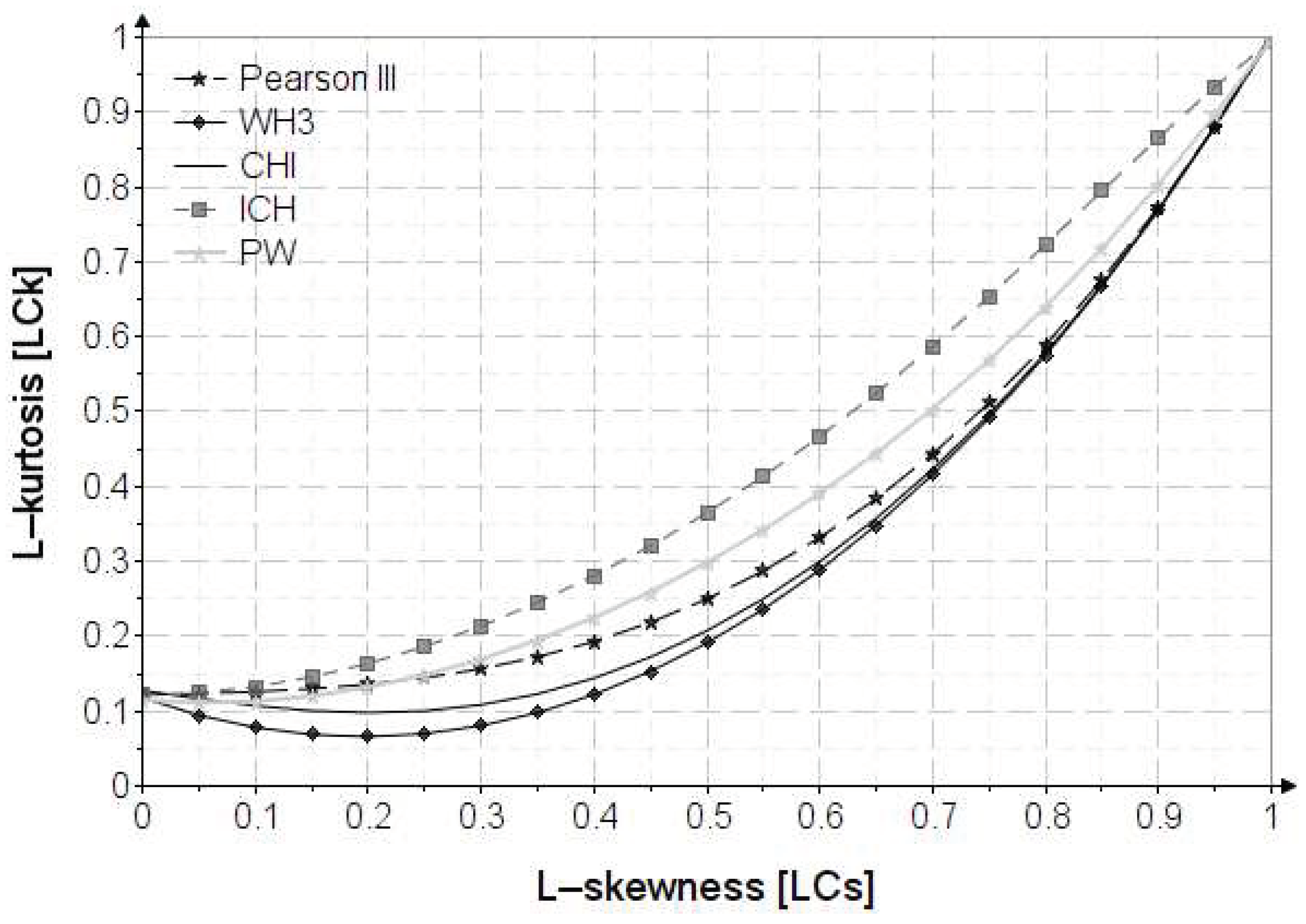
The best fit distribution for L-moments is based on the statistical indicator recommended by [8,13], the graph of variation between skewness and kurtosis obtained based on L-moments, presented in Appendix A.

The LSM corrects the

L_{1}

,

τ_{2}

and

τ_{3}

statistical parameters. In the system of equations,

τ_{3}

appears in the frequency factor through the shape parameter.

The solutions of the system are

L_{1}'

,

τ_{2}'

, and the corrected shape parameter, the latter determines the corrected

τ_{3}'

.

Solving the system of equations is done by numerical methods. The system of equations for the LSM is:

\frac{\partial}{\partial L_{1}} \sum_{i = 1}^{n} {(1 + K_{p} (p, α, . .) \cdot τ_{2} - \frac{x_{i}}{L_{1}})}^{2} = 0

(86)

\frac{\partial}{\partial τ_{2}} \sum_{i = 1}^{n} {(1 + K_{p} (p, α, . .) \cdot τ_{2} - \frac{x_{i}}{L_{1}})}^{2} = 0

(87)

\frac{\partial}{\partial α} \sum_{i = 1}^{n} {(1 + K_{p} (p, α, . .) \cdot τ_{2} - \frac{x_{i}}{L_{1}})}^{2} = 0

(88)

In the Kritski-Menkel case, where there are two parameters in the frequency factor, an additional equation appears.

The regionalization maps for the L-moments method with the corrected

τ_{2}'

and

τ_{3}'

can be made by applying the LSM to the data strings of the hydrometric stations.

The methodological approach regarding the determination of maximum flows is presented in Figure 4.

Application to hydrologic data

The case study consists in verifying the performances of this distributions through the statistical analysis of the maximum annual flows on the Ialomita River, Romania [11].

Ialomita River, code XI, is a part of the Danube hydrographic basin, located in the southern part of Romania, being its left tributary (Figure 5).

The main morphometric characteristics of the Ialomita river are presented in Table 4 [14].

The observed data are presented in Table 5, in descending order.

There are 33 annual records of flood, with the values of the main statistical indicators presented in Table 6.

where

μ, σ, C_{v}, C_{s}, C_{k}, L_{1}, L_{2}, L_{3}, L_{4}, τ_{2}, τ_{3}, τ_{4}

represent the mean, the standard deviation, the coefficient of variation, the skewness, the kurtosis, the four L-moments, the L-coefficient of variation, the L-skewness, respectively the L-kurtosis.

For parameter estimation with L-moments, the data series must be in ascending order for the calculation of natural estimators, respectively L-moments.

Results

The proposed methodology and distributions were applied to perform a statistical analysis of the maximum annual flows on the Ialomita river.

The distribution parameters were estimated for MOM, L-moments and LSM. For the MOM, the skewness coefficient was chosen depending on the origin of the flows according to Romanian regulations. Skewness is established based on some multiplication coefficients for

C_{v}

, chosen many times without reflecting the origin of the flows.

For the analyzed case study, the multiplication coefficient 2 applied to the coefficient of variation of the data string was used, resulting in a skewness of 1.054 different from 0.327 of the observed values.

In Table 7 are presented the results values of quantile distributions, for some of the most common exceedance probabilities in extreme values analysis.

Figure 6 and Figure 7, show the fitting distributions for annual minimum flow for Ialomita river. For plotting positions, the Landwehr formula was used.

Table 8 shows the values of the distributions parameters for the three methods of estimating.

The performance of the analyzed distribution is evaluated using the next two statistical measures [12]: Kiling-Gupta coefficient and Nash-Sutclif coefficient, presented as follows:

Nash Sutcliffe coefficient (E):

E = 1 - \frac{\sum_{i = 1}^{n} {(x_{i} - x (p_{i}))}^{2}}{{\sum_{i = 1}^{n} (x_{i} - μ_{x_{i}})}^{2}}

(89)

Kling-Gupta coefficient (KGE):

K G E = 1 - \sqrt{{(r - 1)}^{2} + {(\frac{σ_{x (p_{i})}}{σ_{x_{i}}} - 1)}^{2} + {(\frac{μ_{x (p_{i})}}{μ_{x_{i}}} - 1)}^{2}}

(90)

where

σ_{x_{i}}, μ_{x_{i}}, σ_{x (p_{i})}, μ_{x (p_{i})}

, represents standard deviation of observed values, mean of observed values, standard deviation of predicted value, mean of predicted value;

r

is the Pearson correlation coefficient:

r = \frac{\sum_{i = 1}^{n} (x_{i} - μ_{x_{i}}) \cdot (x (p_{i}) - μ_{x (p_{i})})}{\sqrt{{\sum_{i = 1}^{n} (x_{i} - μ_{x_{i}})}^{2} \cdot} \sqrt{\sum_{i = 1}^{n} {(x (p_{i}) - μ_{x (p_{i})})}^{2}}}

(91)

in which

x_{i}, μ_{x_{i}}, x (p_{i}), μ_{x (p_{i})}

, represents the observed values, mean of observed values, predicted value, average predicted value;

n

is the length of observed data.

The value of the coefficients E and KGE is between 1 and

- \infty

. The concordance criterion is represented by the value closest to the value 1. The distributions performance values are presented in Table 9.

Discutions

The distributions analyzed within the research of the Faculty of Hydrotechnics were exemplified in this article by the case study of the Ialomița river, Tăndărei section, presenting the results obtained for the two methods of estimating the parameters of the distributions and for the LSM of correcting the statistical parameters of the observed values.

The proposed methodology was applied to this case study because the Romanian regulation regarding the determination of maximum flows has this river as a case study, and the proposed methodology must be analyzed compared to the existing legislation.

Evaluation of the performance of distributions, the indicators Kling-Gupta coefficient and Nash-Sutcliff coefficient and

τ_{3} - τ_{4}

diagram were chosen, the latter with the disadvantage that it requires

n \geq 80

.

In Romania PE3 and KM are used for flood frequency analysis. Since the Gamma family distributions are frequently used in other countries as well, it was analyzed which of the distributions from this family give best results in the climatic and physiographic conditions in Romania. The method for estimating distribution parameters used in Romania is MOM.

Because the estimation of the parameters with MOM, the choice of the skewness coefficient is made by multiplying the

C_{v}

with a coefficient that reflects the origin of the flows, this methodology has the disadvantage that the choice does not always reflect this origin of the flows. Thus, it is proposed to achieve a regionalization regarding the maximum flows using the LSM method based on the statistical parameters estimated with the L-moments method, the latter being a method less influenced by the length of the data.

Another disadvantage of using the methodology by choosing the origin of flows is the fact that, in general, in Romania, the determination of maximum flows is based on the Pearson III transition coefficients with

C_{v} = 1

and

ξ = 4

only for relatively small hydrographic basins.

As can be seen from the results presented in table 8, the WH distribution has the best results, for both indicators. However, in the domain of low probabilities, this underestimates the maximum flows, preferring the PE3 and PW distributions, which are less sensitive to the length of the data. A possible disadvantage of the proposed distributions can be represented by the fact that their inverse functions are expressed using the inverse function of the Gamma distribution. However, this impediment is overcome by presenting the expression relations of the inverse function using the frequency factors, both for MOM and L-moments, and their approximation relations for the most used exceedance probabilities from the flood frequency analysis.

In Romania KM was an alternative for PE3 [16] but it is difficult to estimate the parameters. The PW distribution is a better alternative to PE3 than KM, having an inverse function similar to KM, but with the advantage that the frequency factor for MOM and L-moments depends on a single shape parameter. The presentation of the approximate forms of estimating the parameters and the frequency factors of the distribution, for the most common exceedance probabilities in hydrology, represents another advantage in choosing it as an alternative to KM.

The correction of the statistical parameters of the data observed from the case study, with LSM led to similar values for

L_{1}

, and

τ_{2}

, and the differences appear at

τ_{3}

, distinguishing three different value classes. The

τ_{3} - τ_{4}

diagram shows that for

τ_{3} \leq 0.5

, which is characteristic of Romania, the distribution closest to the parent (PE3) is PW.

Conclusions

This article presents a methodology for estimating maximum flows to replace the existing one which is outdated and a legacy from the USSR normative standards. The proposed methodology has the purpose of carrying out studies and regionalization of the maximum flows using the estimation of the parameters of the statistical distributions with the L-moments method calibrated with LSM. The calibration consists in obtaining some corrected statistical parameters of the observed values, following that through spatial interpolation and correlations depending on the physiographic characteristics, the regionalization of the maximum flows on the territory of Romania is obtained.

From the sampling analysis of the theoretical curves, it was observed that the stability of the curves is better for the parameter estimation with the L-moments method compared to the currently used method (MOM). The existing methodology leads to unrealistic maximum flow values. This approach leads to the overestimation of flows in the area of low exceedance probabilities, which lead to unsustainable costs for dams and the underestimation of flows for high exceedance probabilities, which are used for bankfull discharge channel.

Six distributions from the Gamma family were analyzed, with the PW distribution closest to PE3, the parent distribution. The PW distribution is an easy alternative to the KM distribution.

Approximation relationships of distribution parameters are presented, eliminating the need for iterative numerical calculation, in many cases this was an inconvenience in the application of certain probability distributions.

The frequency factor quantile expression for L-moments facilitated the application of distributions for regionalization studies, being presented and applied for the first time. An advantage is also the presentation of approximation relationships of the frequency factor for exceedance probabilities common in hydrology.

The future scope is the establishment of guidelines necessary for the realization of a robust, clear and concise normative regarding the regionalization of maximum flows using the L-moment estimation method. The final results of the research in the Faculty of Hydrotechnics will form the basis of a future material. [32,33].

All research was carried out by the authors in the Faculty of Hydrotechnics with data from hydrological studies in Romania.

Author Contributions

Conceptualization, C.I. and C.G.A.; methodology, C.I. and C.G.A.; software, C.I. and C.G.A.; validation, C.I. and C.G.A.; formal analysis, C.I. and C.G.A.; investigation, C.I. and C.G.A.; resources, C.I. and C.G.A.; data curation, C.I. and C.G.A.; writing—original draft preparation, C.I. and C.G.A.; writing—review and editing, C.I. and C.G.A.; visualization, C.I. and C.G.A.; supervision, C.I. and C.G.A.; project administration, C.I. and C.G.A.; funding acquisition, C.I. and C.G.A. All authors have read and agreed to the published version of the manuscript.

Funding

This research received no external funding.

Institutional Review Board Statement

Not applicable.

Informed Consent Statement

Not applicable.

Data Availability Statement

Not applicable.

Conflicts of Interest

The authors declare no conflicts of interest.

Abbreviations

MOM	the method of ordinary moments
L-moments	the method of linear moments
LSM	the method of Least squares
$μ$	expected value; arithmetic mean
$σ$	standard deviation
$C_{v}$	coefficient of variation
$C_{s}$	coefficient of skewness; skewness
$L_{1}, L_{2}, L_{3}$	linear moments
$τ_{2}, L C_{v}$	coefficient of variation based on the L-moments method
$τ_{3}, L C_{s}$	coefficient of skewness based on the L-moments method
$τ_{4}, L C_{k}$	coefficient of kurtosis based on the L-moments method
$ξ$	multiplication factor
PE3	Pearson III distribution
KM	Kristky - Menkel distribution
WH	Wilson-Hilferty distribution
CHI	three parameters CHI distribution
ICH	three parameters Inverse CHI distribution
PW	Pseudo Weibull distribution
INHGA	the National Institute of Hydrology and Water management

Appendix A. The variation of L-skewness-L-kurtosis

In the next section are presented the variation of L-kurtosis depending on the positive L-skewness, obtained with the L-moments method, for certain theoretical distributions often used in hydrology and in this article.

Figure 8. The variation diagram of

L C_{s} - L C_{k}

.

Figure 8. The variation diagram of

L C_{s} - L C_{k}

.

Pearson III:	$τ_{4} = 0 . 1217175 + 0 . 030285 \cdot τ_{3} + 0 . 0266125 \cdot τ_{3}^{2} + 0 . 8774691 \cdot τ_{3}^{3} - 0 . 0564795 \cdot τ_{3}^{4}$
Pearson V:	$τ_{4} = 0 . 1089545 - 0 . 1542626 \cdot τ_{3} + 1 . 0657605 \cdot τ_{3}^{2} - 0 . 3521005 \cdot τ_{3}^{3} + 0 . 3269967 \cdot τ_{3}^{4}$
Wilson-Hilferty:	$τ_{4} = 0 . 1177849 - 0 . 5367173 \cdot τ_{3} + 1 . 4180786 \cdot τ_{3}^{2} - 0 . 2084697 \cdot τ_{3}^{3} + 0 . 2098975 \cdot τ_{3}^{4}$
CHI:	$\begin{array}{l} τ_{4} = 0 . 1274475 - 0 . 2174617 \cdot τ_{3} - 0 . 0945508 \cdot τ_{3}^{2} + 2 . 6572905 \cdot τ_{3}^{3} - \\ 2 . 369862 \cdot τ_{3}^{4} + 0 . 9016064 \cdot τ_{3}^{5} \end{array}$
ICH:	$\begin{array}{l} τ_{4} = 0 . 1215494 + 0 . 0260015 \cdot τ_{3} + 0 . 6839989 \cdot τ_{3}^{2} + 2 . 3432188 \cdot τ_{3}^{3} - 7 . 9178585 \cdot τ_{3}^{4} + \\ 11 . 9165941 \cdot τ_{3}^{5} - 8 . 06007 \cdot τ_{3}^{6} + 1 . 8820702 \cdot τ_{3}^{7} \end{array}$
Pseudo-Weibull:	$τ_{4} = 0 . 1132189 - 0 . 1242052 \cdot τ_{3} + 1 . 1329458 \cdot τ_{3}^{2} - 0 . 4716246 \cdot τ_{3}^{3} + 0 . 3449906 \cdot τ_{3}^{4}$
Wakeby:	$τ_{4} = - 0.07347 + 0.14443 \cdot τ_{3} + 1.03879 \cdot τ_{3}^{2} - 0.14602 \cdot τ_{3}^{3} + 0.03357 \cdot τ_{3}^{4}$
Pareto:	$τ_{4} = - 0 . 0003668 + 0 . 2070484 \cdot τ_{3} + 0 . 9264 \cdot τ_{3}^{2} - 0 . 133564 \cdot τ_{3}^{3}$
GEV:	$τ_{4} = 0 . 1072214 + 0 . 1143838 \cdot τ_{3} + 0 . 8341466 \cdot τ_{3}^{2} - 0 . 0632425 \cdot τ_{3}^{3} + 0 . 0074607 \cdot τ_{3}^{4}$
Frechet:	$τ_{4} = 0 . 1069938 + 0 . 1155235 \cdot τ_{3} + 0 . 8294258 \cdot τ_{3}^{2} - 0 . 0528083 \cdot τ_{3}^{3}$
Weibull:	$τ_{4} = 0 . 1057425 - 0 . 0753465 \cdot τ_{3} + 0 . 6176919 \cdot τ_{3}^{2} + 0 . 5065127 \cdot τ_{3}^{3} - 0 . 1788008 \cdot τ_{3}^{4}$
LogNormal:	$τ_{4} = 0 . 1238145 - 0 . 032954 \cdot τ_{3} + 0 . 9783895 \cdot τ_{3}^{2} - 0 . 3929245 \cdot τ_{3}^{3} + 0 . 3174611 \cdot τ_{3}^{4}$
Log-Logistic:	$τ_{4} = \frac{1 + 5 \cdot τ_{3}^{2}}{6} ≃ 0.16667 + 0.83333 \cdot τ_{3}^{2}$
Paralogistic:	$τ_{4} = 0 . 1262814 + 0 . 0078207 \cdot τ_{3} + 0 . 9179335 \cdot τ_{3}^{2} - 0 . 0328508 \cdot τ_{3}^{3} - 0 . 0190348 \cdot τ_{3}^{4}$
Inverse Paralogistic:	$τ_{4} = 0 . 0577651 + 0 . 5568896 \cdot τ_{3} - 0 . 2198157 \cdot τ_{3}^{2} + 0 . 9069583 \cdot τ_{3}^{3} - 0 . 3025029 \cdot τ_{3}^{4}$

Appendix B. The frequency factors for the analyzed distributions

Table B1 shows the expressions of the frequency factors for MOM and L-moments.

Table B1. Frequency factors.

Distribution	Frequency factor, $K_{p} (p)$
	Quantile function (inverse function)
	Method of ordinary moments (MOM)	L-moments
	$x (p) = μ + σ \cdot K_{p} (p)$	$x (p) = L_{1} + L_{2} \cdot K_{p} (p)$
KM	$\frac{q g a m m a {(1 - p, α)}^{λ} - \frac{Γ (α + λ)}{Γ (α)}}{\sqrt{\frac{Γ (α + 2 \cdot λ)}{Γ (α)} - {(\frac{Γ (α + λ)}{Γ (α)})}^{2}}}$	$\frac{\frac{Γ (α)}{Γ (α + λ)} \cdot q g a m m a {(1 - p, α)}^{λ} - 1}{1 - \frac{2 \cdot Γ (α)}{Γ (α + λ)} \cdot \int_{0}^{1} q g a m m a {(1 - p, α)}^{λ} \cdot p \cdot d p}$
PE3	$\frac{q g a m m a (1 - p, α) - α}{\sqrt{α}}$	$\frac{\sqrt{π} \cdot Γ (α) (q g a m m a (1 - p, α) - α)}{Γ (α + 0.5)}$
WH	$\frac{q g a m m a {(1 - p, α)}^{\frac{1}{3}} - \frac{Γ (α + \frac{1}{3})}{Γ (α)}}{\sqrt{\frac{Γ (α + \frac{2}{3})}{Γ (α)} - \frac{Γ {(α + \frac{1}{3})}^{2}}{Γ {(α)}^{2}}}}$	$\frac{β}{L_{2}} \cdot (q g a m m a {(1 - p, α)}^{\frac{1}{3}} - \frac{Γ (α + \frac{1}{3})}{Γ (α)})$
CHI	$\frac{\sqrt{2} \cdot (Γ (\frac{α}{2}) \cdot \sqrt{q g a m m a (1 - p, \frac{α}{2})} - Γ (\frac{α + 1}{2}))}{Γ (\frac{α}{2}) \cdot \sqrt{α - 2 \cdot {(\frac{Γ (\frac{α + 1}{2})}{Γ (\frac{α}{2})})}^{2}}}$	$\frac{β}{L_{2}} \cdot (\sqrt{2 \cdot q g a m m a (1 - p, \frac{α}{2})} - \frac{\sqrt{2} \cdot Γ (\frac{α + 1}{2})}{Γ (\frac{α}{2})})$
ICH	$\frac{\frac{1}{\sqrt{q g a m m a (p, α)}} - \frac{Γ (α - 0.5)}{Γ (α)}}{\sqrt{\frac{Γ (α - 1)}{Γ (α)} - \frac{Γ {(α - 0.5)}^{2}}{Γ {(α)}^{2}}}}$	$\frac{β}{L_{2}} \cdot (\frac{1}{\sqrt{q g a m m a (p, α)}} - \frac{Γ (α - \frac{1}{2})}{Γ (α)})$
PW	$\frac{q g a m m a {(1 - p, \frac{1}{α} + 1)}^{\frac{1}{α}} - \frac{2^{\frac{2}{α} + 0.5} \cdot Γ (\frac{1}{α} + 0.5)}{\sqrt{2 \cdot π}}}{\sqrt{\frac{3^{\frac{3}{α} + 0.5} \cdot Γ (\frac{1}{α} + \frac{1}{3}) \cdot Γ (\frac{1}{α} + \frac{2}{3})}{2 \cdot π} - \frac{2^{\frac{4}{α}} \cdot Γ {(\frac{1}{α} + 0.5)}^{2}}{π}}}$	$\frac{β}{L_{2}} \cdot (q g a m m a (1 - p, \frac{1}{α} + 1) - \frac{2 \cdot Γ (\frac{2}{α})}{Γ (\frac{1}{α})})$

Appendix C. Estimation of the frequency factor for the PE3 distribution

The frequency factor, for MOM, can be estimated using a polynomial function:

K_{p} (p) = a + b \cdot C_{s} + c \cdot C_{s}^{2} + d \cdot C_{s}^{3} + e \cdot C_{s}^{4} + f \cdot C_{s}^{5} + g \cdot C_{s}^{6} + h \cdot C_{s}^{7}

Table C1. The frequency factor for estimation with MOM.

P [%]	a	b	c	d	e	f	g	h
0.01	3.71828	2.146200	1.55790E-01	-7.69315E-02	1.50378E-02	-1.72710E-03	1.1060E-04	-3.033E-06
0.1	3.09014	1.426290	4.96310E-02	-4.21189E-02	7.94983E-03	-8.33091E-04	4.7935E-05	-1.179E-06
0.5	2.57601	0.937811	-4.85114E-03	-2.43670E-02	4.59158E-03	-4.29197E-04	2.0466E-05	-3.82E-07
1	2.32661	0.733146	-2.18707E-02	-1.85502E-02	3.58677E-03	-3.15387E-04	1.3017E-05	-1.71E-07
2	2.05408	0.533496	-3.42010E-02	-1.38703E-02	2.86305E-03	-2.39574E-04	8.3060E-06	-4.17E-08
3	1.88115	0.419782	-3.89303E-02	-1.16643E-02	2.57668E-03	-2.13746E-04	6.8730E-06	-5.63E-09
5	1.64524	0.280836	-4.18754E-02	-9.45489E-03	2.37315E-03	-2.02670E-04	6.5730E-06	-4.92E-09
10	1.28196	0.103328	-3.95043E-02	-7.48248E-03	2.41382E-03	-2.31322E-04	8.9870E-06	-8.238E-08
20	0.842052	-0.0526706	-2.7535E-02	-6.8667E-03	2.9690E-03	-3.3372E-04	1.4454E-05	-1.620E-07
40	0.254237	-0.164334	7.0463E-03	-1.5678E-02	7.8439E-03	-1.3773E-03	1.0621E-04	-3.076E-06
50	0.0006921	-0.174131	1.9451E-02	-1.8001E-02	1.0156E-02	-2.0960E-03	1.8921E-04	-6.3925E-06
80	-0.845883	-0.0108923	-4.1893E-02	6.4938E-02	-2.2096E-02	3.3839E-03	-2.4937E-04	7.203E-06

The frequency factor, for L-moments, can be estimated using a polynomial function:

K_{p} (p) = a + b \cdot τ_{3} + c \cdot τ_{3}^{2} + d \cdot τ_{3}^{3}

Table C2. The frequency factor for estimation with L-moments.

P [%]	a	b	c	d
0.01	6.5901E+00	2.3380E+01	1.7214E+01	-3.7117E+00
0.1	5.4765E+00	1.5559E+01	8.9860E+00	4.7591E-01
0.5	4.5651E+00	1.0245E+01	4.4167E+00	1.5525E+00
1	4.1231E+00	8.0174E+00	2.8187E+00	1.5366E+00
2	3.6401E+00	5.8441E+00	1.4754E+00	1.2797E+00
3	3.3336E+00	4.6063E+00	8.1958E-01	1.0420E+00
5	2.9154E+00	3.0940E+00	1.4699E-01	6.6702E-01
10	2.2715E+00	1.1625E+00	-4.5319E-01	8.2415E-02
20	1.4918E+00	-5.3214E-01	-6.3128E-01	-3.9305E-01
40	4.4907E-01	-1.6990E+00	-2.5238E-01	-4.9031E-01
50	4.4000E-06	-1.8140E+00	4.2269E-03	-2.8014E-01
80	-1.4918E+00	-5.2533E-01	6.2038E-01	9.2798E-01
90	-2.2715E+00	1.1681E+00	4.4733E-01	1.1400E+00

Appendix D. Estimation of the frequency factor for the PW distribution

The frequency factor, for MOM, can be estimated using a polynomial function:

K_{p} (p) = a + b \cdot C_{s} + c \cdot C_{s}^{2} + d \cdot C_{s}^{3} + e \cdot C_{s}^{4} + f \cdot C_{s}^{5}

Table D1. The frequency factor for estimation with MOM.

P [%]	a	b	c	d	e	f
0.01	3.4996E+00	1.5864E+00	8.6821E-01	-2.3732E-01	2.5030E-02	-9.7960E-04
0.1	2.9199E+00	1.3301E+00	3.0426E-01	-1.2436E-01	1.5293E-02	-6.5680E-04
0.5	2.4562E+00	1.0397E+00	8.5597E-03	-4.6888E-02	7.2443E-03	-3.4540E-04
1	2.2328E+00	8.8003E-01	-8.1686E-02	-1.7965E-02	3.9244E-03	-2.0810E-04
2	1.9883E+00	6.9793E-01	-1.4374E-01	6.1815E-03	9.4670E-04	-7.9600E-05
3	1.8324E+00	5.8099E-01	-1.6511E-01	1.7381E-02	-5.4670E-04	-1.2400E-05
5	1.6181E+00	4.2340E-01	-1.7444E-01	2.7637E-02	-2.0649E-03	5.9200E-05
10	1.2825E+00	1.9499E-01	-1.5223E-01	3.3044E-02	-3.2535E-03	1.2290E-04
20	8.6399E-01	-3.6722E-02	-8.5717E-02	2.6066E-02	-3.0572E-03	1.2980E-04
40	2.7955E-01	-2.2427E-01	2.3522E-02	3.8173E-03	-9.5000E-04	5.2600E-05
50	1.9272E-02	-2.5020E-01	6.3046E-02	-6.6079E-03	2.1180E-04	4.6000E-06
80	-8.6666E-01	-6.9671E-02	9.8113E-02	-2.5802E-02	2.8927E-03	-1.2040E-04
90	-1.3247E+00	1.7748E-01	3.9823E-02	-1.9393E-02	2.6296E-03	-1.2090E-04

The frequency factor, for L-moments, can be estimated using a polynomial function:

K_{p} (p) = a + b \cdot τ_{3} + c \cdot τ_{3}^{2} + d \cdot τ_{3}^{3}

Table D2. The frequency factor for estimation with L-moments.

P [%]	a	b	c	d
0.01	6.1892E+00	1.7503E+01	2.7734E+01	8.7400E+01
0.1	5.2382E+00	1.2376E+01	1.8193E+01	3.7067E+01
0.5	4.4311E+00	8.6236E+00	1.1153E+01	1.2622E+01
1	4.0301E+00	6.9597E+00	8.1540E+00	5.2011E+00
2	3.5848E+00	5.2680E+00	5.2722E+00	-1.8468E-01
3	3.2983E+00	4.2675E+00	3.6844E+00	-2.3498E+00
5	2.9026E+00	3.0001E+00	1.8468E+00	-4.0126E+00
10	2.2826E+00	1.2872E+00	-1.9313E-01	-4.3663E+00
20	1.5151E+00	-3.5053E-01	-1.3496E+00	-2.7006E+00
40	4.6429E-01	-1.6574E+00	-8.8083E-01	1.3155E-01
50	5.3035E-03	-1.8582E+00	-1.7379E-01	8.4985E-01
80	-1.5241E+00	-6.6641E-01	2.0718E+00	6.9287E-02
90	-2.3051E+00	1.2100E+00	1.3526E+00	-6.2836E-01

Appendix E. Estimation of the frequency factor for the WH distribution

The frequency factor, for MOM, can be estimated using a polynomial function:

K_{p} (p) = a + b \cdot C_{s} + c \cdot C_{s}^{2} + d \cdot C_{s}^{3} + e \cdot C_{s}^{4} + f \cdot C_{s}^{5} + g \cdot C_{s}^{6} + h \cdot C_{s}^{7}

Table E1. The frequency factor for estimation with MOM.

P [%]	a	b	c	d	e	f	g	h
0.01	3.6510405	0.2505395	0.7676395	- 0.2464009	0.0512864	- 0.0067085	0.0004888	- 0.000015
0.1	3.0545055	0.3000583	0.5675829	- 0.1826804	0.0359966	- 0.0044818	0.0003147	- 0.0000094
0.5	2.5588885	0.3077142	0.4177707	- 0.1419139	0.0264387	- 0.0031008	0.0002072	- 0.0000059
1	2.3161851	0.2995336	0.3494063	- 0.1261503	0.0227822	- 0.0025723	0.0001664	- 0.0000047
2	2.0493565	0.2811829	0.2776375	- 0.1120499	0.0195234	- 0.0020986	0.0001322	- 0.0000036
3	1.8791548	0.2649262	0.2323711	- 0.1038466	0.0174799	- 0.0017770	0.0001113	- 0.0000032
5	1.6454272	0.2412568	0.1614119	- 0.0851039	0.0109925	- 0.0004410	- 0.0000055	0.0000004
10	1.2876723	0.1587243	0.1123855	- 0.0984686	0.0124264	0.0010469	- 0.0002802	0.0000137
20	0.8568022	- 0.0261822	0.2459759	- 0.3251841	0.1209999	- 0.0204256	0.0016521	- 0.0000522
40	0.221592	0.2283007	- 0.6972333	0.3479014	- 0.0756093	0.0080699	- 0.0003912	0.0000058
50	- 0.0234312	0.1284028	- 0.7683876	0.5215176	- 0.1544872	0.0236166	- 0.001829	0.0000569
80	- 0.8056988	- 0.5881204	0.7109393	- 0.2807399	0.0555428	- 0.0058035	0.0002953	- 0.0000053
90	- 1.2747028	- 0.3048433	0.9443876	- 0.5464102	0.1534292	- 0.0232169	0.0018152	- 0.0000575

The frequency factor, for L-moments, can be estimated using a polynomial function:

K_{p} (p) = a + b \cdot τ_{3} + c \cdot τ_{3}^{2} + d \cdot τ_{3}^{3}

Table E2. The frequency factor for estimation with L-moments.

P [%]	a	b	c	d
0.01	6.4509E+00	1.9071E+00	4.1617E+01	-1.0532E+02
0.1	5.4003E+00	2.6569E+00	2.6320E+01	-6.0802E+01
0.5	4.5263E+00	2.8800E+00	1.6160E+01	-3.2938E+01
1	4.0979E+00	2.8467E+00	1.2038E+01	-2.2373E+01
2	3.6266E+00	2.6984E+00	8.1403E+00	-1.3072E+01
3	3.3260E+00	2.5422E+00	5.9927E+00	-8.3770E+00
5	2.9141E+00	2.2514E+00	3.4594E+00	-3.4404E+00
10	2.2759E+00	1.6342E+00	4.1013E-01	1.0766E+00
20	1.4978E+00	6.4805E-01	-2.0137E+00	2.5104E+00
40	4.5153E-01	-8.8689E-01	-3.1967E+00	1.8128E+00
50	-8.8000E-05	-1.5121E+00	-2.8183E+00	2.4211E+00
80	-1.4975E+00	-2.2811E+00	6.5256E+00	-1.7016E+00
90	-2.2759E+00	-6.8892E-01	1.5925E+01	-3.1219E+01

Appendix F. Estimation of the frequency factor for the CHI distribution

The frequency factor, for MOM, can be estimated using a polynomial function:

K_{p} (p) = a + b \cdot C_{s} + c \cdot C_{s}^{2} + d \cdot C_{s}^{3} + e \cdot C_{s}^{4} + f \cdot C_{s}^{5} + g \cdot C_{s}^{6} + h \cdot C_{s}^{7}

Table F1. The frequency factor for estimation with MOM.

P [%]	a	b	c	d	e	f	g	h
0.01	3.8180365	1.2940979	-0.0921369	0.1793798	-0.0663766	0.0113496	-0.0009526	0.0000317
0.1	3.1506027	0.9297019	0.0097711	0.0854903	-0.0376125	0.0068066	-0.0005868	0.0000198
0.5	2.6120951	0.6514242	0.0705661	0.0190737	-0.0171001	0.0035688	-0.0003263	0.0000114
1	2.3532411	0.5253934	0.0912867	-0.0090844	-0.0083033	0.0021816	-0.0002148	0.0000078
2	2.0720383	0.3959552	0.1067083	-0.0364377	0.0003724	0.0008178	-0.0001049	0.0000042
3	1.8944635	0.3189768	0.1123408	-0.0517504	0.005335	0.000044	-0.0000422	0.0000021
5	1.6530963	0.2219528	0.113368	-0.0688344	0.0109944	-0.0007973	0.0000254	-0.0000002
10	1.2833294	0.092811	0.0982755	-0.0830704	0.0152487	-0.0009201	-0.000008	0.0000019
20	0.8506717	-0.1081478	0.2126606	-0.2104821	0.0669975	-0.009839	0.0006949	-0.0000192
40	0.2198563	0.0387651	-0.2445912	0.0445053	0.0167409	-0.0063776	0.0007446	-0.0000299
50	-0.0495036	0.1528366	-0.5577415	0.3104498	-0.0757608	0.0094393	-0.0005846	0.0000141
80	-0.7928764	-0.3107709	0.2053254	0.0291907	-0.0367498	0.0087558	-0.0008757	0.0000325
90	-1.2094798	-0.3843972	0.7941788	-0.3843311	0.0923544	-0.0121178	0.0008302	-0.0000233

The frequency factor, for L-moments, can be estimated using a polynomial function:

K_{p} (p) = a + b \cdot τ_{3} + c \cdot τ_{3}^{2} + d \cdot τ_{3}^{3}

Table F2. The frequency factor for estimation with L-moments.

P [%]	a	b	c	d
0.01	6.6340E+00	2.0104E+01	-8.2733E+01	2.9055E+02
0.1	5.4994E+00	1.3934E+01	-4.8112E+01	1.6946E+02
0.5	4.5769E+00	9.4634E+00	-2.5980E+01	9.2610E+01
1	4.1311E+00	7.5119E+00	-1.7365E+01	6.2699E+01
2	3.6449E+00	5.5593E+00	-9.5834E+00	3.5580E+01
3	3.3369E+00	4.4238E+00	-5.5300E+00	2.1350E+01
5	2.9172E+00	3.0116E+00	-1.0878E+00	5.5510E+00
10	2.2719E+00	1.1633E+00	3.3838E+00	-1.0973E+01
20	1.4915E+00	-5.0748E-01	5.2537E+00	-1.9221E+01
40	4.4887E-01	-1.6942E+00	2.8105E+00	-1.2662E+01
50	-1.3200E-04	-1.8160E+00	5.4992E-01	-4.6652E+00
80	-1.4923E+00	-4.8443E-01	-7.3019E+00	3.2222E+01
90	-2.2723E+00	1.2407E+00	-7.0520E+00	3.9498E+01

Appendix G. Built-in function in Mathcad and Excel

Γ (x)

-returns the value of the Euler gamma function of x;

Γ (α, x)

-returns the value of the incomplete gamma function of x with parameter a;

d g a m m a (x, s)

-returns the probability density for value x, for Gamma distribution;

p g a m m a (x, s)

-returns the cumulative probability distribution for value x, for Gamma distribution;

q g a m m a (p, s)

-returns the inverse cumulative probability distribution for probability p, for Gamma distribution. This can also be found in other dedicated programs (the GAMMA.INV function in Excel).

q n o r m (p, 0, 1)

-returns the inverse standard cumulative probability distribution for probability p, for Normal distribution, (NORM.INV function in Excel).

p l n o r m (x, α, β)

-returns the cumulative probability distribution for value x, for LogNormal distribution;

q l n o r m (p, μ, σ)

-returns the inverse cumulative probability distribution for probability p, for LogNormal distribution, (LOGNORM.INV function in Excel).

e r f (x)

-returns the error function;

References

Teodorescu, I.; Filotti, A.; Chiriac, V.; Ceausescu, V.; Florescu, A. Water management; Ceres Publishing House: Bucharest, Romania, 1973. [Google Scholar]
Popovici, A. Dams for water accumulations, vol.II; Technical Publishing House: Bucharest, Romania, 2002. [Google Scholar]
Alina-Ioana Popescu-Busan et al 2019 IOP Conf. Ser.: Mater. Sci. Eng. 471 102049.
Carrillo, V.; Petrie, J.; Timbe, L.; Pacheco, E.; Astudillo, W.; Padilla, C.; Cisneros, F. Validation of an Experimental Procedure to Determine Bedload Transport Rates in Steep Channels with Coarse Sediment. Water 2021, 13, 672. [Google Scholar] [CrossRef]
Bulletin 17B Guidelines for determining Flood Flow Frequency; Hydrology Subcommittee, Interagency Advisory Committee on Water Data, U.S. Department of the Interior, U.S. Geological Survey, office of Water Data Coordination, Reston, Virginia: 1981.
Bulletin 17C Guidelines for determining Flood Flow Frequency; U.S. Department of the Interior, U.S. Geological Survey, Reston, Virginia: 2017.
Hosking, J.R.M. L-moments: Analysis and Estimation of Distributions using Linear, Combinations of Order Statistics. J. R. Statist. Soc. 1990, 52, 105–124. [Google Scholar] [CrossRef]
Hosking, J.R.M; Wallis, J.R. Regional Frequency Analysis, An Approach based on L-moments. Cambridge University Press, the Edinburgh Building, Cambridge CB2 2RU, UK: 1997; ISBN 13 978-0-521-43045-6.
Nipada Papukdee, Jeong-Soo Park & Piyapatr Busababodhin (2022) Penalized likelihood approach for the four-parameter kappa distribution, Journal of Applied Statistics, 49:6, 1559-1573. [CrossRef]
Yire Shin, Jeong-Soo Park, Modeling climate extremes using the four-parameter kappa distribution for r-largest order statistics, Weather and Climate Extremes, Volume 39, 2023, 100533, ISSN 2212-0947. [CrossRef]
The Regulations Regarding the Establishment of Maximum Flows and Volumes for the Calculation of Hydrotechnical Retention Constructions; Indicative NP 129-2011; Ministry of Regional Development and Tourism: Bucharest, Romania, 2012.
Mohamedmaroof P. Shaikh, Sanjaykumar M. Yadav, Vivek L. Manekar; Assessment of the empirical methods for the development of the synthetic unit hydrograph: a case study of a semi-arid river basin. Water Practice and Technology 1 January 2022; 17 (1): 139–156. [CrossRef]
Rao, A.R.; Hamed, K.H. Flood Frequency Analysis; CRC Press LLC: Boca Raton, FL, USA, 2000. [Google Scholar]
Ilinca, C.; Anghel, C.G. Flood-Frequency Analysis for Dams in Romania. Water 2022, 14, 2884. [Google Scholar] [CrossRef]
Constantinescu, M.; Golstein, M.; Haram, V.; Solomon, S. Hydrology; Technical Publishing House: Bucharest, Romania, 1956. [Google Scholar]
STAS 4068/1-82; Maximum Water Discharges and Volumes, Determination of maximum Water Discharges and Volumes of Watercourses, the Romanian standardization institute, Romania.
Diaconu, C.; Serban, P. Syntheses and hydrological regionalization; Technical Publishing House: Bucharest, Romania, 1994. [Google Scholar]
Matalas, N.C. Probability Distribution of Low Flows. Statistical Studies in Hydrology. Geological Survey, United States Government Printing Office, USA, Washington:1963.
Crooks, G.E. Field Guide To Continuous Probability Distributions, Berkeley Institute for Theoretical Science: Berkeley, California, United States, v.1.0.0, 2019.
Nascimento, Fernando & Bourguignon, Marcelo & Leão, Jeremias. (2015). Extended generalized extreme value distribution with applications in environmental data. Hacettepe University Bulletin of Natural Sciences and Engineering Series B: Mathematics and Statistics. [CrossRef]
Song, S.; Kang, Y.; Song, X.; Singh, V.P. MLE-Based Parameter Estimation for Four-Parameter Exponential Gamma Distribution and Asymptotic Variance of Its Quantiles. Water 2021, 13, 2092. [Google Scholar] [CrossRef]
Ashkar, F., Bobée, B., Leroux, D. et al. The generalized method of moments as applied to the generalized gamma distribution. Stochastic Hydrol Hydraul 2, 161–174 (1988). [CrossRef]
Abramowitz, Milton; Stegun, Irene Ann, eds. (1983). Handbook of Mathematical Functions with Formulas, Graphs, and Mathematical Tables. Applied Mathematics Series. Vol. 55. Washington D.C.; New York: United States Department of Commerce, National Bureau of Standards; Dover Publications. ISBN 978-0-486-61272-0. LCCN 64-60036. MR 0167642. LCCN 65-12253.
Anghel, C.G.; Ilinca, C. Parameter Estimation for Some Probability Distributions Used in Hydrology. Appl. Sci. 2022, 12, 12588. [Google Scholar] [CrossRef]
TEFARUK HAKTANIR (1991) Statistical modelling of annual maximum flows in Turkish rivers, Hydrological Sciences Journal, 36:4, 367-389. [CrossRef]
V. Gh. Voda: New Statistical Models in Durability Analysis (in Romanian). Academy Publ. House, Bucharest 1980.
Gubareva, T.S.; Gartsman, B.I. Estimating Distribution Parameters of Extreme Hydrometeorological Characteristics by L-Moment Method. Water Resour. 2010, 37, 437–445. [Google Scholar] [CrossRef]
Singh, V.P. Entropy-Based Parameter Estimation in Hydrology; Springer Science + Business Media: Dordrecht, The Netherlands, 1998; ISBN 978-90-481-5089-2, ISBN 978-94-017-1431-0 (eBook). [CrossRef]
Citakoglu, Hatice & Demir, Vahdettin & Haktanir, Tefaruk. (2017). L−MOMENTLER YÖNTEMİYLE KARADENİZ'E DÖKÜLEN AKARSULARA AİT YILLIK ANLIK MAKSİMUM AKIM DEĞERLERİNİN BÖLGESEL FREKANS ANALİZİ. Ömer Halisdemir Üniversitesi Mühendislik Bilimleri Dergisi. 6. 571-580. [CrossRef]
World Meteorological Organization. (WMO-No.718) 1989 Statistical Distributions for Flood Frequency Analysis; Operational Hydrology Report no. 33; WHO: Geneva, Switzerland, 1989. [Google Scholar]
STAS 4068/1962; Maximum Water Discharges and Volumes, Determination of maximum Water Discharges and Volumes of Watercourses, the Romanian standardization institute, Romania.
IRINA, GOIA & STEFANIA, IGRET & VIRGIL, MARINAS & ALEXANDRA, OLARIU & MONICA, ROMAN. (2022). Internships, Skills and Employability: Mapping the Field through a Bibliometric Analysis. ECONOMIC COMPUTATION AND ECONOMIC CYBERNETICS STUDIES AND RESEARCH. 56. 331-348. [CrossRef]
Stefan Ciprian Stanca et al 2023 IOP Conf. Ser.: Earth Environ. Sci. 1136 012032.

Figure 1. Cases of the inverse function for the analyzed Gamma family distributions.

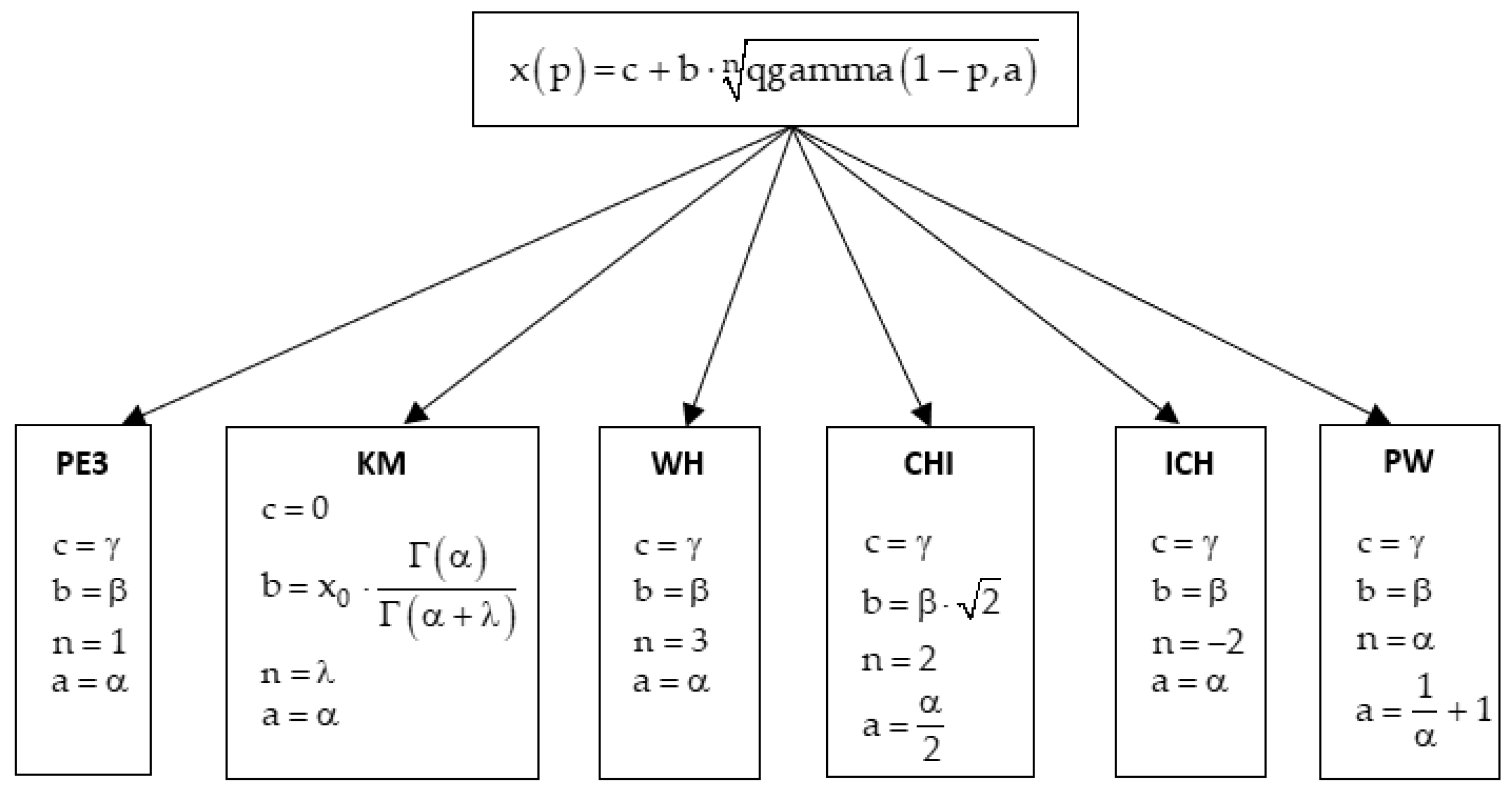
Figure 2. Theoretical and sample curves for PW and PE3.

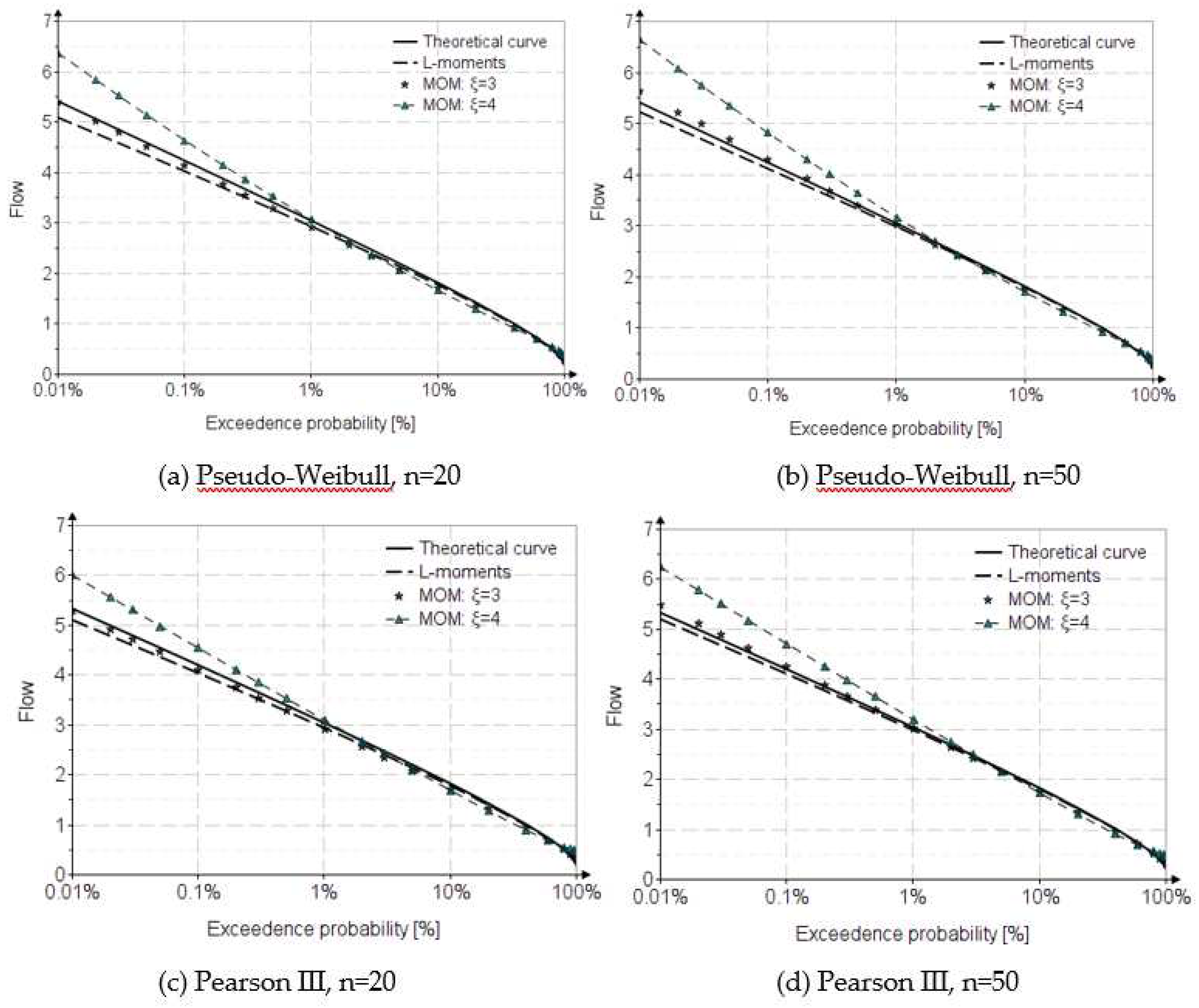
Figure 3. The theoretical curve PE3 and the curves from the INHGA methodology.

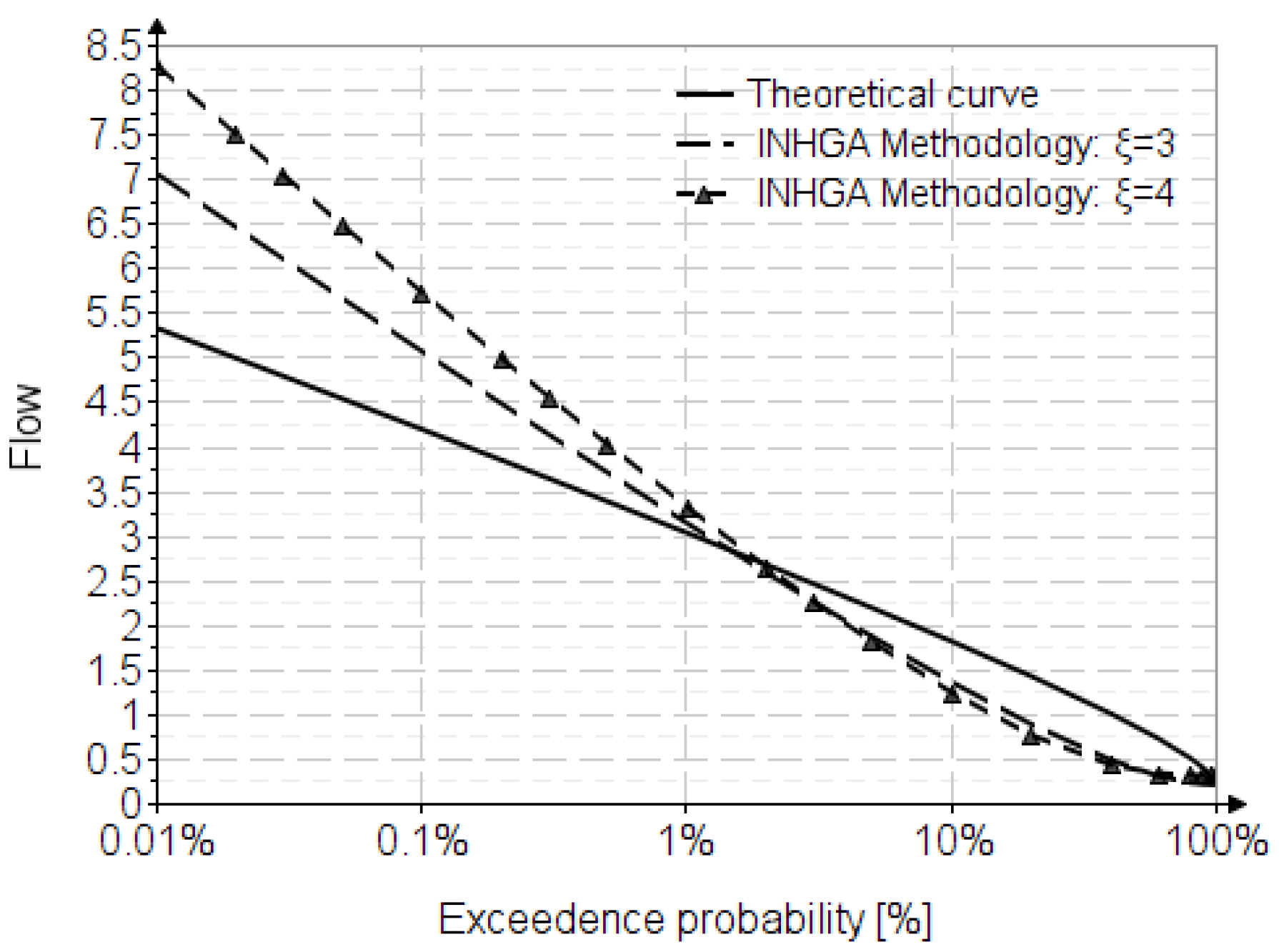
Figure 4. Methodological approach.

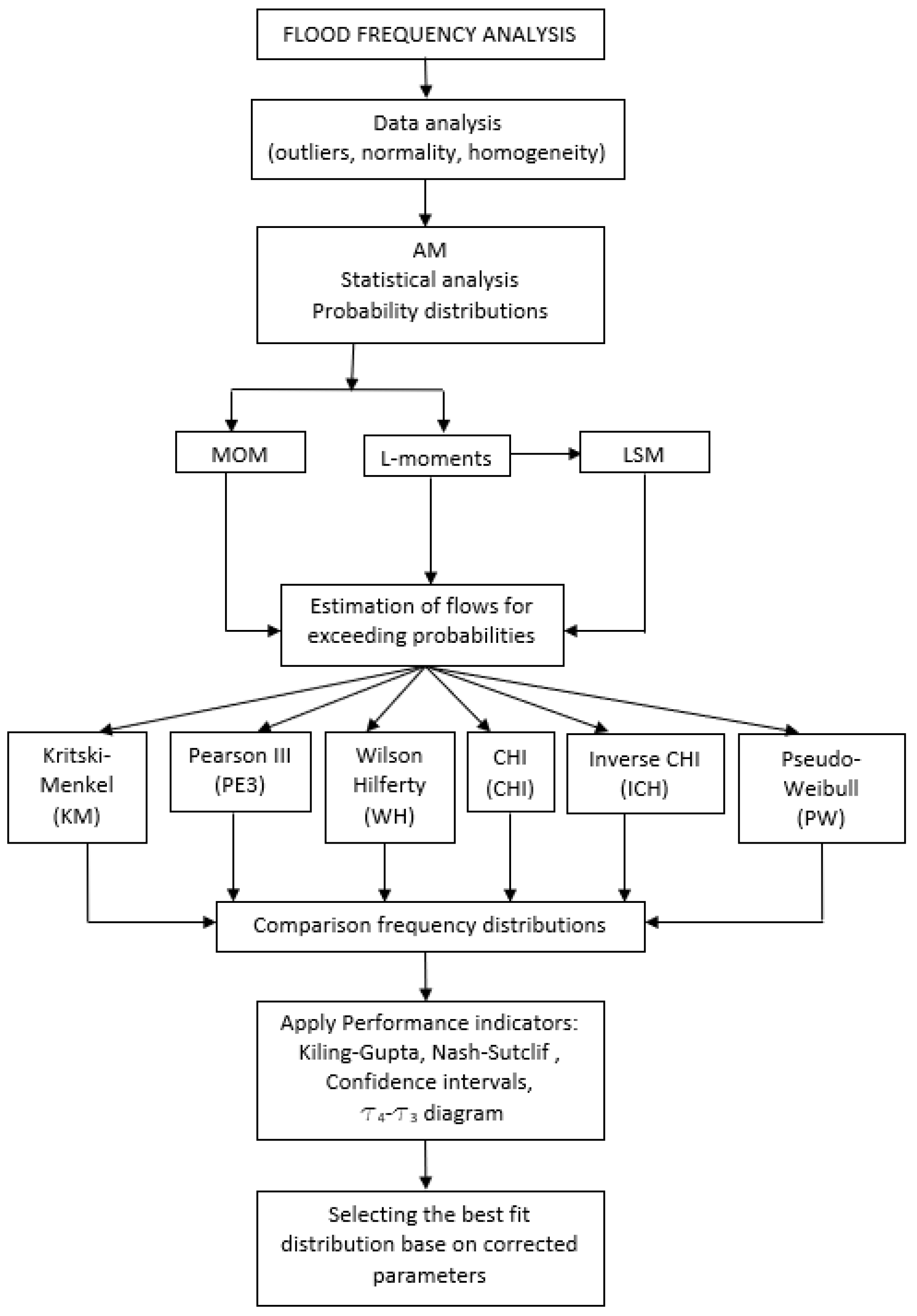
Figure 5. The Ialomita river location – Tandarei hydrometric station.

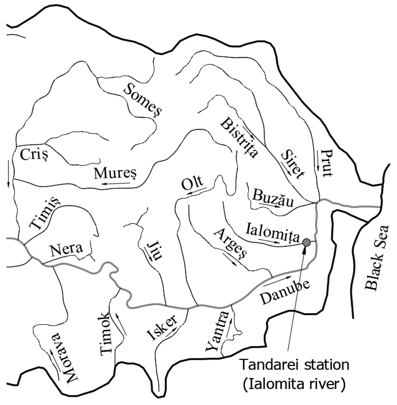
Figure 6. Fitting distributions.

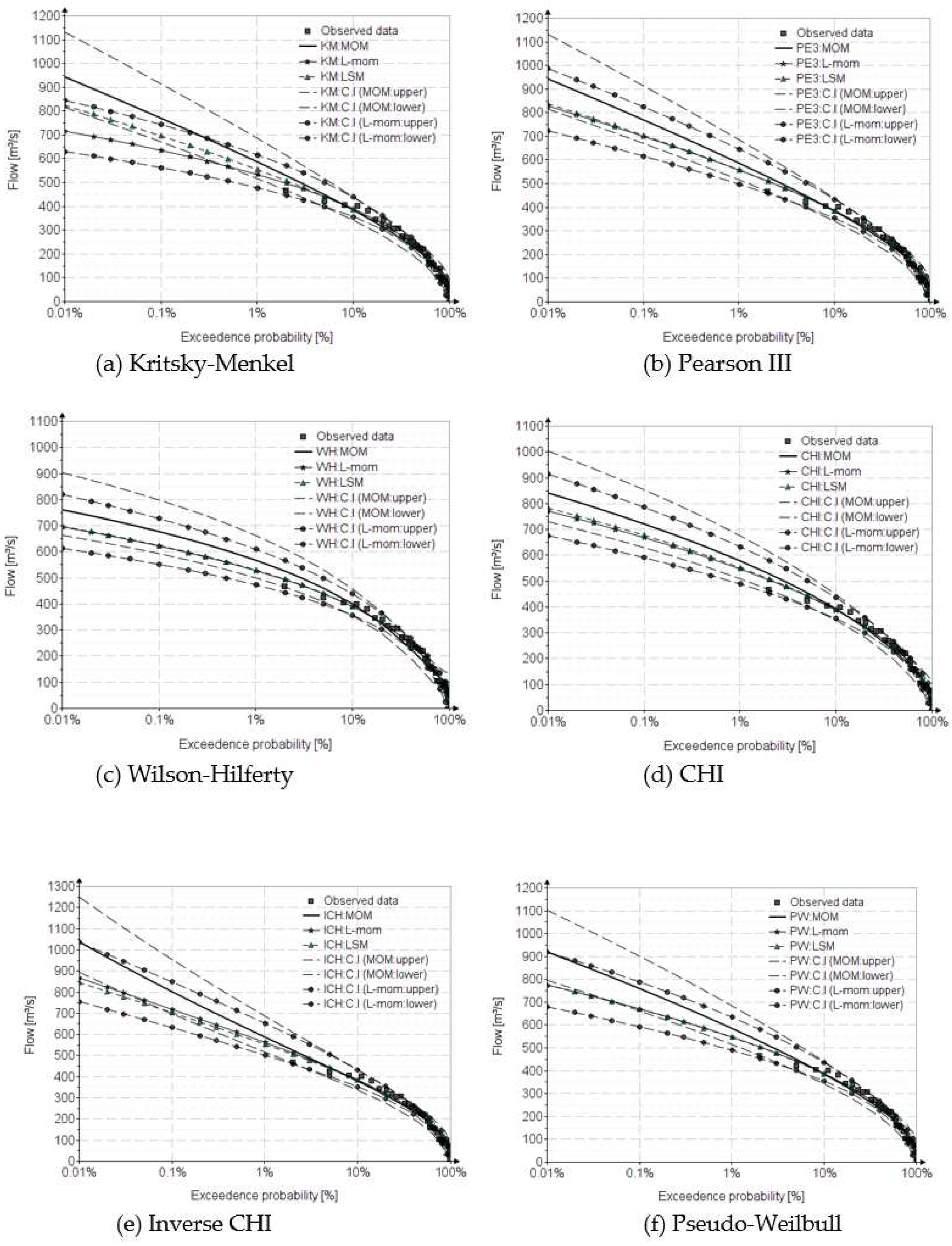
Figure 7. Comparison for estimation with MOM, L-moments and LSM.

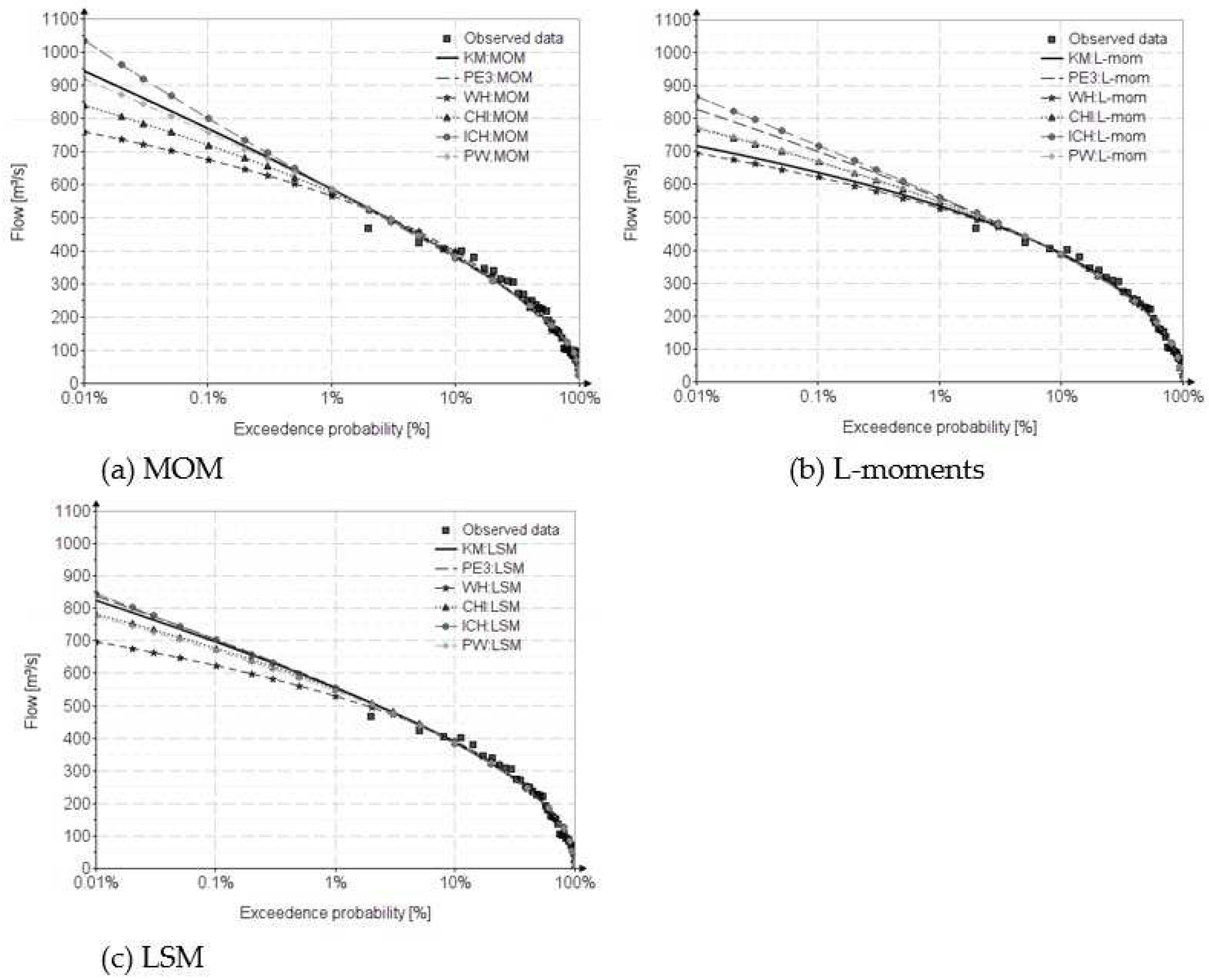
Table 1. Novelty elements.

A. Distribution	New Elements
KM, WH, CHI, ICH, PW	inverse function; exact and approximate relation for the parameter estimation with the MOM and L-moments method
B. Frequency factors	Frequency factors for PEIII, KM, WH, CHI, ICH, PW
C. Expressing the quantile function using the frequency factor for L-moments	quantile function using the frequency factor for L-moments for PEIII, KM, WH, CHI, ICH, PW
D. Approximate relations for estimating the frequency factors	for PEIII, PW, WH, CHI
E. Method of calibrating statistical indicators obtained with L-moments	For all distributions using Least Square Method (LSM)
F. Raw and central moments up to 6 order	PEIII, KM

Table 2. Statistical parameters.

Statistical parameters		Quantitative measures
MOM	L-moments	Quantitative measures
$μ = m_{1}$	$L_{1} = μ$	Expected value (Kritsky-Menkel (KMarithmetic mean)
$C_{v} = \frac{\sqrt{m_{2}}}{m_{1}} = \frac{σ}{μ}$	$τ_{2} = \frac{L_{2}}{L_{1}}$	Coefficient of variation/L-coefficient of variation
$C_{s} = \frac{m_{3}}{m_{2}^{1.5}}$	$τ_{3} = \frac{L_{3}}{L_{2}}$	Skewness/L-skewness
$C_{s c} = ξ \cdot C_{v}$	$τ_{3} = \frac{L_{3}}{L_{2}}$	Skewness chosen in Romania

Table 3. Theoretical curve sampling results.

	Sampling						Theoretical analytical curve
Statistical parameters	MOM			L-moments			MOM	L-moments
Statistical parameters	20	30	50	20	30	50	MOM	L-moments
PSEUDO-WEIBULL
$μ / L_{1}$	0.970	0.979	0.986	0.970	0.979	0.986	1	1
$C_{v} / τ_{2}$	0.582	0.586	0.592	0.326	0.324	0.322	0.609	0.320
$C_{s} / τ_{3}$	1.049	1.126	1.210	0.234	0.238	0.241	1.527	0.250
PEARSON III
$μ / L_{1}$	0.970	0.979	0.987	0.970	0.979	0.987	1	1
$C_{v} / τ_{2}$	0.582	0.586	0.592	0.326	0.324	0.322	0.608	0.320
$C_{s} / τ_{3}$	1.046	1.121	1.202	0.235	0.238	0.242	1.505	0.250

Table 4. The morphometric characteristics.

Length [km]	Average stream slope [‰]	Sinuosity coefficient [-]	Average altitude, [m]	Drainage area, [km²]
417	15	1.88	327	10350

Table 5. The observed data from Tandarei hydrometric station.

		1	2	3	4	5	6	7	8	9	10	11
Flow	[m³/s]	468	424	405	401	381	346	341	317	308	306	273
		12	13	14	15	16	17	18	19	20	21	22
Flow	[m³/s]	270	251	249	237	228	224	220	192	180	161	159
		23	24	25	26	27	28	29	30	31	32	33
Flow	[m³/s]	152	136	106	104	103	94.5	89.0	85.0	72.0	65.3	47.5

Table 6. The statistical indicators of the observed values.

$μ$	$σ$	$C_{v}$	$C_{s}$	$C_{k}$	$L_{1}$	$L_{2}$	$L_{3}$	$L_{4}$	$τ_{2}$	$τ_{3}$	$τ_{4}$
[m³/s]	[m³/s]	[-]	[-]	[-]	[m³/s]	[m³/s]	[m³/s]	[m³/s]	[-]	[-]	[-]
224.1	118	0.527	0.327	2.074	224.1	68.6	6.13	1.69	0.306	0.089	0.025

Table 7. Quantile results of the analyzed distributions.

P	The analyzed distributions
P	KM			PE3			WH			CHI			ICH			PW
[%]	MOM	L-mom	LSM	MOM	L-mom	LSM	MOM	L-mom	LSM	MOM	L-mom	LSM	MOM	L-mom	LSM	MOM	L-mom	LSM
[%]	[m³/s]	[m³/s]	[m³/s]	[m³/s]	[m³/s]	[m³/s]	[m³/s]	[m³/s]	[m³/s]	[m³/s]	[m³/s]	[m³/s]	[m³/s]	[m³/s]	[m³/s]	[m³/s]	[m³/s]	[m³/s]
0.01	942	716	824	942	829	838	760	696	698	840	771	783	1036	867	846	919	775	776
0.1	768	635	696	768	700	704	676	622	624	720	668	678	800	718	703	758	671	670
0.5	642	567	599	642	602	604	603	559	562	623	586	593	649	611	599	638	588	586
1	585	533	554	585	558	558	566	528	530	577	547	553	586	562	553	584	548	546
2	527	496	507	527	510	510	524	493	495	527	505	509	523	513	505	527	505	503
3	492	473	479	492	481	481	497	471	473	496	478	482	487	483	476	493	478	477
5	447	440	441	447	443	442	459	439	441	454	442	445	441	443	439	448	442	441
10	382	390	385	382	387	386	399	390	392	391	388	390	378	386	383	384	388	387
20	313	328	322	313	323	322	324	330	331	318	325	325	311	322	322	314	325	325
40	233	247	246	233	244	245	227	248	248	231	245	245	235	244	247	233	245	247
50	204	213	215	204	213	215	190	213	214	198	213	213	207	213	217	203	213	215
80	124	113	125	124	119	125	116	111	115	118	116	121	126	120	127	123	117	123

Table 8. Estimated parameter values.

Distribution	MOM					L-moments					LSM
Distribution	$α$	$β$	$γ$	$x_{0}$	$λ$	$α$	$β$	$γ$	$x_{0}$	$λ$	$α$	$τ_{2'}$	$L_{1'}$	$λ$
	[-]	[m³/s]	[m³/s]	[m³/s]	[-]	[-]	[m³/s]	[m³/s]	[m³/s]	[-]	[-]	[-]	[m³/s]	[-]
KM	3.602	-	-	224.1	1	0.579	-	-	224.1	0.369	8.495	0.292	227.4	0.916
PE3	3.602	62.2	0	-	-	13.36	33.6	-224	-	-	9.810	0.291	227.4	-
WH	0.188	363	97.8	-	-	0.457	351	11.1	-	-	0.390	0.295	226.8	-
CHI	0.916	199	74.9	-	-	2.761	182	-52.5	-	-	1.871	0.293	227.2	-
ICH	7.615	1578	-378	-	-	21.23	4994	-879	-	-	21.67	0.293	227.4	-
PW	1.254	129	26.4	-	-	1.945	248	-58.9	-	-	1.858	0.293	227.2	-

Table 9. Distributions performance values.

Distributions	Statistical measures
	Methods of parameters estimation														Observed data
	MOM		L-moments						LSM						Observed data
	E	KGE	E	KGE	$L_{1}$	$τ_{2}$	$τ_{3}$	$τ_{4}$	E	KGE	$L_{1'}$	$τ_{2'}$	$τ_{3'}$	$τ_{4'}$	$L_{1}$	$τ_{2}$	$τ_{3}$	$τ_{4}$
KM	0.968	0.902	0.989	0.965	224.1	0.306	0.089	0.089	0.984	0.985	227.4	0.292	0.099	0.125	224.1	0.306	0.089	0.025
PE3	0.968	0.902	0.981	0.952				0.125	0.983	0.984	227.4	0.291	0.105	0.126
WH	0.959	0.933	0.990	0.967				0.080	0.992	0.988	226.8	0.295	0.111	0.075
CHI	0.969	0.921	0.985	0.958				0.110	0.987	0.985	227.2	0.293	0.120	0.105
ICH	0.966	0.889	0.980	0.949				0.131	0.982	0.984	227.4	0.293	0.088	0.130
PW	0.969	0.906	0.985	0.957				0.111	0.986	0.986	227.2	0.293	0.098	0.112

Disclaimer/Publisher’s Note: The statements, opinions and data contained in all publications are solely those of the individual author(s) and contributor(s) and not of MDPI and/or the editor(s). MDPI and/or the editor(s) disclaim responsibility for any injury to people or property resulting from any ideas, methods, instructions or products referred to in the content.

© 2023 by the authors. Licensee MDPI, Basel, Switzerland. This article is an open access article distributed under the terms and conditions of the Creative Commons Attribution (CC BY) license (http://creativecommons.org/licenses/by/4.0/).

Copyright: This open access article is published under a Creative Commons CC BY 4.0 license, which permit the free download, distribution, and reuse, provided that the author and preprint are cited in any reuse.

Flood Frequency Analysis Using the Gamma Family Probability Distributions

Abstract

Keywords:

Subject:

Introduction

Methodology

2.1. Probability Distributions

Kritsky-Menkel (KM)

Pearson III (PE3)

Wilson-Hilferty (WH)

CHI Distribution (CHI)

Inverse CHI Distribution (ICH)

Pseudo-Weibull Distribution (PW)

Parameter estimation

Kritsky-Menkel

Pearson III

Wilson-Hilferty

CHI Distribution

Inverse CHI Distribution

Pseudo-Weibull Distribution

The choice of skewness

Application to hydrologic data

Results

Discutions

Conclusions

Author Contributions

Funding

Institutional Review Board Statement

Informed Consent Statement

Data Availability Statement

Conflicts of Interest

Abbreviations

Appendix A. The variation of L-skewness-L-kurtosis

Appendix B. The frequency factors for the analyzed distributions

Appendix C. Estimation of the frequency factor for the PE3 distribution

Appendix D. Estimation of the frequency factor for the PW distribution

Appendix E. Estimation of the frequency factor for the WH distribution

Appendix F. Estimation of the frequency factor for the CHI distribution

Appendix G. Built-in function in Mathcad and Excel

References

MDPI Initiatives

Important Links

Subscribe