Submitted:
13 February 2023
Posted:
14 February 2023
You are already at the latest version
Abstract
The work proposes a new approach for evolutionary global optimization which, in simple terms, may be described as a fusion of quantum and simulated annealing. This becomes possible by using basic concepts from Homotopy Theory, conjugated to the already existing Fuzzy Adaptive Simulated Annealing paradigm and other components. In this fashion, it occurs a temporal and nonlinear superposition of the two types of annealing, provoking interesting effects in runtime, including the so-called quantum tunneling, when there is a sudden transition between attraction basins of different minima without "climbing" potential barriers. In addition, the proposal includes a generalization of the "deformation" of Hamiltonians used in quantum annealing by suggesting the use of general homotopies between the surface corresponding to the cost function under processing and another specific landscape, being this possible because of the ability of Fuzzy ASA of handling time-varying objective functions. The proposed paradigm shows that it is possible and beneficial to superpose the two types of annealing, displaying amazing numerical results and suggesting a kind of interlacing or synergic behavior - perhaps we could call it an "annealing entanglement". Finally, given the fast advances in commercial quantum annealing processors, it seems sensible to expect that an implementation of the proposed approach using such devices may occur very soon. In order to demonstrate the efficacy of the proposed algorithm, some significant and detailed examples are included in the text, so as to illustrate and clarify the presented ideas.
Keywords:
Quantum Annealing
; Tunneling
; Artificial Inference
; Simulated Annealing
; Global Learning
1. Introduction
Global optimization is a branch of applied mathematics concerned with the task of finding the minimum (or maximum) of a given objective function of discrete or continuous variables. If the function under study is faced as an expression of energy, optimal configurations may be viewed as ground states, and this type of connection inspires annealing procedures of many kinds, aiming at discovering configurations of minimum energy for certain systems.
The well-known method named simulated annealing mimics the dynamics of thermal fluctuations to attain that goal by simulating a sucession of Markov chains, corresponding to several levels of decreasing "temperatures" until reaching the lowest preestablished one. The fundamental reasoning behind this metaheuristic is that by lowering temperatures in a sufficiently slow pace, at the end of the annealing process the temperature will be extremely low and resulting typical configurations will correspond to the lowest levels of energy. It differs from the method called Hill Climbing in that there is a positive probability of acceptance of deteriorating state changes and the objective of this strategy is to escape from the attraction basin surrounding the present local extremum, so as to improve future steps which will lead to a different and, perhaps, better optimum.
On the other hand, it is possible to devise the use of quantum-like fluctuations, aiming at accelerating the exploration of configuration spaces towards global minima. another Departing from this idea, several methods arised—quantum annealing and quantum adiabatic algorithms are among the ones with greater visibility.
In particular, one of proposed approaches employs the evolution of isolated systems at lowest temperature level, described by the Schrödinger equation, featuring a variable Hamiltonian that transforms during the optimization process between a very simple Hamiltonian and another one, representing (or equal to) the cost function under minimization. Being the transformation realized by using the appropriate speed, it is expected that the system initially prepared in the lowest energy level of the initial Hamiltonian may reach the groundstate of the cost function, that is, pne of its global minima. This kind of process is usually called quantum annealing in the literature, and could be, in principle, implemented in ideal quantum computers.
On the other hand, its simulation on conventional digital computers is considered infeasible in certain cases, taking into account the exponential relationship between the linear dimension of Hilbert spaces related to the quantum processes and the number of independent variables of the objective functions to be minimized.
In addition, there is another related and interesting proposal, known as Ssimulated Quantum Annealing, path-Integral Monte Carlo Quantum Annealing in [8,10] or Quantum Monte Carlo Annealing in [9]), that performs a quantum Monte Carlo experiment, in which specific parameters, including the transverse field, are modified along the overall procedure.
Of course, there are still many unanswered questions about the several annealing possibilities like, for instance, what would be the quantum annealing schedule necessary for reaching the lowest energy configuration and in case of suboptimal schedules (too fast, for example), what would be the gap between the global minimum and the obtained minimum.
The presented method shows that it is possible to superpose two types of annealing, thermal and quantum, with good results and without too much computational effort, as explained in the next sections. All the above, coupled to the fact that there are commercial quantum annealing processors already available [1], it is natural to conjecture that a true quantum implementation of the present proposal in such devices will occur sooner or later.
2. Quantum Annealing
Designing quantum-based numerical methods is a difficult task for most people. This is so mainly because quantum theory is not fully understood by too many individuals working in computer science and, in order to be accepted, they (quantum algorithms) should be effective and more efficient than the corresponding, nonquantum paradigms.
It is worth to highlight that the original objective of quantum annealing and related proposals was not to reproduce the behavior of a quantum mechanical system but. instead, to capture certain features of quantum processes which can result in an efficient exploration of the solution space for optimization tasks.
Therefore, quantum annealing [54] is a heuristic inspired by the simulated annealing algorithm that can be used to solve optimization problems. So, it uses quantum tunneling to evolve through the landscape defined by the cost function associated to the problem at hand, instead of using the dynamics of thermal fluctuations.
Being more specific, the function V to be minimized is considered the potential energy in a Schrödinger Hamiltonian for a quantum spin l/2 system, with the kinetic energy term used as the generator of a customized random walk. The deformed random walk associated to an approximation of the ground state eigenfunction of the Hamiltoninan defines the approximate optimization strategy.
In conceptual terms, the reasoning underlying quantum annealing is a kind of mimic of a physical process that evolves in time, driven by a variable Hamiltonian—this variation is implemented by means of a relatively simple formula, at least in the early proposals [2,3].The cited expression is typically represented by a sum of modulated functions so that a simple starting Hamiltonian deforms until assuming the geometric configuration of the cost function under study, maintaining the relative depth of local minima. If the evolution is sufficiently slow, it will eventually converge to a minimum energy state that, with nonzero probability, will correspond to the optimal value of the function encoded in the final Hamiltonian, after the whole deformation process took place.
3. Fuzzy Adaptive Simulated Annealing in a few Words
Global minimization of numerical functions is of great importance in practically all areas of knowledge. In practice, functions under minimization show themselves as cost measures varying with several parameters and subject to constraints. When objective functions are regular, there are several methods capable of finding points at which they attain their minima, subject to established constraints.
However, whenever functions under analysis have multiple local minima, things may get harder for several existing algorithms. At the same time, many real world problems give rise to very complex objective functions that are irregular and featuring highly complicated landscapes, so that their solutions demand stochastic methods.
While there exist many popular approaches to stochastic (evolutionary) global optimization, their most common difficulty is associated to the speed of convergence that, despite all odds, is being improved thanks to certain research efforts, leading to devices such as Adaptive Simulated Annealing (ASA) [11], which is an effective global optimization paradigm. Created by L. Ingber, the ASA method has a high level of flexibility, allowing the user to adjust its behavior to a large range of applications, thereby representing an excellent alternative to the principal algorithms of the same type. However, like almost all stochastic global optimization approaches, it may present large periods of poor improvement in its path towards the global optima. That dynamical behavior is related to the cooling schedule, whose speed is driven by the functions employed in the generation of new candidate points. Therefore, when using Boltzmann annealing, the temperature has to be lowered at a maximum rate of . In fast annealing, the schedule becomes , so as to maintain assurance of convergence with probability 1. The approach used in ASA has an even better default scheme, with independent evolution of temperatures for each dimension. Besides, ASA features the so-called simulated quenching, which allows to accelerate the annealing process and possibly to avoid periods of stagnation, but losing guarantee of convergence in probabilty to a global optimum. In this fashion, the activation of quenching in high-dimensional parameter spaces could be convenient, taking into account the always present scarcity of computational resources.
To that end, a fuzzy accelerator was coupled to the original ASA implementation and, using a compact fuzzy controller, tunes the degree of quenching in runtime [13] depending on the detected stagnation level. Actually, this controller is a Mamdani fuzzy inference system which, through its "perception" of slow convergence or even stagnation, acts in the sense of adjusting the quenching intensity, aiming to leave the adverse region and reach more promising attraction basins.
4. The Problem under Analysis and Associated Constraints
One fundamental problem of multimodal global optimization is to find at least one attraction basin corresponding to a global optimizer—of course, finding all of them would be even better, but let us focus in just one for a while. This is so because nowadays there are many good algorithms which, when started anywhere inside an attraction region, will be able to find the associated optimum in most cases and in a fast pace (Fuzzy Adaptive Simulated Annealing is an example [13]). On the other hand, sometimes algorithms get stuck inside suboptimal regions, becoming unable to "escape" and failing to discover and arrive at more favorable spots. Accordingly, the problem to be solved is to synthesize an effective method capable of finding regions containing global optima and also "escaping" from suboptimal neighborhoods without necessarily "climbing hills", that is, to escape by means of something equivalent to the so-called quantum annealing, as illustrated in Figure 1.
In addition, it would be convenient to incorporate other "quantum-like" attributes to the desired method, like superposition of dynamical actions/states and entanglement (or "spooky action at a distance", expression attributed to A. Einstein [8]), for example, mainly if the latter property could influence the overall dynamics with no transfer/transmission time delay, even in conventional digital computers. This is so in the current scenario because the alternation between the two types of annealing affects some shared states and mutual interference takes place in several ocasions during optimization sessions, not to mention the changing cost function. As such shared structures are used to take strategic decisions in runtime and there is no transmission delay between annealing streams, it is possible to talk about (strong) annealing entanglement.
That said, the numerical problem may be defined as follows:
Find a vector which globally minimizes a given objective function , that is,
The search space, S, defined as an n-dimensional hyperrectangle in , is the domain of the objective function f. The ranges of the variables are defined by their lower and upper bounds, and .
5. Proposed Method
As said above, the method consists in conjugating what can be named (landscape) homotopic annealing and adaptive simulated annealing [11] in a dynamical, time-multiplexed way, resulting in performance improvement of global optimization operations.
In the present paper, landscape homotopic annealing is nothing more than starting the operation with a very simple and convenient cost function, transforming it during the optimization process towards the function to be actually optimized and, before the final phase, to get the deforming (homotopic) process finished.
Before defining the concept, it is necessary to establish the notion of homotopy between functions.
Definition 1
(Homotopic mappings [17]). Let F and G be two continuous mappings between topological spaces X and Y (). They are said to be homotopic if there exists a continuous with and .
In our particular scenario, the homotopy will be between real-valued functions restricted to a hyperrectangle of dimension n. F is a constant function whose value should be set by the user—a sensible choice would be any upper bound for the cost function (G).
Definition 2
(Homotopic annealing). In a global optimization task, Homotopic Annealing is here defined as the homotopic deformation of a time-variable cost function between an initial and arbitrary real-valued function into the actual (and final) objective function. Note that the full homotopic cycle must be completed until the end of the optimization session.
If the ordinal relationship between all local optimizers of the actual cost function remain unaltered along the whole process, in terms of functional values, we say that it is an ordered homotopic annealing, provided their location does not change as well.
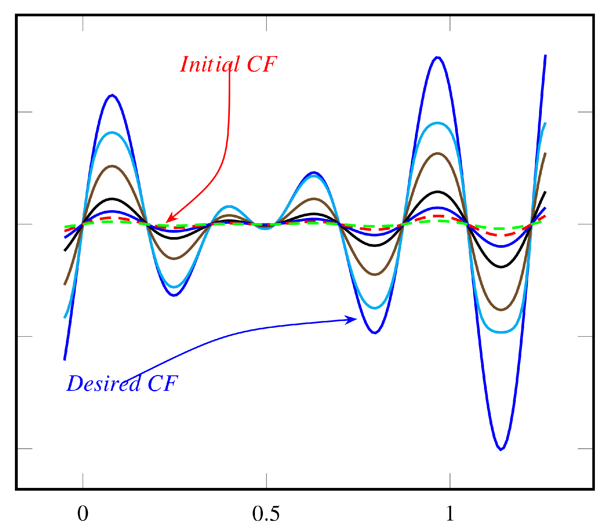
Although the present article uses simple structures for constructing functional homotopies, similar to those used in the well-known quantum annealing algorithm (linear combination of terminal functions), it is possible, and sometimes necessary, to employ nonlinear operations to attain the desired effects. In order to illustrate with examples, let us consider the functions and , and respective homotopies, displayed in Figure 2 and Figure 3. Of course, only a small number of intermediate functions are shown between the terminal functions, represented by the cited multimodal cost functions and almost constant functions. The homotopy itself is constructed by composing the function and the linear function .
It is also worth noticing that the ordinal configuration of local minima and their location are maintained, resulting in an ordered homotopy.
In summary, the homotopies used in the above examples may be defined as follows.
Figure 2.
Nonlinear homotopy → Cost function .
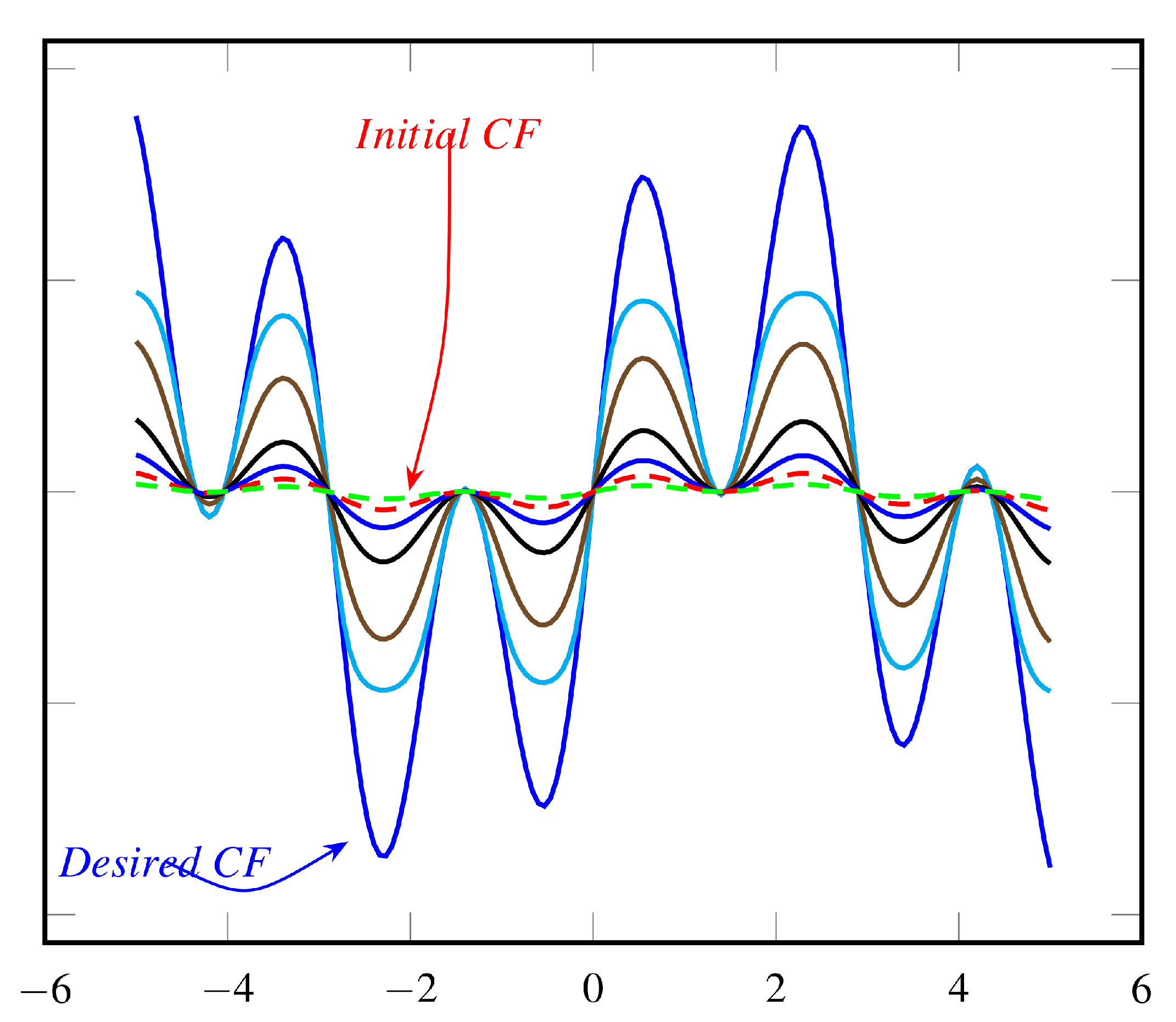
Figure 3.
Nonlinear homotopy → Cost function .
The proposed paradigm is to activate, in an independent way, the homotopic annealing process coupled to the usual mechansms of Fuzzy ASA, that may be faced as the well-known thermal annealing.This type of operation showed itself feasible by working outside the dynamics of ASA, actuating before each objective function evaluation and using the number of function evaluations as the annealing parameter. By doing so, the cost function continually changes its shape so as to facilitate the global landscape discovery activity. In terms of implementation, the corresponding code may be inserted into the module responsible for the calculation of the objective function. A description of a practical proposal follows:
- Define parameters corresponding to homotopic annealing (annealing strategy function, offset corresponding to initial function, sampling period etc.)
- In the module corresponding to cost function calculation, insert code to (after computing the actual value of the objective function) control the dynamics of HA process, that is (in C-like pseudocode):
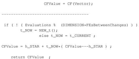
- Integrate the modified module with Fuzzy ASA and run the resulting program, as usual.
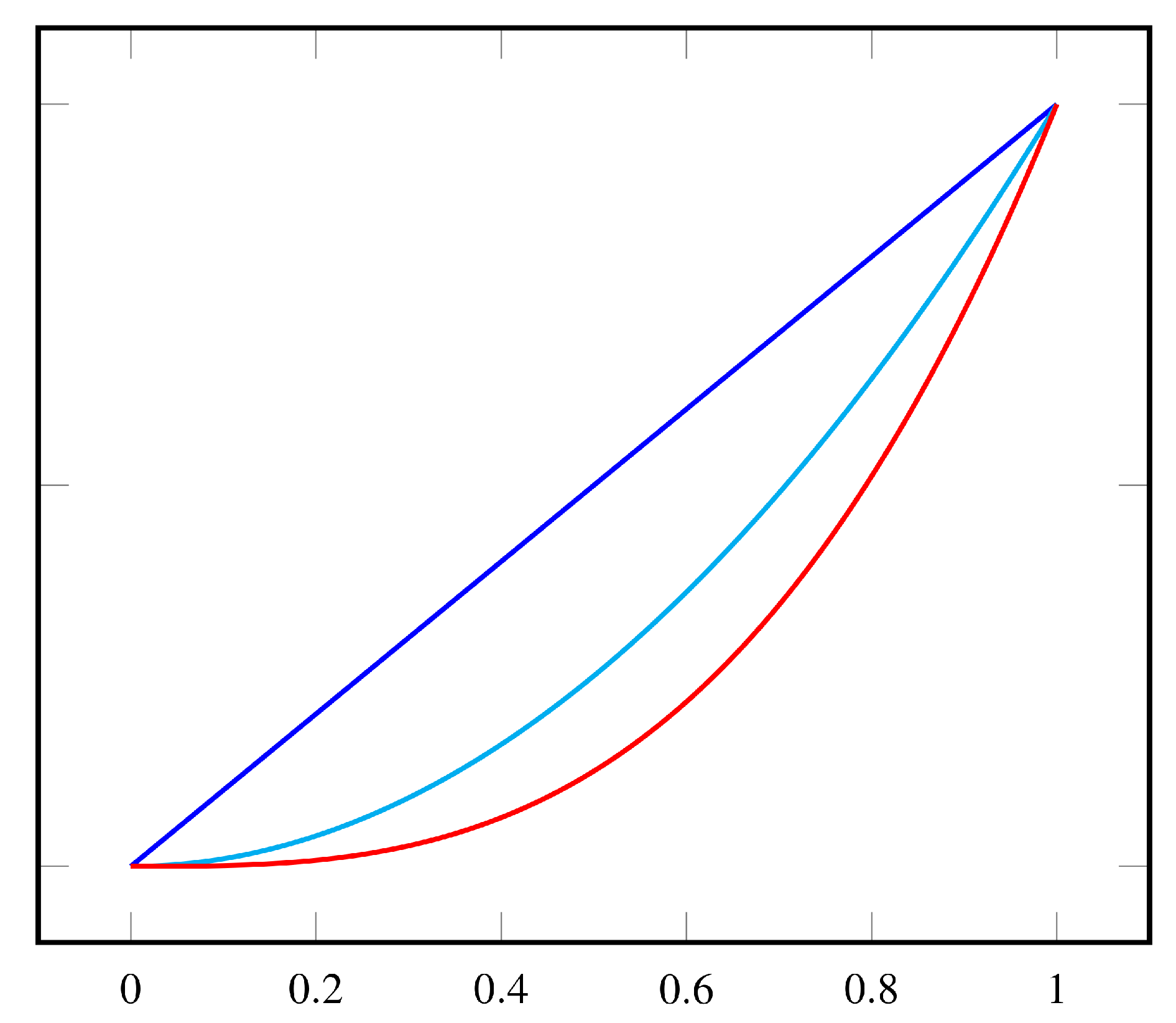
It is important to highlight that the homotopic annealing dynamical behavior can be customized so that the speed of the cost function variation may be tuned to each particular problem. For example, by using a linear function, the annealing rate is uniform. On the other hand, by using a quadratic function
(), the change rate is small in the beginning and becomes more intense during the final phase of the optimization session.
Figure 4.
Some possible homotopic annealing schedules.
In Figure 5 it is shown a generic fluxogram to illustrate the suggested procedure.
6. Numerical Results and Discussion
In this section several examples are presented along with respectives convergence graphs, pictures displaying instances of quantum tunneling and comparisons between results with and without activation of homotopic annealing.
The first function features a 2-dimensional domain, two deep local minima and only one global minimum, and was constructed to make it easier to obtain evidences about tunneling and related issues.
The second example uses a function with 2-dimensional domain, three local minima and was obtained by means of the excellent library GKLS, described in [10]. The GKLS apparatus allows users to synthesize three kinds of functions (non-differentiable, continuously differentiable and twice continuously differentiable) with known local and global minima, for testing multidimensional global optimization methods.
The third example concentrates mainly on the comparison of the optimzation performance with and without the activation of homotopic annealing. The well-known Rastrigin function is used, with a 20-dimensional domain.
6.1. Example—Smooth Bimodal Function with 2-dimensional Domain
Here the cost function is defined by
Domain
Its graph is displayed in Figure 6, Figure 7 and Figure 8, along with vertical indicators which will be used in this section.
In the figures, vertical lines indicate some points in the graphs where tunneling occurred: for example, starting from the point corresponding to the red line, and without the occurence of big uphill movements, it was possible to reach the basin of the global minimum, indicated by the blue line, with sampling taking place in another region of the domain. The same phenomenon occured to the pair indicated by lines with colors green and magenta—starting from the bottom of a local minimum (green line), and without "climbing" its attraction basin, it was possible to reach the desired global minimum attraction region (magenta line).
Minima:
GLOBAL with value
LOCAL with value
Below, the evolution of several minimization sessions is shown, with and without the activation of homotopic annealing.
Figure 9.
Minimization evolution without homotopic annealing.
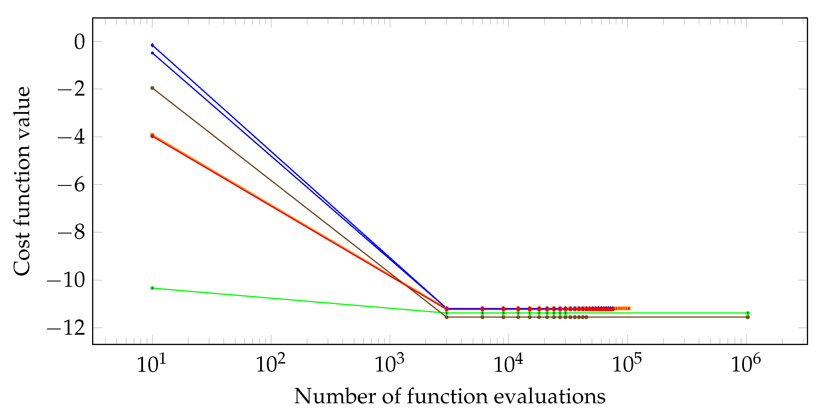
Figure 10.
Minimization evolution with homotopic annealing.
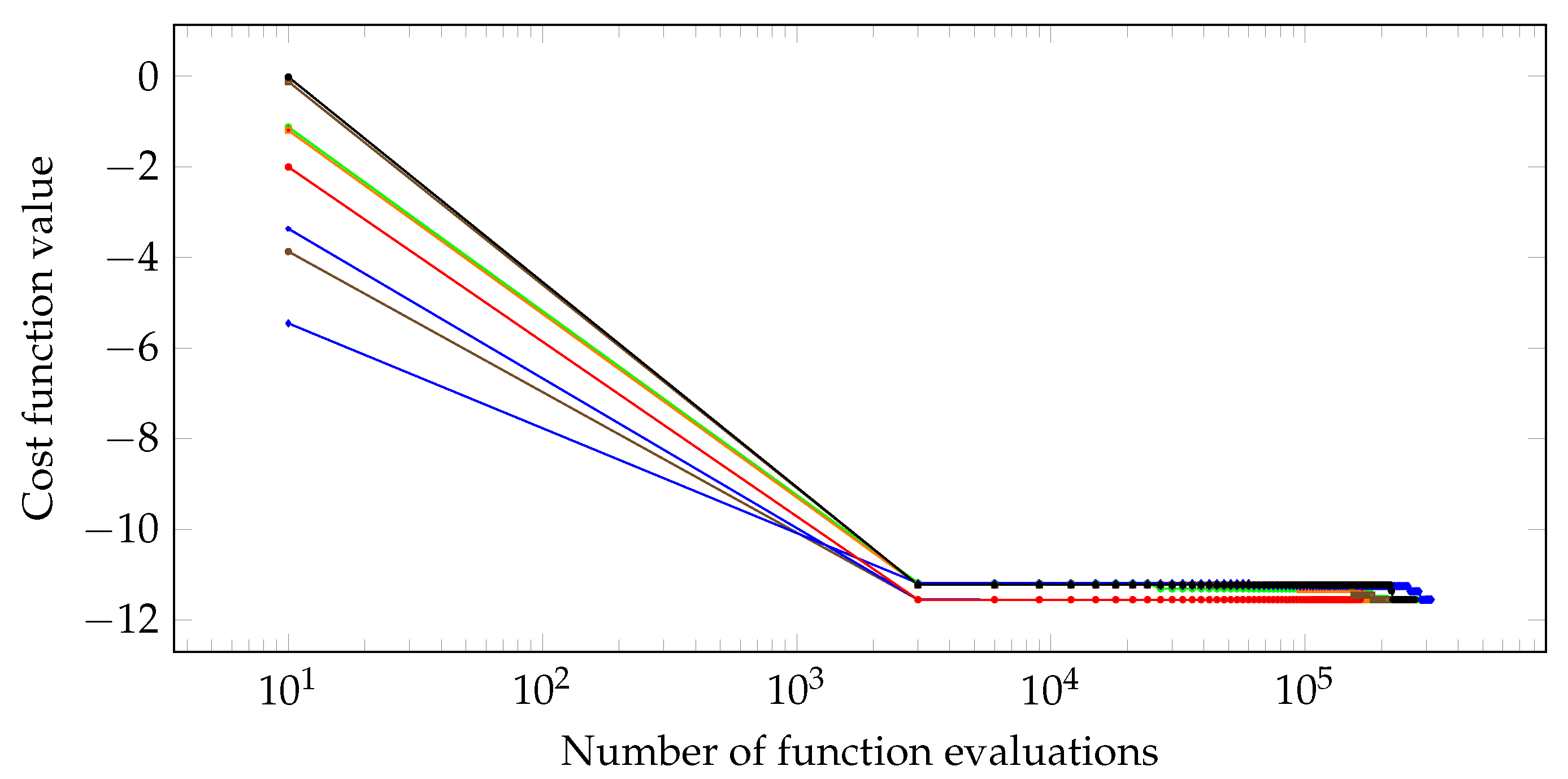
It is noticeable that all runs using homotopic annealing could reach the global minimum, while without its activation sometimes that does not happen. In addition, the occurence of quantum-like tunneling is very promising, given the inherent difficulty with convergence to suboptimal regions.
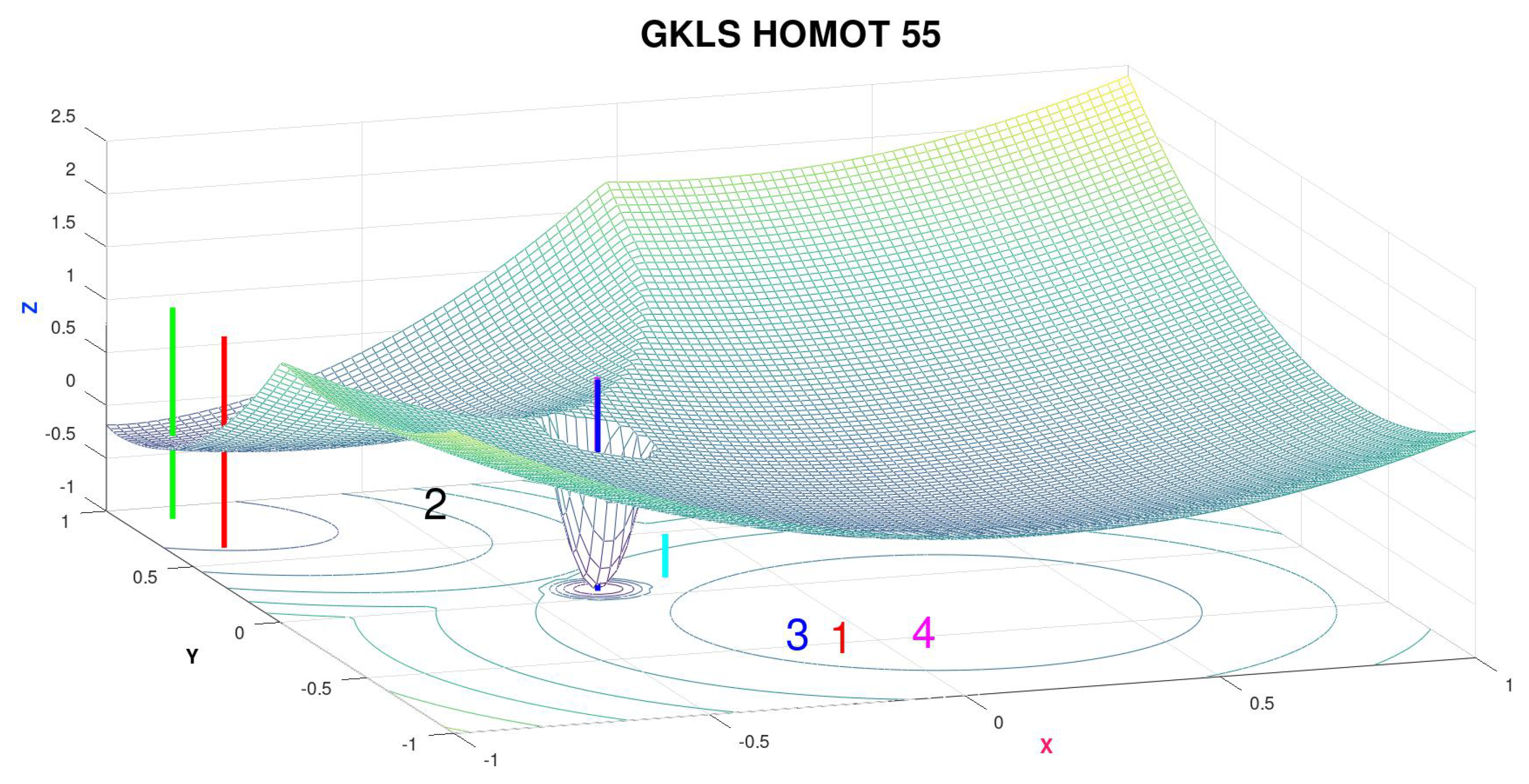
6.2. Example—Continuous Multimodal Function with 2-Dimensional Domain
Here the cost function is defined by test function number 55 within the class GKLS_ND_func described in [10].
Domain
Views of its graph are displayed in Figure 11 and Figure 12 along with some indicators which will be useful when describing the quantum-like characteristics of the superposition of homotopic and simulated annealing.
Global minimum value = −1 at (−0.3519657930556272, 0.08061776117282048)
Below, the evolution of several minimization sessions is shown, with and without the activation of homotopic annealing.
Figure 13.
Minimization evolution without homotopic annealing.
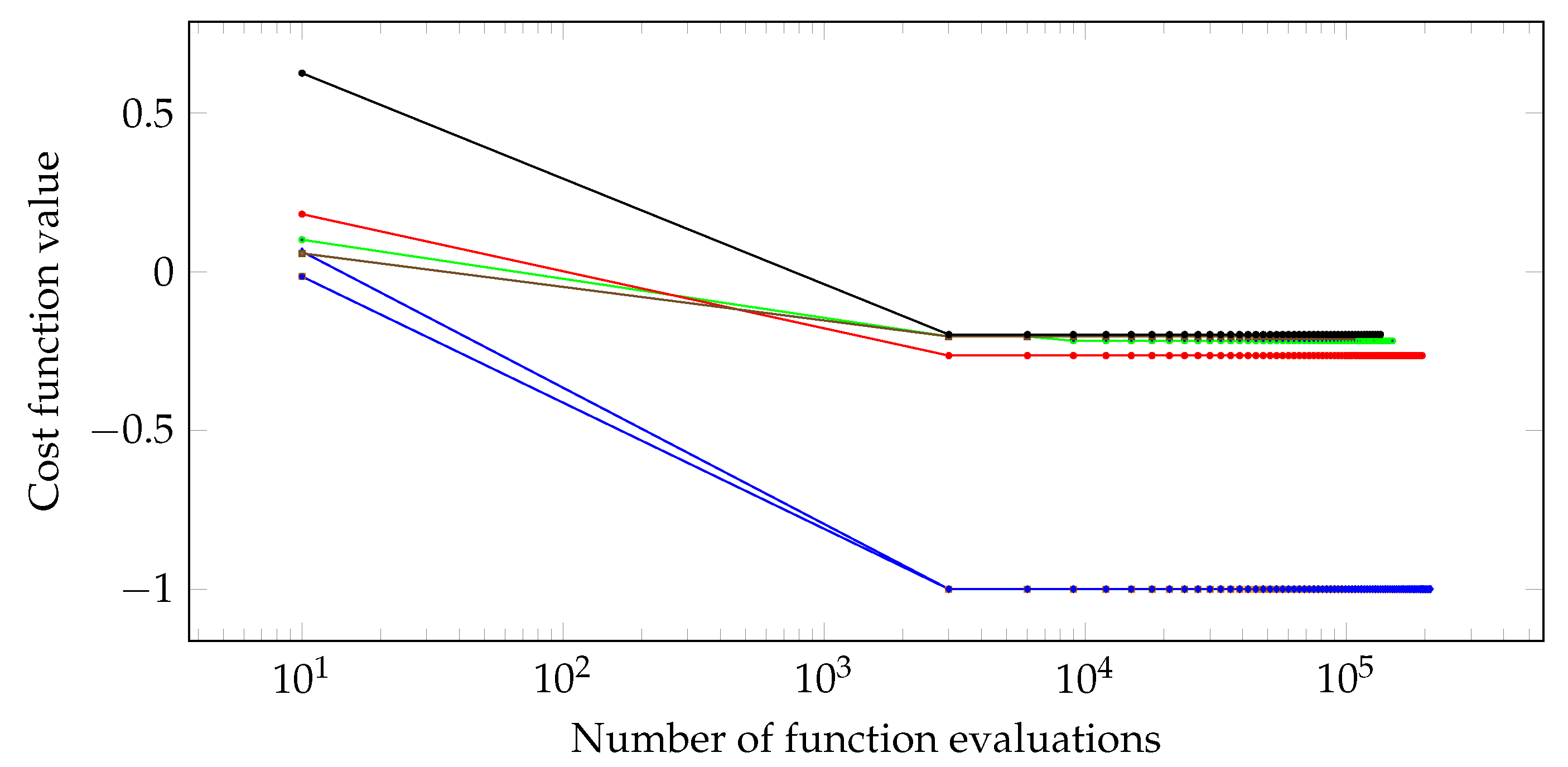
Figure 14.
Minimization evolution with homotopic annealing.
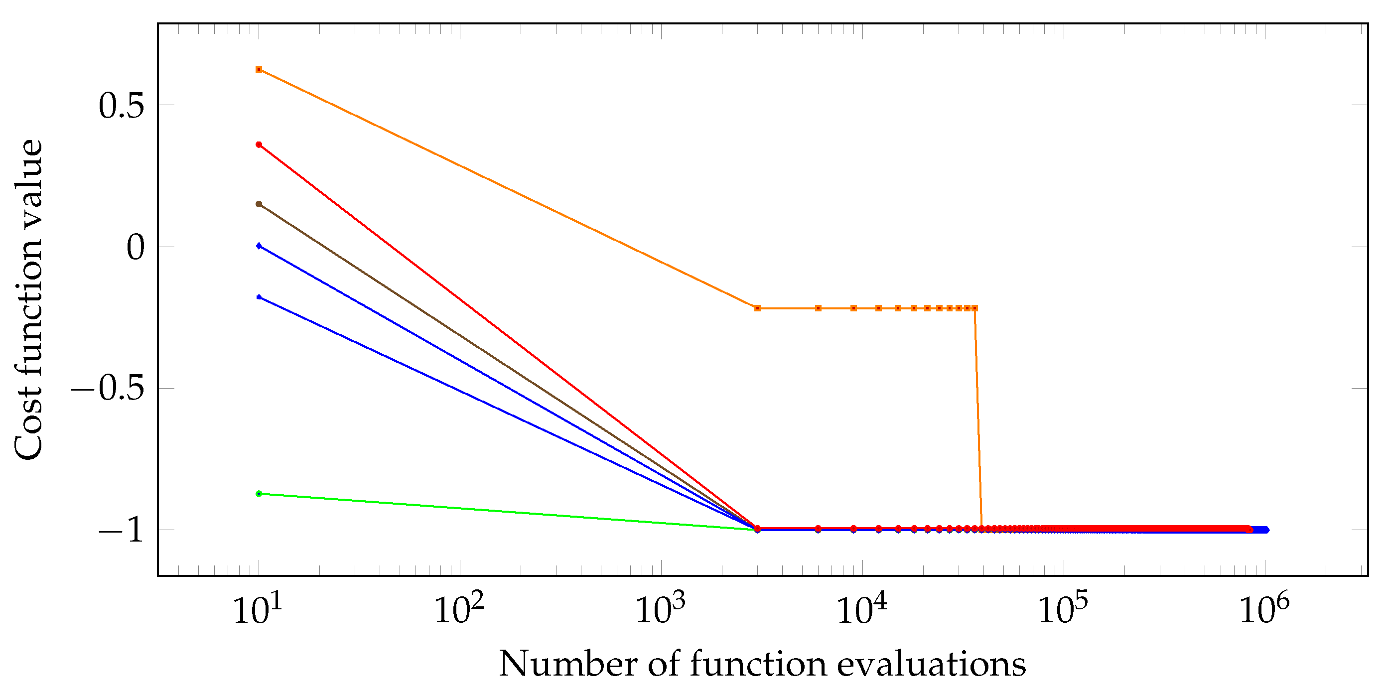
Here again it is possible to observe that, without the activation of homotopic annealing, some sessions did not converge to the global optimum. This kind of behavior is expected with "pure" thermal annealing, taking into account that initial points were located in suboptimal basins on purpose, as indicated by the red and green vertical bars, and the cyan sign. Furthermore, the numbers (1,2,3,4) represent the locations of the last samples produced immediately before the algorithm (with HA) enters the global minimum attraction basin, in a specific but typical optimization session—this dynamics evidences that sampling was taking place in distant regions and no uphill movement occurred induced by this type of process, indicating the existence of tunneling.
6.3. Example—Rastrigin Multimodal Function with 50-Dimensional Domain
The function is defined by (d=50)
Domain
Global minimum value is 0 at the origin of .
Below, the evolution of several minimization sessions is shown, with and without the activation of homotopic annealing.
Figure 15.
Minimization evolution without homotopic annealing.
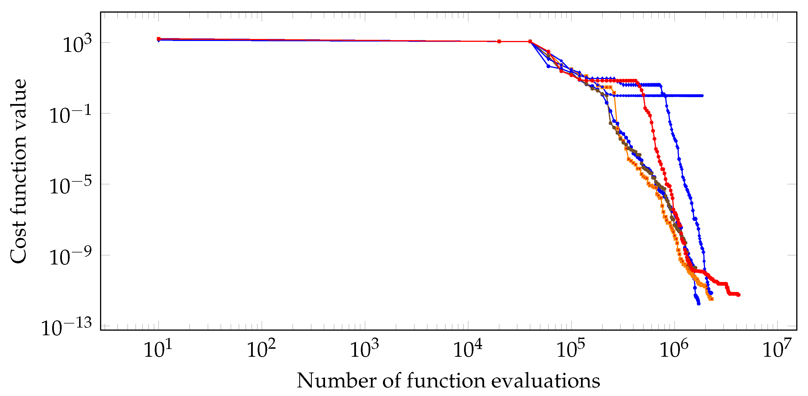
Figure 16.
Minimization evolution with homotopic annealing.
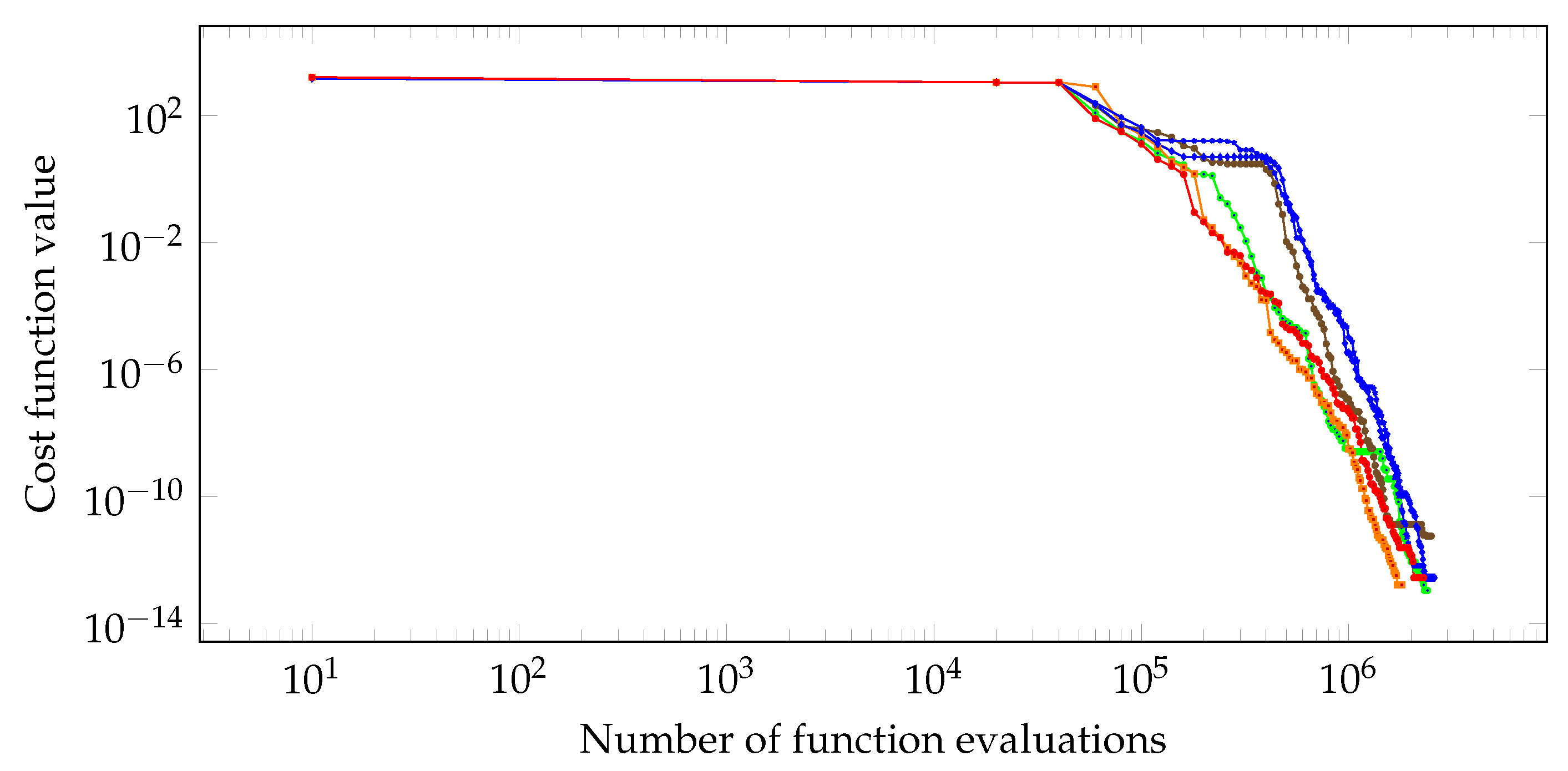
In this example the apparatus without homotopic annealing fails to converge to the global minimum in some runs, while all simulations with activation of HA are succesful, finding a very precise approximation for the true minimizer. Besides, in the former setting the obtained approximations reach values with order of , while in the latter this order goes to , that is, a reasonable improvement that can be attributed to the joint use of HA.
7. Conclusions
This paper proposed a global optimization framework which simultaneously combines two apparently independent types of annealing, provoking favorable phenomena like quantum tunneling through attraction basins, entanglement-like behavior between the two annealing dynamics and improvement in the overall efficacy, in terms of finding global optima. In order to demonstrate the reach and benefits of the presented approach, several results of representative examples are included, along with performance figures and illustrations for each case. Numerical tests confirm the quality of the approach, considering the contrast with and without the activation of the proposed algorithmic devices. One interesting and welcome aspect is that the observed computational overhead is minimal, despite the quantum-like obtained effects (and contrary to the general belief that such results would spend huge amounts of resources when simulated in present-day digital computers). Furthermore, it was suggested that, taking into account the availability of commercial quantum annealers [1], it would be interesting to implement the ideas conveyed in the proposed approach in such devices.
References
- S. A. Abel, L. A. Nutricati, Ising Machines for Diophantine Problems in Physics, Progress in Physics, Volume 70, Issue 11, 2022. [CrossRef]
- B. Apolloni, C. Carvalho, D. de Falco, Quantum stochastic optimization. Stoc. Proc. Appl. 33 2 pp. 223-244, 1989. [CrossRef]
- Apolloni, N. Cesa-Bianchi, D. de Falco, A numerical implementation of Quantum Annealing, in Stochastic Processes, Physics and Geometry, Proceedings of the Ascona/Locarno Conference, Albeverio et al. Eds., World Scientific, 97-111, 1990.
- B. Just, Quantum Computing Compact—Spooky Action at a Distance and Teleportation Easy to Understand, Springer-Verlag, Berlin, 2022. [CrossRef]
- V. Bapst, G. Semerjian, Thermal, quantum and simulated quantum annealing: analytical comparisons for simple models, J. Phys.: Conf. Ser. 473 012011, 2013. [CrossRef]
- D. A. Battaglia, L. Stella, Optimization through quantum annealing: theory and some applications, Contemporary Physics, 47:4, 195-208, 2006. [CrossRef]
- F. J. Duarte, Fundamentals of Quantum Entanglement, IOP Publishing, London, 2019.
- A. Einstein, B. Podolsky, N. Rosen. Can quantum-mechanical description of physical reality be considered complete? Phys. Rev. 47 777-780, 1935. [CrossRef]
- D. de Falco, D. Tamascelli, AN INTRODUCTION TO QUANTUM ANNEALING, RAIRO-Theor. Inf. Appl. 45 99-116, 2011. [CrossRef]
- Gaviano, M., Lera, D., Kvasov, D.E., Sergeyev, Y.D.: Algorithm 829 Software for generation of classes of test functions with known local and global minima for global optimization. ACM Trans. Math. Software 29, 469-480 (2003). [CrossRef]
- L. Ingber. Adaptive simulated annealing (ASA): Lessons learned. Control and Cybernetics 25 (1) 33-54, 1996. [CrossRef]
- C. C. McGeoch, Adiabatic Quantum Computation and Quantum Annealing: Theory and Practice, Morgan & Claypool, 2014. [CrossRef]
- H. A. Oliveira Jr., L. Ingber, A. Petraglia, M.R. Petraglia, M.A.S. Machado, Stochastic Global Optimization and Its Applications with Fuzzy Adaptive Simulated Annealing, Springer-Verlag, Berlin-Heidelberg, 2012. [CrossRef]
- H. A. Oliveira Jr., Evolutionary Global Optimization, Manifolds and Applications, Springer-Verlag, Cham Heidelberg New York Dordrecht London, 2016. [CrossRef]
- H.A. Oliveira Jr., A. Petraglia, Global optimization using space-filling curves and measure-preserving transformations, in: A. Gaspar-Cunha et al. (Eds.), Soft Computing in Industrial Applications, AISC 96, Springer-Verlag, Berlin Heidelberg, 2011, pp. 121-130. [CrossRef]
- S. Kirkpatrick, C. D. Gelatt Jr., M. P. Vecchi, Science 220, 671, 1983.
- D. Tamaki, FIBER BUNDLES AND HOMOTOPY, World Scientific, 2021. [CrossRef]
Figure 1.
Simulated annealing basin hopping and quantum tunneling.
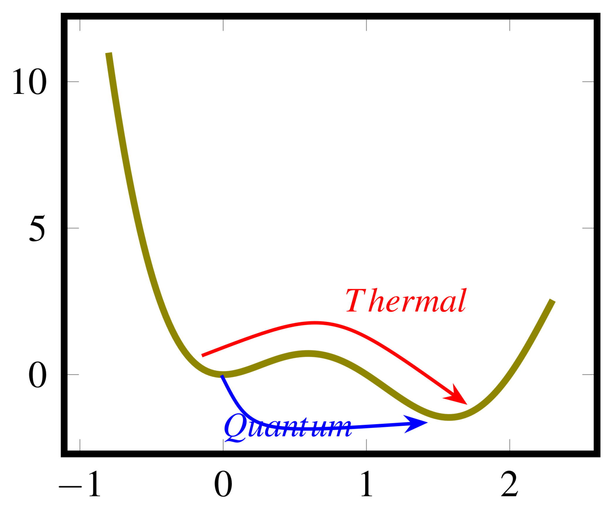
Figure 5.
Overview of the proposed algorithm.
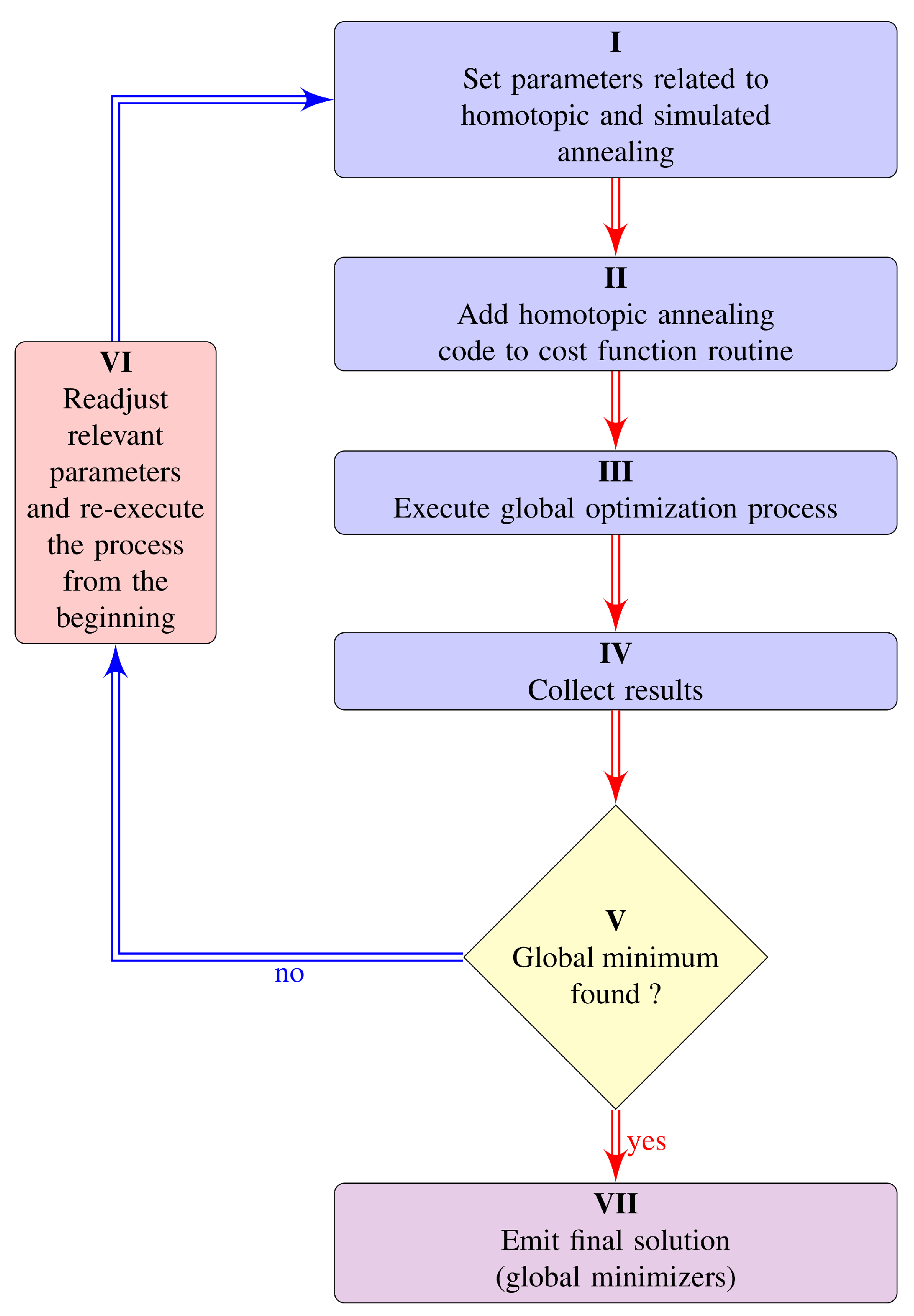
Figure 6.
Cost function for example.
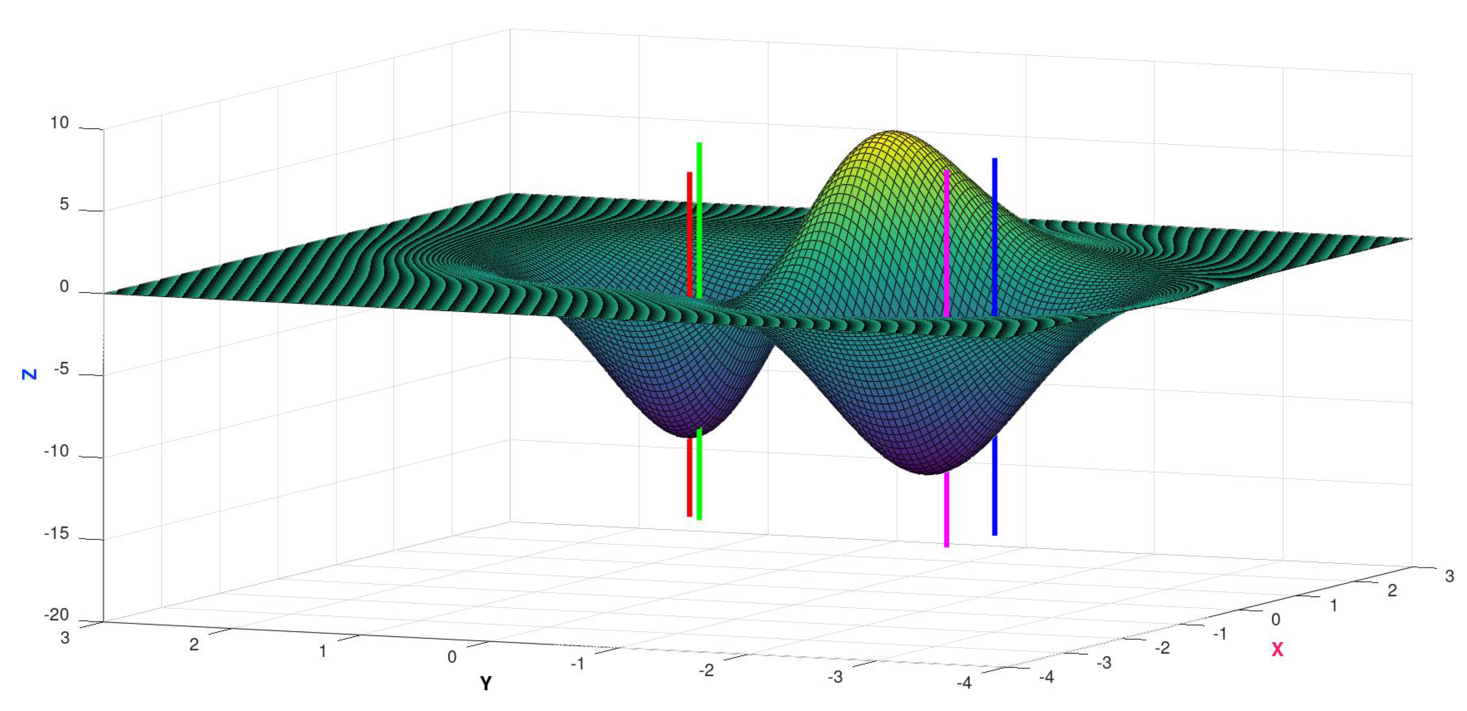
Figure 7.
Another view.
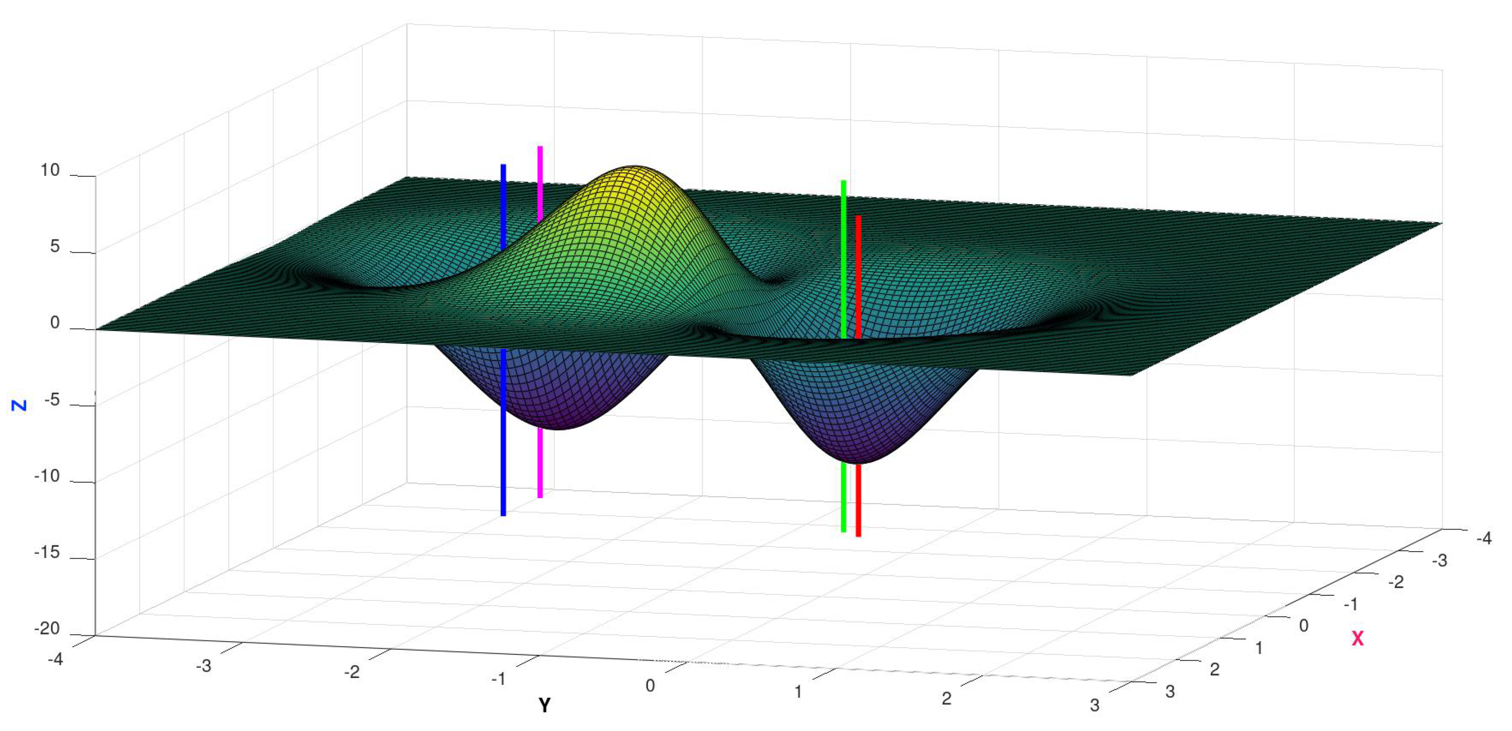
Figure 8.
Another view.
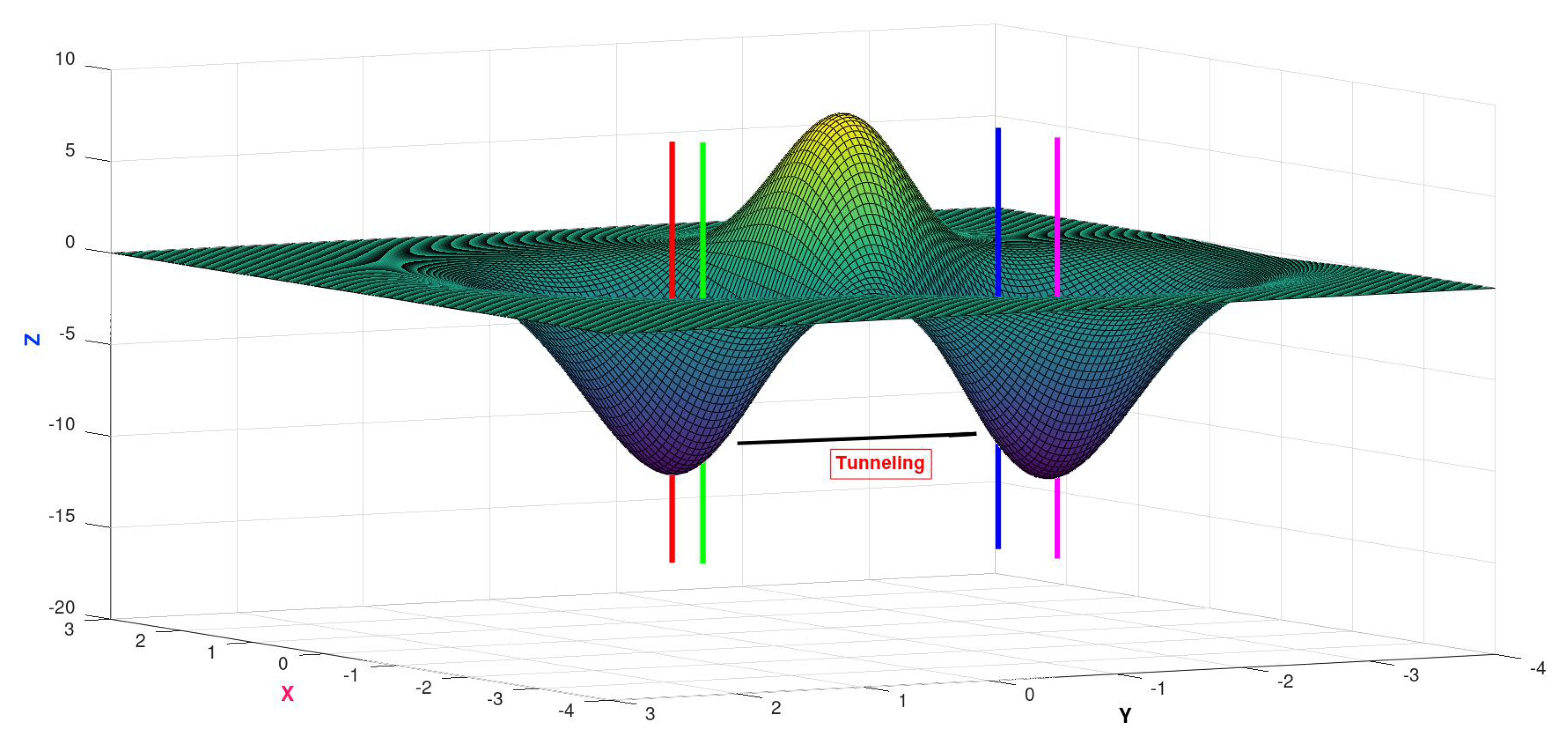
Figure 11.
Cost function for example.
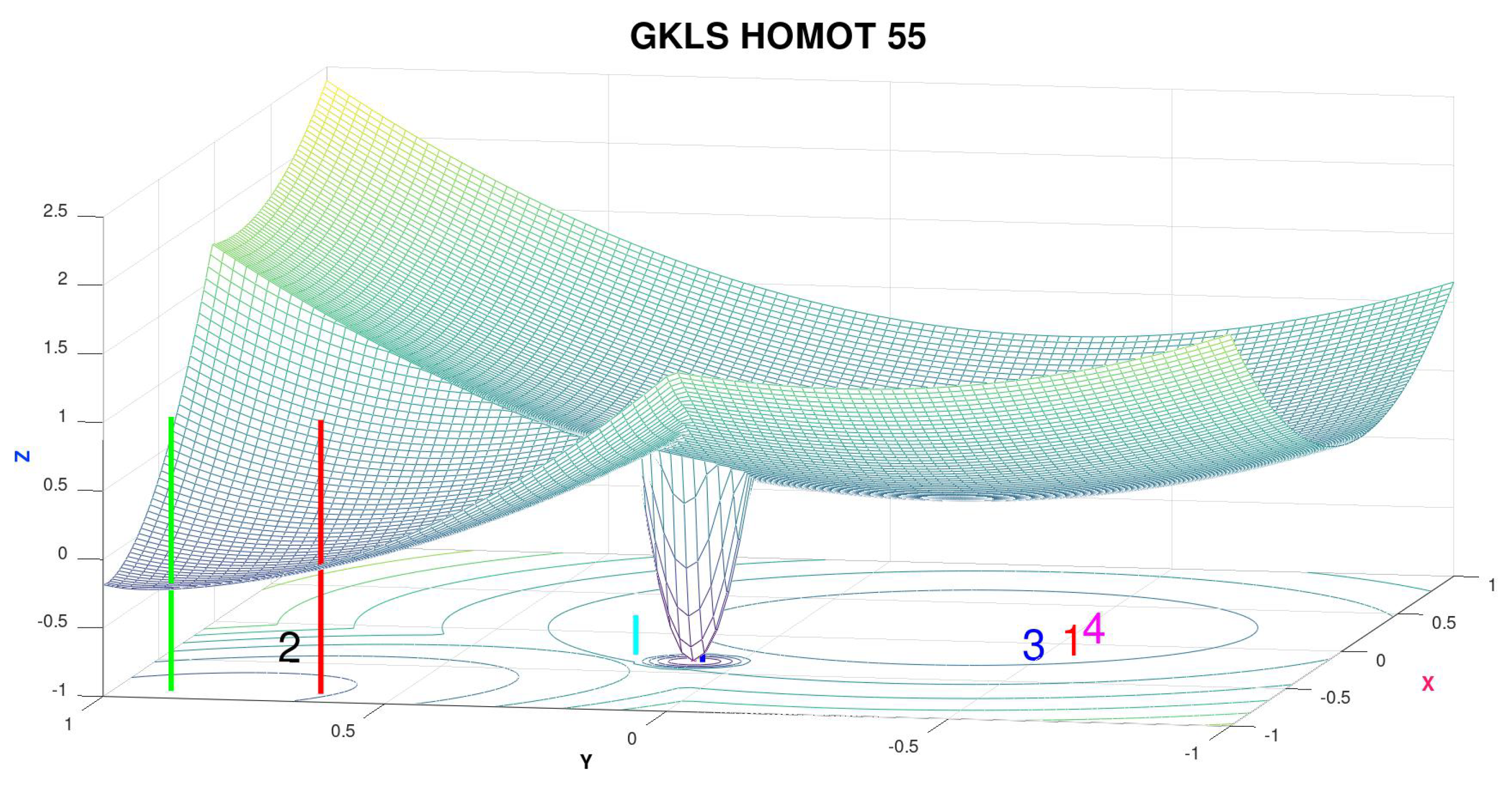
Figure 12.
Another view.
Disclaimer/Publisher’s Note: The statements, opinions and data contained in all publications are solely those of the individual author(s) and contributor(s) and not of MDPI and/or the editor(s). MDPI and/or the editor(s) disclaim responsibility for any injury to people or property resulting from any ideas, methods, instructions or products referred to in the content. |
© 2023 by the authors. Licensee MDPI, Basel, Switzerland. This article is an open access article distributed under the terms and conditions of the Creative Commons Attribution (CC BY) license (http://creativecommons.org/licenses/by/4.0/).
Copyright: This open access article is published under a Creative Commons CC BY 4.0 license, which permit the free download, distribution, and reuse, provided that the author and preprint are cited in any reuse.


