

Submitted:
27 March 2023
Posted:
27 March 2023
Read the latest preprint version here
Abstract
This article develops duality principles and numerical results for a large class of non-convex variational models. The main results are based on fundamental tools of convex analysis, duality theory and calculus of variations. More specifically the approach is established for a class of non-convex functionals similar as those found in some models in phase transition. Finally, in the last section we present a concerning numerical example and the respective software.
Keywords:
Duality theory
; non-convex analysis
; numerical method for a non-smooth model
MSC: 49N15
1. Introduction
In this section we establish a dual formulation for a large class of models in non-convex optimization.
The main duality principle is applied to double well models similar as those found in the phase transition theory.
Such results are based on the works of J.J. Telega and W.R. Bielski [2,3,14,15] and on a D.C. optimization approach developed in Toland [16].
About the other references, details on the Sobolev spaces involved are found in [1]. Related results on convex analysis and duality theory are addressed in [5,6,7,9,13].
Finally, in this text we adopt the standard Einstein convention of summing up repeated indices, unless otherwise indicated.
In order to clarify the notation, here we introduce the definition of topological dual space.
Definition 1.1
(Topological dual spaces). Let U be a Banach space. We shall define its dual topological space, as the set of all linear continuous functionals defined on U. We suppose such a dual space of U, may be represented by another Banach space , through a bilinear form (here we are referring to standard representations of dual spaces of Sobolev and Lebesgue spaces). Thus, given linear and continuous, we assume the existence of a unique such that
The norm of f , denoted by , is defined as
At this point we start to describe the primal and dual variational formulations.
2. A General Duality Principle Non-Convex Optimization
In this section we present a duality principle applicable to a model in phase transition.
This case corresponds to the vectorial one in the calculus of variations.
Let be an open, bounded, connected set with a regular (Lipschitzian) boundary denoted by
Consider a functional where
and where
and
We assume there exists such that
Moreover, suppose F and G are Fréchet differentiable but not necessarily convex. A global optimum point may not be attained for J so that the problem of finding a global minimum for J may not be a solution.
Anyway, one question remains, how the minimizing sequences behave close the infimum of J.
We intend to use duality theory to approximately solve such a global optimization problem.
Denoting , , , at this point we define, , , , and by
and
and
Define now ,
Observe that
.
Here we assume are large enough so that and are convex.
Hence, from the general results in [16], we may infer that
On the other hand
where refers to a standard quasi-convex regularization of J.
From these last two results we may obtain
Moreover, from standards results on convex analysis, we may have
where
and
Thus, defining
we have got
Finally, observe that
This last variational formulation corresponds to a concave relaxed formulation in concerning the original primal formulation.
3. Another Duality Principle for a Simpler Related Model in Phase Transition with a Respective Numerical Example
In this section we present another duality principle for a related model in phase transition.
Let and consider a functional where
and where
and
A global optimum point is not attained for J so that the problem of finding a global minimum for J has no solution.
Anyway, one question remains, how the minimizing sequences behave close the infimum of J.
We intend to use duality theory to approximately solve such a global optimization problem.
Denoting , at this point we define, and by
and
Observe
where refers to a quasi-convex regularization of
We define also
and
by
and
Observe that if is large enough, both and G are convex.
Denoting we also define the polar functional by
Observe that
With such results in mind, we define a relaxed primal dual variational formulation for the primal problem, represented by , where
Having defined such a functional, we may obtain numerical results by solving a sequence of convex auxiliary sub-problems, through the following algorithm.
- Set and and
- Choose such that and
- Set
- Calculate solution of the system of equations:andthat isandso thatand
- Calculate by solving the system of equations:andthat isand
- If , then stop, else set and go to item 4.
For the case in which , we have obtained numerical results for and . For such a concerning solution obtained, please see Figure 1. For the case in which , we have obtained numerical results for and . For such a concerning solution obtained, please see Figure 2.
Remark 3.1.
Observe that the solutions obtained are approximate critical points. They are not, in a classical sense, the global solutions for the related optimization problems. Indeed, such solutions reflect the average behavior of weak cluster points for concerning minimizing sequences.
4. A Convex Dual Variational Formulation for a Third Similar Model
In this section we present another duality principle for a third related model in phase transition.
Let and consider a functional where
and where
and
A global optimum point is not attained for J so that the problem of finding a global minimum for J has no solution.
Anyway, one question remains, how the minimizing sequences behave close to the infimum of J.
We intend to use the duality theory to solve such a global optimization problem in an appropriate sense to be specified.
At this point we define, and by
and
Denoting we also define the polar functional and by
and
Observe this is the scalar case of the calculus of variations, so that from the standard results on convex analysis, we have
Indeed, from the direct method of the calculus of variations, the maximum for the dual formulation is attained at some .
Moreover, the corresponding solution is obtained from the equation
Finally, the Euler-Lagrange equations for the dual problem stands for
where if if and
if
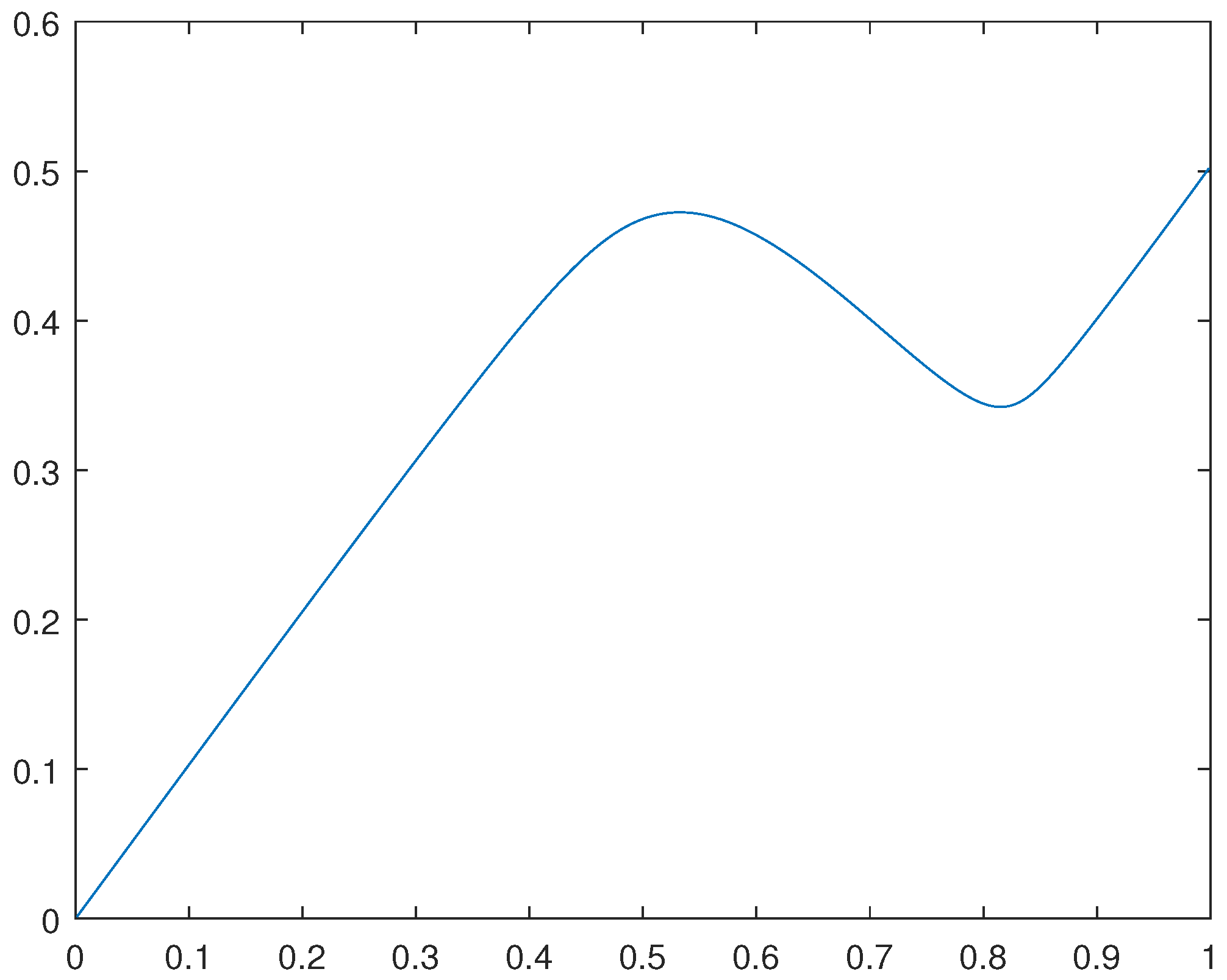
We have computed the solutions and corresponding solutions for the cases in which and
For the solution for the case in which , please see Figure 3.
For the solution for the case in which , please see Figure 4.
Remark 4.1.
Observe that such solutions obtained are not the global solutions for the related primal optimization problems. Indeed, such solutions reflect the average behavior of weak cluster points for concerning minimizing sequences.
4.1. The Algorithm Through Which We Have Obtained the Numerical Results
In this subsection we present the software in MATLAB through which we have obtained the last numerical results.
This algorithm is for solving the concerning Euler-Lagrange equations for the dual problem, that is, for solving the equation
Here the concerning software in MATLAB. We emphasize to have used the smooth approximation
where a small value for is specified in the next lines.
*************************************
- clear all
- (number of nodes)
-
(we have fixed the number of iterations)
********************************
5. An Improvement of the Convexity Conditions for a Non-Convex Related Model Through an Approximate Primal Formulation
In this section we develop an approximate primal dual formulation suitable for a large class of variational models.
Here, the applications are for the Kirchhoff-Love plate model, which may be found in Ciarlet, [10].
At this point we start to describe the primal variational formulation.
Let be an open, bounded, connected set which represents the middle surface of a plate of thickness h. The boundary of , which is assumed to be regular (Lipschitzian), is denoted by . The vectorial basis related to the cartesian system is denoted by , where (in general Greek indices stand for 1 or 2), and where is the vector normal to , whereas and are orthogonal vectors parallel to Also, is the outward normal to the plate surface.
The displacements will be denoted by
The Kirchhoff-Love relations are
Here so that we have where
It is worth emphasizing that the boundary conditions here specified refer to a clamped plate.
We also define the operator , where , by
The constitutive relations are given by
where: and , are symmetric positive definite fourth order tensors. From now on, we denote and .
Furthermore denote the membrane force tensor and the moment one. The plate stored energy, represented by is expressed by
and the external work, represented by , is given by
where are external loads in the directions , and respectively. The potential energy, denoted by is expressed by:
Define now by
where
In such a case for , , in and
we get
and
This new functional has a relevant improvement in the convexity conditions concerning the previous functional J.
Indeed, we have obtained a gain in positiveness for the second variation which has increased of order
Moreover the difference between the approximate and exact equation
is of order which corresponds to a small perturbation in the original equation for a load of for example. Summarizing, the exact equation may be approximately solved in an appropriate sense.
6. An Approximate Convex Variational Formulation for Another Related Model
In this section, we obtain an approximate convex variational formulation for a related model, more specifically, for a Ginzburg-Landau type equation.
Let be an open, bounded and connected set with a regular (Lipschitzian) boundary denoted by
Consider a functional where
where , , , and
We define
and
At this point we define so that
Moreover we define
and where
where
Here , , , in and
and
Thus, with such numerical values, we may obtain
and
Remark 6.1.
This new functional has a relevant improvement in the convexity conditions concerning the previous functional J.
Indeed, we have obtained a gain in positiveness for the second variation which has increased of order
Moreover the difference between the approximate and exact equation
is of order which for appropriate parameters and , corresponds to a small perturbation in the original equation. Summarizing, the exact equation may be approximately solved in an appropriate sense.
Finally, for this last example, we highlight it is relatively easy to improve even more both such an approximation quality and the convexity conditions concerning the original variational model.
With such statements and results in mind, we may prove the following theorem.
Theorem 6.2.
Suppose and are such that
in
Assume also, is such that
Under such hypotheses, is convex on so that
Moreover,
where
Proof.
From the hypotheses
in , so that is convex on the convex set
Consequently, since , we obtain
Finally, from the approximation indicated in the last remark and we get
The proof is complete.
□
7. An Exact Convex Dual Variational Formulation for a Non-Convex Primal One
In this section we develop a convex dual variational formulation suitable to compute a critical point for the corresponding primal one.
Let be an open, bounded, connected set with a regular (Lipschitzian) boundary denoted by
Consider a functional where
and
Here we denote and
Defining
for some appropriate , suppose also F is twice Fréchet differentiable and
Define now and by
and
where here we denote
Moreover, we define the respective Legendre transform functionals and as
where are such that
and
where are such that
Here is any function such that
Furthermore, we define
Observe that through the target conditions
we may obtain the compatibility condition
Define now
for some appropriate such that is convex in
Consider the problem of minimizing subject to
Assuming is large enough so that the restriction in r is not active, at this point we define the associated Lagrangian
where is an appropriate Lagrange multiplier.
Therefore
The optimal point in question will be a solution of the corresponding Euler-Lagrange equations for
From the variation of in we obtain
From the variation of in we obtain
From the variation of in we have
From this last equation, we may obtain such that
and
From this and the previous extremal equations indicated we have
and
so that
and
Replacing the expressions of and into this last equation, we have
so that
Observe that if
then there exists such that u and are also such that
and
The boundary conditions for must be such that
From this and Equation (33) we obtain
Summarizing, we may obtain a solution of equation by minimizing on .
Finally, observe that clearly is convex in an appropriate large ball for some appropriate
8. Another Primal Dual Formulation for a Related Model
Let be an open, bounded and connected set with a regular boundary denoted by
Consider the functional where
, and
Denoting , define now by
Define also
and
for some appropriate to be specified.
Moreover define
for some appropriate to be specified.
Observe that, denoting
we have
and
so that
Observe now that a critical point and in .
Therefore, for an appropriate large , also at a critical point, we have
Remark 8.1.
From this last equation we may observe that has a large region of convexity about any critical point , that is, there exists a large such that is convex on
With such results in mind, we may easily prove the following theorem.
Theorem 8.2.
Assume and suppose is such that
Under such hypotheses, there exists such that is convex in ,
and
9. A Third Primal Dual Formulation for a Related Model
Let be an open, bounded and connected set with a regular boundary denoted by
Consider the functional where
, and
Denoting , define now by
Define also
and
for some appropriate to be specified.
Moreover define
and
for some appropriate real constants to be specified.
Observe that we may obtain
and
so that
With such results in mind, we may easily prove the following theorem.
Theorem 9.1.
Assume and and suppose is such that
and
Assume also
Under such hypotheses, we have that
and
Proof.
The proof that
and
may be easily made similarly as in the previous sections.
Moreover, from the hypotheses,
and
From this, a standard saddle point theorem and the remaining hypotheses, we may infer that
The proof is complete. □
10. A Fourth Primal Dual Formulation for a Related Model
Let be an open, bounded and connected set with a regular boundary denoted by
Consider the functional where
, and
Denoting , define now by
where is a small real constant.
Define also
and
for some appropriate to be specified.
Moreover define
and
for some appropriate real constants to be specified.
Observe that, defining
we may obtain
and
so that
However, at a critical point, we have so that, we define
From such results, assuming define now
With such results in mind, we may easily prove the following theorem.
Theorem 10.1.
Suppose is such that
Under such hypotheses, we have that
and
Proof.
The proof that
and
may be easily made similarly as in the previous sections.
Moreover, from the hypotheses, we have
and
From this, from a standard saddle point theorem and the remaining hypotheses, we may infer that
Moreover, observe that
Summarizing, we have got
From such results, we may infer that
The proof is complete. □
References
- R.A. Adams and J.F. Fournier, Sobolev Spaces, 2nd edn. (Elsevier, New York, 2003).
- W.R. Bielski, A. Galka, J.J. Telega, The Complementary Energy Principle and Duality for Geometrically Nonlinear Elastic Shells. I. Simple case of moderate rotations around a tangent to the middle surface. Bulletin of the Polish Academy of Sciences, Technical Sciences, Vol. 38, No. 7-9, 1988.
- W.R. Bielski and J.J. Telega, A Contribution to Contact Problems for a Class of Solids and Structures, Arch. Mech., 37, 4-5, pp. 303-320, Warszawa 1985.
- J.F. Annet, Superconductivity, Superfluids and Condensates, 2nd edn. ( Oxford Master Series in Condensed Matter Physics, Oxford University Press, Reprint, 2010). 2010.
- F.S. Botelho, Functional Analysis, Calculus of Variations and Numerical Methods in Physics and Engineering, CRC Taylor and Francis, Florida, 2020.
- F.S. Botelho, Variational Convex Analysis, Ph.D. thesis, Virginia Tech, Blacksburg, VA -USA, (2009).
- F. Botelho, Topics on Functional Analysis, Calculus of Variations and Duality, Academic Publications, Sofia, (2011).
- F. Botelho, Existence of solution for the Ginzburg-Landau system, a related optimal control problem and its computation by the generalized method of lines. Applied Mathematics and Computation 2012, 218, 11976–11989. [CrossRef]
- F. Botelho, Functional Analysis and Applied Optimization in Banach Spaces, Springer Switzerland, 2014.
- P.Ciarlet, Mathematical Elasticity, Vol. II – Theory of Plates, North Holland Elsevier (1997).
- J.C. Strikwerda, Finite Difference Schemes and Partial Differential Equations, SIAM, second edition (Philadelphia, 2004).
- L.D. Landau and E.M. Lifschits, Course of Theoretical Physics, Vol. 5- Statistical Physics, part 1. (Butterworth-Heinemann, Elsevier, reprint 2008).
- R.T. Rockafellar, Convex Analysis, Princeton Univ. Press, (1970).
- J.J. Telega, On the complementary energy principle in non-linear elasticity. Part I: Von Karman plates and three dimensional solids, C.R. Acad. Sci. Paris, Serie II, 308, 1193-1198; Part II: Linear elastic solid and non-convex boundary condition. Minimax approach, ibid, pp. 1313-1317 (1989).
- A.Galka and J.J.Telega Duality and the complementary energy principle for a class of geometrically non-linear structures. Part I. Five parameter shell model; Part II. Anomalous dual variational priciples for compressed elastic beams. Arch. Mech. 1995, 47, 677-698, 699-724.
- J.F. Toland, A duality principle for non-convex optimisation and the calculus of variations. Arch. Rat. Mech. Anal. 1979, 71, 41–61. [CrossRef]
Figure 1.
solution for the case .
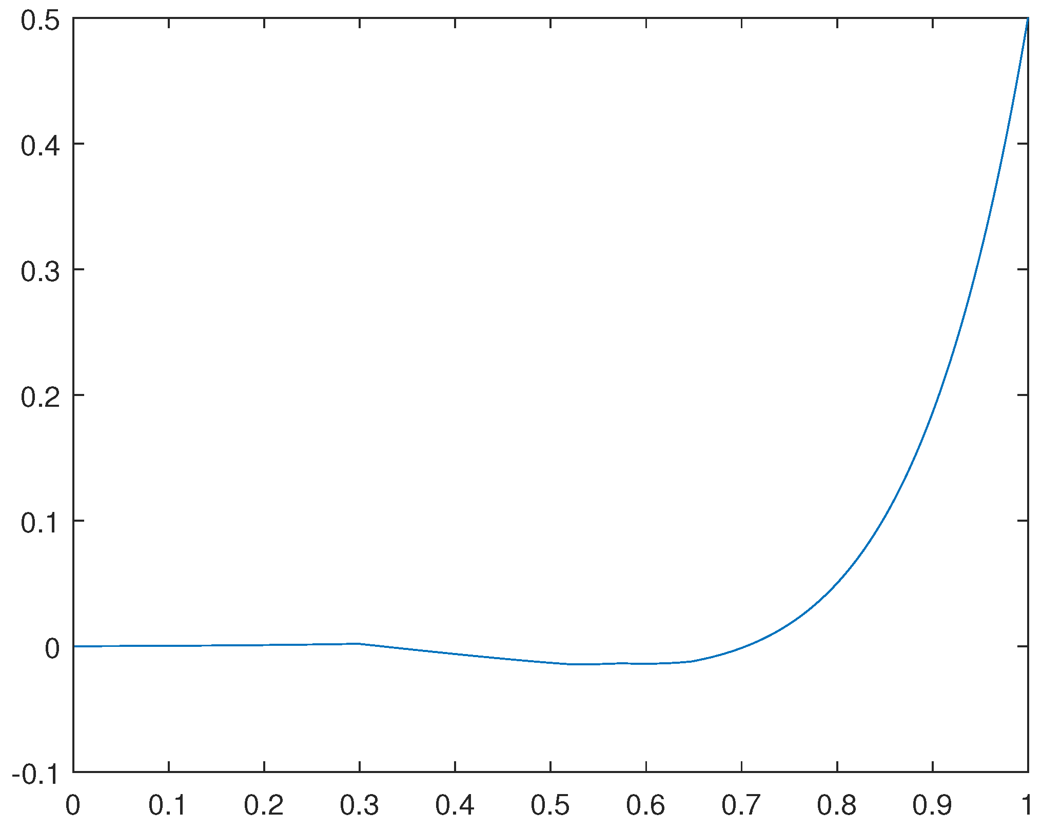
Figure 2.
solution for the case .
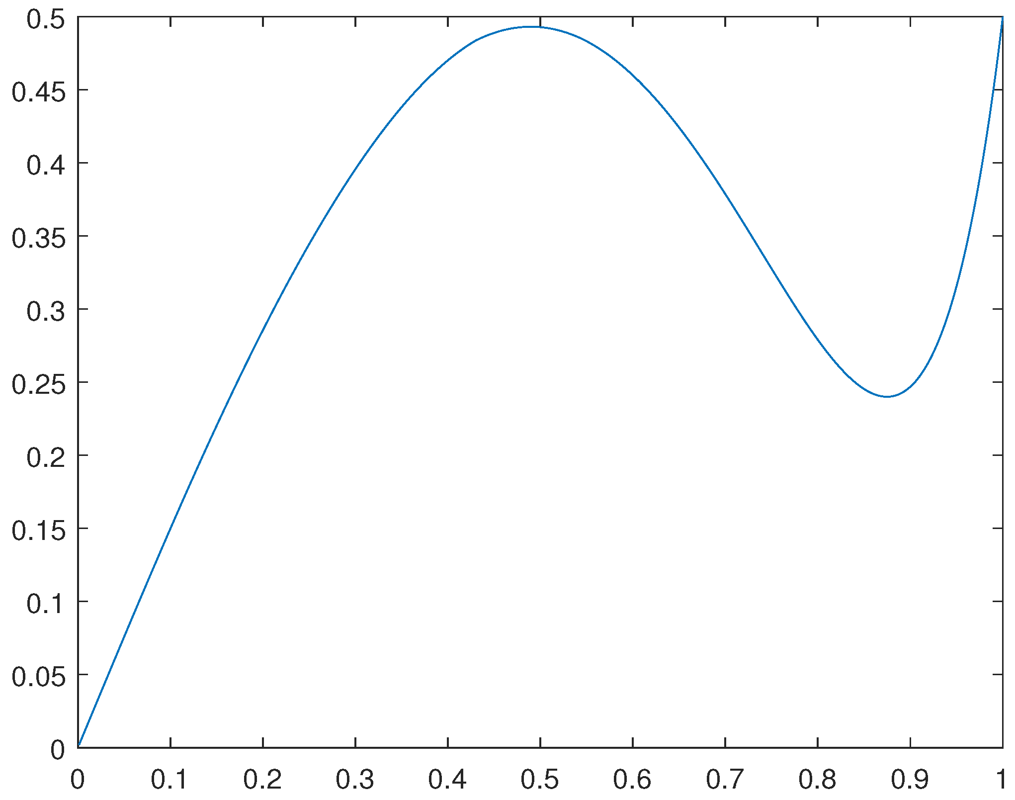
Figure 3.
solution for the case .
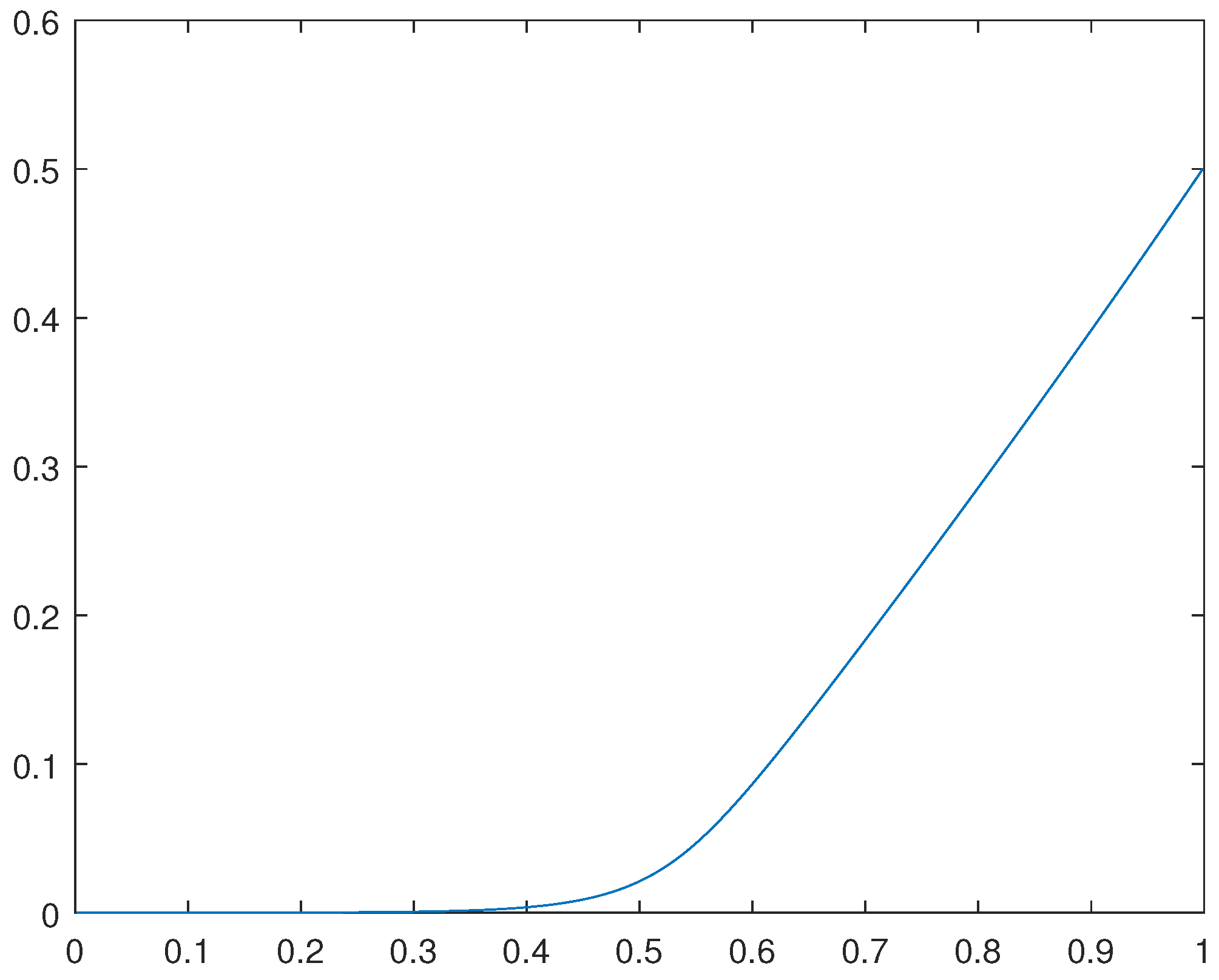
Figure 4.
solution for the case .
Disclaimer/Publisher’s Note: The statements, opinions and data contained in all publications are solely those of the individual author(s) and contributor(s) and not of MDPI and/or the editor(s). MDPI and/or the editor(s) disclaim responsibility for any injury to people or property resulting from any ideas, methods, instructions or products referred to in the content. |
© 2023 by the authors. Licensee MDPI, Basel, Switzerland. This article is an open access article distributed under the terms and conditions of the Creative Commons Attribution (CC BY) license (http://creativecommons.org/licenses/by/4.0/).
Copyright: This open access article is published under a Creative Commons CC BY 4.0 license, which permit the free download, distribution, and reuse, provided that the author and preprint are cited in any reuse.