

Submitted:
23 November 2023
Posted:
23 November 2023
Read the latest preprint version here
Abstract
This article develops duality principles and numerical results for a large class of non-convex variational models. The main results are based on fundamental tools of convex analysis, duality theory and calculus of variations. More specifically the approach is established for a class of non-convex functionals similar as those found in some models in phase transition. Finally, in some sections we present concerning numerical examples and the respective softwares.
Keywords:
duality theory
; non-convex analysis
; numerical method for a non-smooth model
MSC: 49N15; 35A15; 49J40
1. Introduction
In this section we establish a dual formulation for a large class of models in non-convex optimization. It is worth highlighting the main duality principle is applied to double well models similar as those found in the phase transition theory.
Such results are based on the works of J.J. Telega and W.R. Bielski [1–4] and on a D.C. optimization approach developed in Toland [5]. About the other references, details on the Sobolev spaces involved are found in [6]. Related results on convex analysis and duality theory are addressed in [7–13].
Similar models on the superconductivity physics may be found in [14–16].
At this point we recall that the duality principles are important since the related dual variational formulations are either convex (in fact concave) or have a large region of convexity around its critical points. These features are relevant since, from a concerning strict convexity, the standard Newton, Newton type and similar methods are in general convergent. Moreover, the dual variational formulations are relevant since in some situations, from a concerning convexity, it is possible to assure the global optimality of some critical points which satisfy certain specific constraints theoretically established.
Moreover, among the main results, we highlight the duality principles for the quasi-convex formulations in the context of the vectorial calculus of variations. An important example in non-linear elasticity is addressed along the text in details.
Also, for the applications in physics in the final sections, we believe to have found a path to connect the quantum approach with a more classical one in a unified framework.
Indeed, we have presented a path to model a great variety of chemical reactions through such a connection between the atomic and classical worlds.
Finally, in this text we adopt the standard Einstein convention of summing up repeated indices, unless otherwise indicated.
In order to clarify the notation, here we introduce the definition of topological dual space.
Definition 1.1
(Topological dual spaces). Let U be a Banach space. We shall define its dual topological space, as the set of all linear continuous functionals defined on U. We suppose such a dual space of U, may be represented by another Banach space , through a bilinear form (here we are referring to standard representations of dual spaces of Sobolev and Lebesgue spaces). Thus, given linear and continuous, we assume the existence of a unique such that
The norm of f, denoted by , is defined as
At this point we start to describe the primal and dual variational formulations.
2. A general duality principle non-convex optimization
In this section we present a duality principle applicable to a model in phase transition.
This case corresponds to the vectorial one in the calculus of variations.
Let be an open, bounded, connected set with a regular (Lipschitzian) boundary denoted by
Consider a functional where
and where
is a three times Fréchet differentiable function not necessarily convex. Moreover,
and
We assume there exists such that
Furthermore, suppose G is Fréchet differentiable but not necessarily convex. A global optimum point may not be attained for J so that the problem of finding a global minimum for J may not be a solution.
Anyway, one question remains, how the minimizing sequences behave close the infimum of J.
We intend to use duality theory to approximately solve such a global optimization problem.
Denoting
where
, , at this point we define, , , , and by
and
and
Define now ,
Observe that
.
From the general results in [5], we may infer that
On the other hand
From these last two results we may obtain
Moreover, from standards results on convex analysis, we may have
where
and
Thus, defining
we have got
Finally, observe that
This last variational formulation corresponds to a concave relaxed formulation in concerning the original primal formulation.
4. A convex dual variational formulation for a third similar model
In this section we present another duality principle for a third related model in phase transition.
Let and consider a functional where
and where
and
A global optimum point is not attained for J so that the problem of finding a global minimum for J has no solution.
Anyway, one question remains, how the minimizing sequences behave close to the infimum of J.
We intend to use the duality theory to solve such a global optimization problem in an appropriate sense to be specified.
At this point we define, and by
and
Denoting we also define the polar functional and by
and
Observe this is the scalar case of the calculus of variations, so that from the standard results on convex analysis, we have
Indeed, from the direct method of the calculus of variations, the maximum for the dual formulation is attained at some .
Moreover, the corresponding solution is obtained from the equation
Finally, the Euler-Lagrange equations for the dual problem stands for
where if if and
if
We have computed the solutions and corresponding solutions for the cases in which and
For the solution for the case in which , please see Figure 3.
For the solution for the case in which , please see Figure 4.
Remark 4.1.
Observe that such solutions obtained are not the global solutions for the related primal optimization problems. Indeed, such solutions reflect the average behavior of weak cluster points for concerning minimizing sequences.
4.1. The algorithm through which we have obtained the numerical results
In this subsection we present the software in MATLAB through which we have obtained the last numerical results.
This algorithm is for solving the concerning Euler-Lagrange equations for the dual problem, that is, for solving the equation
Here the concerning software in MATLAB. We emphasize to have used the smooth approximation
where a small value for is specified in the next lines.
*************************************
- clear all
- (number of nodes)
-
(we have fixed the number of iterations)
********************************
7. An exact convex dual variational formulation for a non-convex primal one
In this section we develop a convex dual variational formulation suitable to compute a critical point for the corresponding primal one.
Let be an open, bounded, connected set with a regular (Lipschitzian) boundary denoted by
Consider a functional where
and
Here we denote and
Defining
for some appropriate , suppose also F is twice Fréchet differentiable and
Define now and by
and
where here we denote
Moreover, we define the respective Legendre transform functionals and as
where are such that
and
where are such that
Here is any function such that
Furthermore, we define
Observe that through the target conditions
we may obtain the compatibility condition
Define now
for some appropriate such that is convex in
Consider the problem of minimizing subject to
Assuming is large enough so that the restriction in r is not active, at this point we define the associated Lagrangian
where is an appropriate Lagrange multiplier.
Therefore
The optimal point in question will be a solution of the corresponding Euler-Lagrange equations for
From the variation of in we obtain
From the variation of in we obtain
From the variation of in we have
From this last equation, we may obtain such that
and
From this and the previous extremal equations indicated we have
and
so that
and
Replacing the expressions of and into this last equation, we have
so that
Observe that if
then there exists such that u and are also such that
and
The boundary conditions for must be such that
From this and equation (41) we obtain
Summarizing, we may obtain a solution of equation by minimizing on .
Finally, observe that clearly is convex in an appropriate large ball for some appropriate
11. A duality principle for a general vectorial case in the calculus of variations
In this section we develop a duality principle for a general vectorial case in variational optimization.
Let be an open, bounded and connected set with a regular (Lipschitzian) boundary denoted by . Let be a functional where
where
and
Here we have denoted and
so that we may also denote
Assume
where is a differentiable function such that
as . Moreover, suppose there exists such that
It is well known that
Under some mild hypotheses, from convexity, we have that
where
Now observe that the restriction for some is equivalent to the restriction
where , with appropriate boundary conditions, so that with an appropriate Lagrange multiplier , we obtain
where we have denoted
and
Joining the pieces, we have got
where we recall that
We emphasize such a dual formulation in is convex (in fact concave).
12. A note on the Galerkin Functional
Let be an open, bounded and connected set with a regular (Lipschitzian) boundary denoted by .
Consider the functional where
Here ,
We denote also
At this point we define
for some appropriate real constant and
Observe that
so that we define the Galerkin functional by
From this, we get
Define now
At this point, for an appropriate small real constant and bounded constant operator , we set the intended non-active restriction
and define
Observe that since for we have in so that if then
we may infer that is a convex set.
Furthermore, if , then
so that
and hence
For a small parameter we define the intended non-active restriction
and define
Observe that for and sufficiently large is convex in (positive definite Hessian) so that is a convex set. Assuming , define , which is a convex set.
Summarizing, if , then
With such results in mind, we define the following convex optimization problem for finding a critical point of J.
Minimize
subject to
Observe that a critical point of , from such a concerning convexity of on the convex set , is also such that
Finally, we may also define the convex optimization problem of minimizing
subject to
Here is a large real constant.
Such a functional is also convex on so that a critical point of J is also a critical point of , and thus
13. A note on the Legendre-Galerkin functional
Let be an open, bounded and connected set with a regular (Lipschitzian) boundary denoted by .
Consider the functional where
Here ,
We denote also
and , and by
Moreover, we define by
Observe now that these three last suprema are attained through the equations,
From such results, at a critical point, we obtain the following compatibility conditions
From such relations we have
and
so that
and
Moreover, we define the functional by
Therefore
Hence, a critical point of J corresponds to the solution of the following system of equations
and
From this last equation we may obtain
so that the final equations to be solved are
and
with the boundary conditions
With such results in mind, we define the Legendre-Galerkin functional , where
At this point, defining
we obtain
From such results we may infer that
Observe that a critical point so that at a neighborhood of any critical point.
At this point we define
for an appropriate real constant .
Define now ,
for a small real constant
and
Similarly as done in the previous section, we may prove that is a convex set.
Furthermore, for we have that is convex on .
Summarizing, we may define the following convex optimization problem to obtain a critical point of the primal functional J,
We call the Legendre-Galerkin functional associated to J.
13.1. Numerical examples
We have obtained numerical solutions for two one-dimensional examples.
14. A general concave dual variational formulation for global optimization
Let be an open, bounded and connected set a regular (Lipschitzian) boundary denoted by
Consider a functional where
Here , and we also denote
Assume there exists such that
Furthermore, suppose G is three times Fréchet differentiable and there exists such that
Define now where,
where
and
Moreover, we define the polar functionals and , where
and
At this point we define the functional by
With such results in mind we define
and
for appropriated real constants and
Moreover, we define also the penalized functional where
Finally, we remark that for sufficiently small and sufficiently large, is concave in around a concerning critical point. We recall that a critical point
16. One more dual variational formulation
In this section we develop one more dual variational formulation for a related model.
Let and consider the functional defined by
where
We define also the relaxed functional , already including a concerning restriction and corresponding non-negative Lagrange multiplier , where
where
Observe that
Here, we highlight , for some real constant c.
Hence, denoting
and
we have obtained
Finally, for
we emphasize is concave on .
Here is a small regularizing real constant.
Remark 16.1.
The constraint is included to restrict the action of v on the region where the primal functional is non-convex, through an appropriate constant
17. A model in superconductivity through an eigenvalue approach
In this section we intend to model superconductivity through a two phase eigenvalue approach.
Let be a straight wire corresponding to a one-dimensional super-conducting sample.
Consider the functional where
Here, in atomic units, is the total electronic charge, and we set corresponding to higher self-interacting energy which is related to a normal phase. We also set corresponding to a lower self-interacting energy which is related to a super-conducting phase and respective super-currents.
Moreover, we set and initially which is gradually decreased to .
Furthermore, we define
and
where corresponds to a normal phase and to a super-conducting one.
At this point we observe that the temperature is proportional the frequency of vibration for the normal phase.
We start the process with which in atomic units corresponds to a higher temperature and gradually decreases it to the value
Between and the system changes from an almost total normal phase to an almost total super-conducting phase, as expected.
We highlight that the temperature is proportional to the vibrational kinetics energy
so that for
and for a suitable vectorial function , we have
so that we may model the decreasing of temperature T through the decreasing of .
For , for the corresponding normal phase and super-conducting phase , please se Figure 11 and Figure 12, respectively.
For , for the corresponding normal phase and super-conducting phase , please se Figure 13 and Figure 14, respectively.
Finally, we have set which for large corresponds to the super-currents.
18. A simplified qualitative many body model for the hydrogen nuclear fusion
In this section we develop a qualitative simple model for the hydrogen nuclear fusion.
Let be a box in which is confined a gas comprised by an amount of ionized deuterium and tritium isotopes of hydrogen.
Though a suitable increasing in temperature, we intend to develop the following nuclear reaction
We recall that the ionized Deuterium atom comprises a proton and a neutron and the ionized Tritium atom comprises a proton and two neutrons.
Under certain conditions and at a suitable high temperature the ionized Deuterium and Tritium atoms react chemically resulting in an ionized Helium atom, comprised by two protons and two neutrons and resulting also in one more single energetic neutron. We emphasize the higher kinetics neutron energy level has many potential practical applications, including its conversion in electric energy.
At this point we denote by the masses of the ionized Deuterium, Tritium and Helium atoms, and the single neutron, respectively.
Therefore, we have the following mass relation
To simplify our analysis, in such a chemical reaction, denoting the total masses of ionized Deuterium, Tritium, Helium and single Neutrons by and we assume there is a real constant such that
With such statements and definitions in mind, we define the following functional J, where
where, in a simplified many body context,
Here refers to the particle densities.
Furthermore, we assume and , so that
and,
and the kinetics energy is expressed by
where we also assume
so that considering such a vibrational motion, the temperature T is proportional to , that is
Therefore, an increasing in T corresponds to a proportional increasing in
Summarizing, we have supposed
so that we represent the increasing in T through an increasing in
Moreover, we denote by the mass of a single neutron and by the mass of a single proton.
Thus, denoting also by the proportion of non-reacted and reacted masses respectively, we have the following constraints.
Similar constraints are valid corresponding to the charge of a single proton.
We have also the following complementing constraints,
With such results and statements in mind and simplifying the interacting terms, we re-define the functional J now denoting it by , here already including the Lagrange multipliers concerning the constraints, where
where the functional stands for
Remark 18.1.
In order to obtain consistent results it is necessary to set
In such a case, a higher temperature corresponding to a large , though such a nuclear reaction, will result in a small and a higher kinetics energy for the neutron field, corresponding to a large and closer to 1.
19. A more detailed mathematical description of the hydrogen nuclear fusion
In this section we develop in more details another model for the hydrogen nuclear fusion.
Let be an open, bounded and connected set with a regular (Lipschitzian) boundary denoted by
Here such a set stands for a control volume in which an ionized gas (plasma) flows. Such a gas comprises ionized Deuterium and Tritium atoms intended, through a suitable higher temperature, to chemically react resulting in atoms of Hellion and a field of single energetic Neutrons.
Symbolically such a reaction stands for
We recall that the ionized Deuterium atom is comprised by a proton and a neutron and the ionized Tritium atom is comprised by a proton and two neutrons.
Moreover, the ionized Helium atom is comprised by two protons and two neutrons.
As previously mentioned, resulting from such a chemical reaction up surges also an energetic neutron which the higher kinetics energy has a great variety of applications, including its conversion in electric energy.
We highlight the model here presented includes electric and magnetic fields and the corresponding potential ones.
Denoting by t the time on the interval at this point we define the following density functions:
- For the Deuterium field
- For the Tritium field
- For the Helium field
- For the Neutron field
- For the electronic field resulting from the ionization
Furthermore, we define also the related densities
For the chemical reaction in question we consider that one unit of mass of fractional proportion of ionized Deuterium and of ionized Tritium results in one unit of mass of fractional proportion of ionized Helium and of neutrons.
Symbolic, this stands for
Concerning the control volume in question and related surface control we assume such a volume has an initial (fot ) amount of ionized Deuterium of and an initial amount of ionized Tritium of The initial amount of ionized Helium and single neutrons are supposed to be zero.
On the other hand, about the surface control , we assume there is a part for which is allowed the entrance and exit of Deuterium and Tritium ionized atoms.
We assume also there is another part such that for which is allowed only the exit of ionized Helium atoms and neutrons, but not their entrance.
In is allowed the exit only (not the entrance) of ionized Deuterium and Tritium atoms.
Indeed, we assume the following relations for the masses:
-
so that
Here denotes the outward normal vectorial fields to the concerning surfaces.
Having clarified such masses relations, we define the functional
where
and where we assume and , so that
and
and the internal kinetics energy is expressed by
Here it is worth highlighting we have approximated the initially discrete set of indices s of particles as a continuous positive real variable s.
Moreover,
where and are appropriate real constants related to the respective charges.
Here is the fluid velocity field and
are fields of displacements for the corresponding atom fields.
Also denotes the magnetic potential, an external magnetic field and is the total magnetic field.
Moreover, is an induced electric field.
Finally,
for appropriate real positive constants
Such a functional J is subject to the following constraints:
-
The momentum conservation equation for the fluid motionHere is the total density and P is the fluid pressure field.Furthermore,and
- Mass conservation equation:
-
Energy equationwhere we assume the Fourier lawwhere is the scalar field of temperature.Also,and
-
for an appropriate scalar function .
-
Mass relations
- (a)
- (b)
- (c)
- (d)
- (e)
- (f)
- (g)
- (h)
-
so that
where,- (a)
- (b)
- (c)
- (d)
- (e)
- (f)
-
Other mass constraints
- (a)
- (b)
- (c)
- (d)
- (e)
- For the induced electric field, we must havewhere and are appropriate real constants related to the respective charges.
- A Maxwell equation:where
- Another Maxwell equation:where the total electric field stands forand where generically denotingwe have also
At this point we generically denote
Thus, already including the Lagrange multipliers concerning the restrictions indicated, the extended functional stands for
where,
Here we recall the following definitions and relations:
- For the Deuterium field
- For the Tritium field
- For the Helium field
- For the Neutron field
- For the electronic field resulting from the ionization
Also,
-
so that
Finally,
and where generically denoting
we have also
and,
20. A final mathematical description of the hydrogen nuclear fusion
In this section we develop in even more details another model for the hydrogen nuclear fusion.
Let be an open, bounded and connected set with a regular (Lipschitzian) boundary denoted by
Here such a set stands for a control volume in which an ionized gas (plasma) flows. Such a gas comprises ionized Deuterium and Tritium atoms intended, through a suitable higher temperature, to chemically react resulting in atoms of Helium and a field of single energetic Neutrons.
Symbolically such a reaction stands for
We recall that the ionized Deuterium atom is comprised by a proton and a neutron and the ionized Tritium atom is comprised by a proton and two neutrons.
Moreover, the ionized Helium atom is comprised by two protons and two neutrons.
As previously mentioned, resulting from such a chemical reaction up surges also an energetic neutron which the higher kinetics energy has a great variety of applications, including its conversion in electric energy.
We highlight the model here presented includes electric and magnetic fields and the corresponding potential ones.
Denoting by t the time on the interval at this point we define the following density functions:
- For a single Deuterium atom indexed by s:
- For a single Tritium atom indexed by s:
- For a single Helium atom indexed by s:
- For the Neutron field:
- For the electronic field resulting from the ionization
Furthermore, we define also the related densities
For the chemical reaction in question we consider that one unit of mass of fractional proportion of ionized Deuterium and of ionized Tritium results in one unit of mass of fractional proportion of ionized Helium and of neutrons.
Symbolically, this stands for
Concerning the control volume in question and related surface control we assume such a volume has an initial (fot ) amount of ionized Deuterium of and an initial amount of ionized Tritium of The initial amount of ionized Helium and single neutrons are supposed to be zero.
On the other hand, about the surface control , we assume there is a part for which is allowed the entrance and exit of Deuterium and Tritium ionized atoms.
We assume also there is another part such that for which is allowed only the exit of ionized Helium atoms and neutrons, but not their entrance.
In is allowed the exit only (not the entrance) of ionized Deuterium and Tritium atoms.
Indeed, we assume the following relations for the masses:
-
so that
- Here denotes the outward normal vectorial fields to the concerning surfaces.
Having clarified such masses relations, denoting by the respective indexed number of particles at time t, we define the functional
where
and where we assume and , so that
and
and the internal kinetics energy is expressed by
Moreover,
where and are appropriate real constants related to the respective charges.
Here is the fluid velocity field and
are fields of displacements for the corresponding particle fields.
Also denotes the magnetic potential, an external magnetic field and is the total magnetic field.
Moreover, is an induced electric field.
Also,
for appropriate real positive constants
Finally,
where are small real positive constants.
Such a functional J is subject to the following constraints:
-
The momentum conservation equation for the fluid motionHere is the total density and P is the fluid pressure field.Furthermore,and
- Mass conservation equation:
-
Energy equationwhere we assume the Fourier lawwhere is the scalar field of temperature.Also,and
-
for an appropriate scalar function .
-
Mass relations
- (a)
- (b)
- (c)
- (d)
- (e)
where,- (a)
- (b)
- (c)
- (d)
- (e)
- (f)
- (g)
-
so that
- (h)
- (i)
-
Other mass constraints
- (a)
- (b)
- (c)
- (d)
- (e)
- (f)
- (g)
- (h)
- For the induced electric field, we must havewhere and are appropriate real constants related to the respective charges.
- A Maxwell equation:where
- Another Maxwell equation:where the total electric field stands forand where generically denotingwe have also
At this point we generically denote
Thus, already including the Lagrange multipliers concerning the restrictions indicated, the extended functional stands for
where,
Here we recall the following definitions and relations:
- For the Deuterium field
- For the Tritium field
- For the Helium field
- For the Neutron field
- For the electronic field resulting from the ionization
Also,
-
so that
Finally,
and where generically denoting
we have also
and,
21. A qualitative modeling for a general phase transition process
In this section we develop a general qualitative modeling for a phase transition process.
Let be an open, bounded and connected set with a regular (Lipschitzian) boundary denoted by
Such a set is supposed to a be a fixed volume in which an amount of mass of a substance A with a density function u will develop phase a transition for another phase with corresponding density function The total mass is suppose to be kept constant throughout such a process.
We model such transition in phase through a functional where
Here and
The phases corresponding to u and v are connected through a Lagrange multiplier E, which represents the chemical potential of the chemical process in question.
We assume the temperature is directly proportional to the internal kinetics energy where
For a internal vibrational motion, we assume approximately
for an appropriate frequency and vectorial function
Thus, the temperature is indeed proportional to , that is, symbolically, we may write
Therefore, we start with the system with a phase corresponding to and at . Gradually increasing the temperature to a corresponding , we obtain a transition to a phase corresponding to and .
At this point, we also define the index normalized corresponding densities
and
Finally, we have obtained some numerical results for the following parameters:
, ,
-
We start with corresponding to and in .
-
We end the process with corresponding to and in .
22. A mathematical description of a hydrogen molecule in a quantum mechanics context
In this section we develop a mathematical description for a hydrogen molecule.
Let be an open, bounded and connected set with a regular (Lipschitzian) boundary denoted by .
Observe that a single hydrogen molecule comprises two hydrogen atoms physically linked through their electrons.
We recall that each hydrogen atom comprises one proton, one neutron and one electron.
Since the electric charge interaction effects are much higher than those related to the respective masses, in a first analysis we neglect the single neutron densities.
Denoting and time , generically, for a particle at the atom in the molecule , we define the following general density:
Here we have the particle density in the atom with density , at the molecule with a global density .
Here we have also denoted, the particle mass, the mass of atom and the mass of molecule , so that we set the following constraints:
At this point we denote for the atoms e of a hydrogen molecule:
- : mass of electron in the atom , where
- : mass of proton in the atom , where
Therefore, considering the respective indexed densities for the particles in question, we define the total hydrogen molecule density, denoted by as
Such system is subject to the following constraints:
- From the proton in the atom :
- For the proton in the atom :
- For the atom :
- For the atom :
- For the electrons and , concerning the physical electronic link between the atoms:
- For the total molecular density:
Therefore, already including the Lagrange multipliers, the corresponding variational formulation for such a system stands for , where
Here we denote
we assume
and
Finally,
Remark 22.1.
We highlight the two electrons which link the atoms are at same level of energy . Morever, each atom has its energy level and the molecule as a whole has also its energy level
23. A mathematical model for the water hydrolysis
In this section we develop a modeling for a chemical reaction known as the water hydrolysis.
Let be an open, bounded and connected set with a regular (Lipschitzian) boundary denoted by
In such a volume containing a total mass of water initially at the temperature 25 C with pressure 1 atm, we intend to model the following reaction
which as previously mentioned is the well known water hydrolysis.
We highlight stand for a water molecule which subject to an appropriate electric potential is decomposed into a ionized molecule and ionized atom.
It is also well known that the water symbol corresponds to a molecule with two hydrogen (H) atoms and one oxygen (O) atom.
Moreover, the oxygen atom O has 8 protons, 8 neutrons and 8 electrons whereas the hydrogen atom H has one proton, one neutron and one electron.
Remark 23.1.
Here we have assumed that a unit mass of reacts into a fractional mass of and a fractional mass of
Symbolically, we have:
To clarify the notation we set the conventions:
- molecule generically corresponds to wave function .
- molecule corresponds to wave function
- hydrogen atom corresponds to wave function
At this point we define the following densities:
- For the water density (for charges), denoted by , we havewhere is the mass of a single water molecule and generically refers to the hydrogen proton at the hydrogen atom concerning the molecular density and so on.
- For the density, denoted by , we havewhere is the mass of a single molecule of .
- For the ionized hydrogen atom have
where we have denoted is the mass of a single atom of .
Here and are appropriate real constants concerning a proton and an electron charge, respectively.
The system is subject to the following constraints:
Already including the Lagrange multipliers for the constraints, the variational formulation for such system. denoted by the functional stands for
where
Here , , , , ,
Moreover,
where , , and
Furthermore,
where is an electric potential originated from an external electric field applied on
Finally,
24. A mathematical model for the Austenite and Martensite phase transition
In this section we consider a phase transition of a solid solution of () and carbon with a proportion of carbon, known as austenite, initially at a temperature above and close to and rapidly cooled to a temperature of about , developing a phase transition which generates a solid solution of () and carbon known as martensite.
Let be an open, bounded and connected set with a regular boundary denoted by which contains an amount of austenite at and which, as previously mentioned, is rapidly cooled to a temperature on a time interval resulting a phase known as martensite.
We recall the of austenite phase presents a multi-faced cubic crystalline structure in a micro-structure with carbon atoms.
On the other hand, structure of the martensite phase has a cubic centralized crystalline structure in a micro-structure with carbon atoms.
At this point, we also recall that the (iron) atom has 26 protons, 26 electrons and 30 neutrons.
On the other hand a atom has 6 protons and this same number of electrons and neutrons.
Here we define the density function , representing the Austenite phase, where:
Similarly, we define the density function for the Martensite phase, which is denoted by , where:
For the corresponding to the Austenite phase, such density functions are subject to the following constraints:
Defining
and
we must have
where is a small real parameter related to crystalline structure dimensions.
We must have also,
and,
For the corresponding to the Austenite phase, such density functions are subject to the following constraints:
Defining
we must have
where is a small real parameter related to crystalline structure dimensions.
We must have also,
The other constraints for the densities are given by:
-
For the Austenite phase:
- (a)
- (b)
- (c)
- (d)
- (e)
- (f)
- (g)
- (h)
-
For the Martensite phase:
- (a)
- (b)
- (c)
- (d)
- (e)
- (f)
- (g)
- (h)
- For the total (iron) mass,
- For the total Carbon mass
At this point we define the functional J which models such a pahse transition in question, where
where
Also,
Finally, , where
and,
Finally, for a field of displacements resulting from the action of a external load field and temperature variations, we define
where
and
Remark 24.1.
The system temperature is supposed to be directly proportional to , which in this model is a known function obtained experimentally. Finally, the strain tensors and refer to austenite and martensite phases, respectively. Such tensors also depend on the temperature and must be also obtained experimentally.
25. A note on classical free fields through a variational perspective
This section is strongly based on the first chapter of the book [20], by N.N. Bogoliubov and D.V. Shirkov.
Therefore, the credit for this section is of these mentioned authors. This section is a kind of review of such a book chapter indicated. In fact, what we have done is simply to open more and clarify some calculations, specially about the first variation of the functional L, in order to improve their understanding.
Let where is a bounded, open and connected set with a regular boundary denoted by
Consider the Lagrangian density and an action where
.
We denote
and
Assume is such that
so that
We define a change of variables
where and (here t denotes time).
Also
where denotes a small real parameter.
We define also
where
and
Observe that
so that
Summarizing, we have got
Define now
where we have generically denoted
and
From such a last definition we have
so that
At this point we define
so that
From this and
we obtain
In particular, for
and
we obtain
Moreover, we define
so that
In particular, for
and
we obtain the Energy-Momentum tensor , where
25.1. The Angular-Momentum tensor
In this subsection we define the following change of variables
where
With such relations in mind, we set
We define also,
where
Moreover, we define
where
Hence,
For the general variation, we define again
where we have generically denoted
and
Moreover, we set
and
Thus,
so that
With such results in mind, we define
Similarly as in the previous section, we may obtain
Thus,
where
so that
where
and
The tensor is said to be the Orbital angular momentum tensor and is said to be Spin one.
26. A note on quantum field operators
This section is strongly based on the chapter 3, page 53 of the book [21], by G.B. Folland.
Therefore, here we have done a kind of review of these pages of such a book chapter indicated. In fact, we have simply opened more and clarified some calculations, in order to improve their understanding.
Let where is a open, bounded and connected set with a regular boundary denoted
Define and
Consider an operator where in a distributional sense,
and where
Suppose there exists operators and such that
and
Assume also is such that
and
Now define
Observe that
We shall prove by induction that
Indeed, for
so that (150) holds for .
Suppose now (150) holds for so that
In order to complete the induction, it suffices to prove that (150) holds for
Observe that
Thus, the induction is complete, so that
Moreover, we recall that
so that
Summarizing, we have got
Now, we shall prove that
Observe that
Summarizing, we have got
so that
Finally, from such results, we may infer that
Similarly,
Therefore we have got
that is
Thus, for each , is an eigenvalue of H with corresponding eigenvector .
26.1. An application concerning the harmonic oscillator operator in quantum mechanics
In this section we have the aim of representing the relativistic Klein-Gordon equation through the creation and annihilation operations related to the harmonic oscillator in quantum mechanics.
Consider first the one-dimensional Hamiltonian, corresponding to the harmonic oscillator, namely
which through an appropriate re-scale results into the following related Hamiltonian , where
Define now the operators
and
Clearly,
so that
Similarly, as in the previous sections, by induction, we may obtain
For
we define
Also from the previous section, we may obtain
and
so that
Here we recall that
and
In reference [21], page 54 it is proven that such a sequence is an ortho-normal basis for
Finally, observe that for we may define
and
Here generically,
Observe that clearly
and
Denoting where t stands for time, consider the relativistic Klein-Gordon equation,
From the previous results, we may represent such an equation by
We highlight from the previous results we know the action of and on an appropriate basis of obtained though an appropriate tensorial product of the bases
We shall call the operators and as the creation and annihilation operators concerning the original harmonic operator in quantum mechanics.
To justify such a nomenclature, we recall that and
28. The generalized method of lines applied to fourth order differential equations
In this sections we develop an application of the generalized method of lines to a fourth order equation.
We start by addressing the following ordinary differential equation (ode):
with the boundary conditions
and
In terms of linear elasticity, such a boundary conditions corresponds to a bi-clamped beam.
In a finite difference context, this last equation corresponds to
where N is the number of nodes and .
Considering that, from the boundary conditions, for we get
so that
where
Similarly, for , we obtain
Hence, replacing the value of previously obtained in this last equation, we have
so that
where defining , we have also
Now reasoning inductively, for n, having
and
we obtain
so that from this and
we obtain
so that
where defining
we obtain
and
Summarizing, we have got
Observe now that from the boundary conditions,
From these last two equations, we may obtain
and
and so on up to obtaining
The problem is then solved.
28.1. A numerical example
We develop a numerical example considering
and
Thus, we have solved the equation
with the boundary conditions
and
In a finite differences context, we have used nodes and
For a solution , please see Figure 19.
In the next lines, we present the concerning software in MAT-LAB
**************
-
clear allm8=100;d=1/m8;e1=1.0;for i=1:m8f(i,1)=1.0;end;a(1)=2/3;b(1)=-1/6;c(1)=f(1,1)*/(6e1);m12=(6-4*a(1));a(2)=(4*b(1)+4)/m12;b(2)=-1/m12;c(2)=1/m12*(4*c(1)+f(2,1)*/e1);for i=3:m8-2m12=(a(i-2)*a(i-1)+b(i-2)-4*a(i-1)+6);a(i)=-1/m12*(a(i-2)*b(i-1)-4*b(i-1)-4);b(i)=-1/m12;c(i)=1/m12*(f(i,1)*/e1-c(i-2)-a(i-2)*c(i-1)+4*c(i-1));end;u(m8,1)=0;u(m8-1,1)=0;for i=2:m8-1;u(m8-i,1)=a(m8-i)*u(m8-i+1,1)+b(m8-i)*u(m8-i+2,1)+c(m8-i);end;for i=1:m8x(i)=i*d;end;plot(x,u)******************
29. Applications to the optimal shape design for a beam model
In this section, we present a numerical procedure for the shape optimization concerning the Bernoulli beam model.
Let corresponds to the horizontal axis of a straight beam with rectangular cross section , that is, the beam has a variable thickness distributed along such a horizontal axis x, where
Define now
which corresponds to a simply supported beam.
Consider the problem of minimizing in the functional
subject to
where
is variable beam thickness, corresponds to a rectangular cross section perpendicular to the x axis, and E is the young elasticity model.
Also, we define
where and
Observe that
where
Summarizing, we have got
In order to obtain numerical results, we suggest the following primal dual procedure:
- Set and
- Calculate solution of equationwhere
- Calculate such thatwhere
- Set and go to step 2 until an appropriate convergence criterion is satisfied.
We have developed numerical results for , , , , and
We have also defined
where
For the optimal solution , please see Figure 20.
For a corresponding optimal solution , please see Figure 21.
Remark 29.1.
For such a simply-supported beam model, for the numerical solution of equation
with the boundary conditions
firstly we have solved the equation
with the boundary conditions
Subsequently, we have solved the equation
with the boundary conditions
Here we present the software developed in MAT-LAB.
******************
-
clear allglobal m8 d d2wo H e1 ho h1 xo b5m8=100;d=1.0/m8;b5=0.1;e1=210*;ho=0.18;A=zeros(m8-1,m8-1);for i=1:m8-1A(1,i)=1.0;xo(i,1)=0.55;x3(i,1)=0.55;end;lb=0.4*ones(m8-1,1);ub=ones(m8-1,1);b=zeros(m8-1,1);b(1,1)=0.65*(m8-1);for i=1:m8f(i,1)=1.0;L(i,1)=1/2;P(i,1)=36.0*;end;i=1;m12=2;m50(i)=1/m12;z(i)=1/m50(i)*(-P(i,1)*);for i=2:m8-1m12=2-m50(i-1);m50(i)=1/m12;z(i)=m50(i)*(-P(i,1)*+z(i-1));end;v(m8,1)=0;for i=1:m8-1v(m8-i,1)=m50(m8-i)*v(m8-i+1,1)+z(m8-i);end;k=1;b12=1.0;while andkk=k+1;for i=1:m8-1H(i,1)=b5*/12*e1;f1(i,1)=v(i,1)/H(i,1);end;i=1;m12=2;m70(i)=1/m12;z1(i)=m70(i)*(-f1(i,1)*);for i=2:m8-1m12=2-m70(i-1);m70(i)=1/m12;z1(i)=m70(i)*(-f1(i,1)*+z1(i-1));end;w(m8,1)=0;for i=1:m8-1w(m8-i,1)=m70(m8-i)*w(m8-i+1,1)+z1(m8-i);end;d2wo(1,1)=(-2*w(1,1)+w(2,1))/;for i=2:m8-1d2wo(i,1)=(w(i+1,1)-2*w(i,1)+w(i-1,1))/;end;k9=1;b14=1.0;whilek9k9=k9+1;X=fmincon(’beamNov2023’,xo,A,b,,lb,ub);b14=max(abs(xo-X))xo=X;end;b12=max(abs(xo-x3))x3=xo;for i=1:m8-1L(i,1)=xo(i,1);end;end;***************
With the auxiliary function "beamNov2023":
********************
-
function S=beamNov2023(x)global m8 d d2wo H e1 ho h1 xo b5S=0;for i=1:m8-1S=S+1//b5/e1*(H(i,1)**12;end;*****************************
We develop numerical results also for
Such boundary conditions corresponds to bi-clamped beam. The remaining data is equal to the previous example
For the optimal solution , please see Figure 22.
For a corresponding optimal solution , please see Figure 23.
Remark 29.2.
For such a bi-clamped beam model, for the numerical solution of equation
with the boundary conditions
firstly we have solved the equation
with the boundary conditions
Subsequently, we solved the equation
with the boundary conditions
obtaining such that the boundary conditions
are also satisfied.
Here we present the software developed in MAT-LAB.
*************************
-
clear allglobal m8 d d2wo H e1 ho h1 xo b5m8=100;d=1.0/m8;b5=0.1;e1=210*;ho=0.18;A=zeros(m8-1,m8-1);for i=1:m8-1A(1,i)=1.0;xo(i,1)=0.55;x3(i,1)=0.55;end;lb=0.4*ones(m8-1,1);ub=ones(m8-1,1);b=zeros(m8-1,1);b(1,1)=0.65*(m8-1);for i=1:m8f(i,1)=1.0;L(i,1)=1/2;P(i,1)=36.0*;end;i=1;m12=2;m50(i)=1/m12;z(i)=1/m50(i)*(-P(i,1)*);for i=2:m8-1m12=2-m50(i-1);m50(i)=1/m12;z(i)=m50(i)*(-P(i,1)*+z(i-1));end;v(m8,1)=0;for i=1:m8-1v(m8-i,1)=m50(m8-i)*v(m8-i+1,1)+z(m8-i);end;k=1;b12=1.0;whilekk=k+1;for i=1:m8-1H(i,1)=b5*/12*e1;f1(i,1)=v(i,1)/H(i,1);f2(i,1)=i*d/H(i,1);f3(i,1)=1/H(i,1);end;i=1;m12=2;m70(i)=1/m12;z1(i)=m70(i)*(-f1(i,1)*);z2(i)=m70(i)*(-f2(i,1)*);z3(i)=m70(i)*(-f3(i,1)*);for i=2:m8-1m12=2-m70(i-1);m70(i)=1/m12;z1(i)=m70(i)*(-f1(i,1)*+z1(i-1));z2(i)=m70(i)*(-f2(i,1)*+z2(i-1));z3(i)=m70(i)*(-f3(i,1)*+z3(i-1));end;w1(m8,1)=0;w2(m8,1)=0;w3(m8,1)=0;for i=1:m8-1w1(m8-i,1)=m70(m8-i)*w1(m8-i+1,1)+z1(m8-i);w2(m8-i,1)=m70(m8-i)*w2(m8-i+1,1)+z2(m8-i);w3(m8-i,1)=m70(m8-i)*w3(m8-i+1,1)+z3(m8-i);end;m3(1,1)=w2(1,1);m3(1,2)=w3(1,1);m3(2,1)=w2(m8-1,1);m3(2,2)=w3(m8-1,1);h3(1,1)=-w1(1,1);h3(2,1)=-w1(m8-1,1);h5(:,1)=inv(m3)*h3;for i=1:m8wo(i,1)=w1(i,1)+h5(1,1)*w2(i,1)+h5(2,1)*w3(i,1);end;d2wo(1,1)=(-2*wo(1,1)+wo(2,1))/;for i=2:m8-1d2wo(i,1)=(wo(i+1,1)-2*wo(i,1)+wo(i-1,1))/;end;k9=1;b14=1.0;whilek9k9=k9+1;X=fmincon(’beamNov2023’,xo,A,b,,lb,ub);b14=max(abs(xo-X))xo=X;end;b12=max(abs(xo-x3))x3=xo;for i=1:m8-1L(i,1)=xo(i,1);end;end;*****************************
Remark 29.3.
About the numerical results obtained for these two beam models, a final word of caution is necessary.
Indeed, the full convergence in such cases is hard to obtain so that we have obtained just approximations of critical points with the functionals close to their optimal values. It is also worth emphasizing we have fixed the number of iterations so that the solutions and shapes obtained are just approximate ones.
30. Applications to the optimal shape design for a plate model
In this section, we present a numerical procedure for the shape optimization concerning a thin plate model.
Let corresponds to the middle surface of a thin plate with a variable thickness .
Define now
which corresponds to a simply supported plate.
Consider the problem of minimizing in the functional
subject to
where
is variable plate thickness, E is the young elasticity model and .
Also, we define
where and
Observe that
where
Summarizing, we have got
In order to obtain numerical results, we suggest the following primal dual procedure:
- Set and
- Calculate solution of equationwhere
- Calculate such thatwhere
- Set and go to step 2 until an appropriate convergence criterion is satisfied.
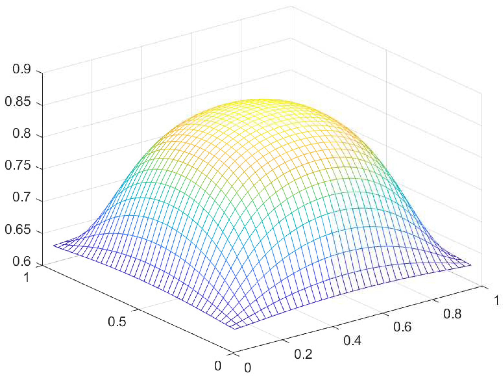
We have developed numerical results for , , , and
We have also defined
where
For the optimal solution , please see Figure 24.
For a corresponding optimal solution , please see Figure 25.
Remark 30.1.
For such a simply-supported plate model, for the numerical solution of equation
with the boundary conditions
firstly we have solved the equation
with the boundary conditions
Subsequently, we have solved the equation
with the boundary conditions
Here we present the software developed in MAT-LAB.
*********************
-
clear allglobal m8 d d2xwo d2ywo H e1 ho xo b5m8=40;d=1.0/m8;w5=0.3;e1=200*/;ho=0.12;A=zeros();for i=1:A(1,i)=1.0;xo(i,1)=0.55;x3(i,1)=0.55;end;lb=0.45*ones(,1);ub=ones(,1);b=zeros(,1);b(1,1)=0.75*for i=1:(m8-1)for j=1:m8-1f(i,j,1)=1.0;L(i,j,1)=1/2;P(i,j,1)=2*; end;end;for i=1:m8wo(:,i)=0.001*ones(m8-1,1);end;m2=zeros(m8-1,m8-1);for i=2:m8-2m2(i,i)=-2.0;m2(i,i-1)=1.0;m2(i,i+1)=1.0;end;m2(1,1)=-2.0;m2(1,2)=1.0;m2(m8-1,m8-1)=-2.0;m2(m8-1,m8-2)=1.0;Id=eye(m8-1);i=1;m12=2*Id-m2*; m50(:,:,i)=inv(m12);z(:,i)=m50(:,:,i)*(-P(:,i,1)*);for i=2:m8-1m12=2*Id-m2*-m50(:,:,i-1);m50(:,:,i)=inv(m12);z(:,i)=m50(:,:,i)*(-P(:,i,1)*+z(:,i-1));end; v(:,m8)=zeros(m8-1,1);for i=1:m8-1v(:,m8-i)=m50(:,:,m8-i)*v(:,m8-i+1)+z(:,m8-i);end;k=1;b12=1.0;while () and ()kk=k+1;for i=1:m8-1for j=1:m8-1H(j,i,1)=/12*e1;f1(j,i,1)=v(j,i)/H(j,i,1);end;end;i=1;m12=2*Id-m2*;m70(:,:,i)=inv(m12);z1(:,i)=m70(:,:,i)*(-f1(:,i,1)*);for i=2:m8-1m12=2*Id-m2*-m70(:,:,i-1);m70(:,:,i)=inv(m12);z1(:,i)=m70(:,:,i)*(-f1(:,i,1)*+z1(:,i-1));end;w(:,m8)=zeros(m8-1,1);for i=1:m8-1w(:,m8-i)=m70(:,:,m8-i)*w(:,m8-i+1)+z1(:,m8-i);end;d2xwo(:,1)=(-2*w(:,1)+w(:,2))/;for i=2:m8-1d2xwo(:,i)=(w(:,i+1)-2*w(:,i)+w(:,i-1))/;end;for i=1:m8-1d2ywo(:,i)=m2*w(:,i)/;end;k9=1; b14=1.0;while () and ()k9k9=k9+1;X=fmincon(’beamNov2023A3’,xo,A,b,,lb,ub);b14=max(abs(xo-X))xo=X;end;b12=max(max(abs(w-wo)))wo=w;x3=xo;for i=1:m8-1for j=1:m8-1L(j,i,1)=xo((i-1)*(m8-1)+j,1);end;end;end;for i=1:m8-1x8(i,1)=i*d;end;mesh(x8,x8,L);*********************
With the auxiliary function "beamNov2023A3’, where
****************************
-
function S=beamNov2023A3(x)global m8 d d2xwo d2ywo H e1 ho xo b5S=0;for i=1:m8-1for j=1:m8-1x1(j,i)=x((m8-1)*(i-1)+j,1);end;end;for i=1:m8-1for j=1:m8-1S=S+;end;end;********************************
Remark 30.2.
About the numerical results obtained for this plate model, a final word of caution is necessary.
Indeed, the full convergence in such a case is hard to obtain so that we have obtained just approximations of critical points with the functional close to its optimal value. It is also worth emphasizing we have fixed the number of iterations so that the solution and shape obtained are just approximate ones.
31. A note on the first Maxwell equation of electromagnetism
Let be an open, bounded and connected set with a regular (Lipschitzian) boundary denoted by .
Suppose is an electric field of class in
Let be also an open, bounded and connected set with a regular (Lipschitzian) boundary denoted by .
Observe that the exists a scalar field such that
and
Here denotes the normal outward field to S.
Observe also that
so that defining
we have that
Hence, from such results and the divergence Theorem, we get
Summarizing, we have got
Consider now a charge localized at the center of a sphere of radius and boundary
The electric field on the sphere surface generated by is given by
where is the normal outward field to .
Clearly
Consider again the set but now with a charge localized at a point inside the interior of , which is denoted by .
At first the electric field generated by is not of class on
However, there exists such that
Define .
Therefore, is of class on
Denoting the boundary of by , from the previous results, we may infer that
so that
Therefore, we have got
Assume now on we have a density of charges .
For a small volume consider a punctual charge localized in such that
Denoting by the electric field generated by , from the previous results we may infer that
Such an equation in its differential form, stands for:
Integrating in we may obtain
so that
From this and the Divergence Theorem, we have
Summarizing, we have got
This is the integral form of the first Maxwell equation of electromagnetism.
For this last equation, the set is rather arbitrary so that for as a ball of small radius with center at a point , from the Mean Value Theorem fot integrals and letting , we obtain
This last equation stands for the differential form of the first Maxwell equation of electromagnetism.
Remark 31.1.
Summarizing, in this section we have formally obtained a mathematical deduction of the first Maxwell equation of electromagnetism.
32. Conclusion
In the first part of this article we have developed a relaxation proposal and duality principles suitable for a large class of models in physics and engineering.
In a second part we develop duality principles for the quasi-convex envelop of some vectorial models in the calculus of variations.
We highlight such dual variational formulations established are in general convex (in fact concave).
Finally, in the last sections, we develop mathematical models for some types of chemical reactions, including the hydrogen nuclear fusion and the water hydrolysis. Among such results, we highlight our proposal of modeling the Ginzburg-Landau theory in super-conductivity as a two-phase eigenvalue approach.
Data Avaliability
Details on the software for numerical results avaialable upon request.
e-mail: fabio.botelho@ufsc.br
Conflict of interest declaration
The author declares no conflict of interest concerning this article.
References
- Bielski, W.R.; Galka, A.; Telega, J.J. The Complementary Energy Principle and Duality for Geometrically Nonlinear Elastic Shells. I. Simple case of moderate rotations around a tangent to the middle surface. Bull. Pol. Acad. Sci. Tech. Sci. 1988, 38, 7–9. [Google Scholar]
- Bielski, W.R.; Telega, J.J. A Contribution to Contact Problems for a Class of Solids and Structures. Arch. Mech. 1985, 37, 303–320. [Google Scholar]
- Telega, J.J. On the complementary energy principle in non-linear elasticity. Part I: Von Karman plates and three dimensional solids. Part II: Linear elastic solid and non-convex boundary condition. Minimax approach, ibid. C.R. Acad. Sci. Paris Serie II 1989, 308, 1193–1198. [Google Scholar]
- Galka, A.; Telega, J.J. Duality and the complementary energy principle for a class of geometrically non-linear structures. Part I. Five parameter shell model; Part II. Anomalous dual variational priciples for compressed elastic beams. Arch. Mech. 1995, 47, 677–698. [Google Scholar]
- Toland, J.F. A duality principle for non-convex optimisation and the calculus of variations. Arch. Rat. Mech. Anal. 1979, 71, 41–61. [Google Scholar] [CrossRef]
- Adams, R.A.; Fournier, J.F. Sobolev Spaces, 2nd ed.; Elsevier: New York, NY, USA, 2003. [Google Scholar]
- Botelho, F. Functional Analysis and Applied Optimization in Banach Spaces; Springer: Cham, Switzerland, 2014. [Google Scholar]
- Botelho, F.S. Functional Analysis, Calculus of Variations and Numerical Methods in Physics and Engineering; CRC Taylor and Francis: Boca Raton, FL, USA, 2020. [Google Scholar]
- Botelho, F.S. Variational Convex Analysis. Ph.D. Thesis, Virginia Tech, Blacksburg, VA, USA, 2009. [Google Scholar]
- Botelho, F. Topics on Functional Analysis, Calculus of Variations and Duality; Academic Publications: Sofia, Bulgaria, 2011. [Google Scholar]
- Botelho, F. Existence of solution for the Ginzburg-Landau system, a related optimal control problem and its computation by the generalized method of lines. Appl. Math. Comput. 2012, 218, 11976–11989. [Google Scholar] [CrossRef]
- Rockafellar, R.T. Convex Analysis; Princeton University Press: Princeton, NJ, USA, 1970. [Google Scholar]
- Botelho, F.S. Dual Variational Formulations for a Large Class of Non-Convex Models in the Calculus of Variations. Mathematics 2023, 11, 63. [Google Scholar] [CrossRef]
- Annet, J.F. Superconductivity, Superfluids and Condensates, 2nd ed.; Oxford Master Series in Condensed Matter Physics; Oxford University Press: Oxford, UK, 2010. [Google Scholar]
- Landau, L.D.; Lifschits, E.M. Course of Theoretical Physics, Vol. 5-Statistical Physics, Part 1; Elsevier Butterworth-Heinemann: Oxford, UK, 2008. [Google Scholar]
- Botelho, F.S. Advanced Calculus and its Applications in Variational Quantum Mechanics and Relativity Theory; CRC Taylor and Francis: Boca Raton, FL, USA, 2021. [Google Scholar]
- Ciarlet, P. Mathematical Elasticity, Vol. II—Theory of Plates; Elsevier: North Holland, The Netherlands, 1997. [Google Scholar]
- Attouch, H.; Buttazzo, G.; Michaille, G. Variational Analysis in Sobolev and BV Spaces; MPS-SIAM Series in Optimization; Society for Industrial and Applied Mathematics: Philadelphia, PA, USA, 2006. [Google Scholar]
- Strikwerda, J.C. Finite Difference Schemes and Partial Differential Equations, 2nd ed.; SIAM: Philadelphia, PA, USA, 2004. [Google Scholar]
- Bogoliubov, N.N.; Shirkov, D.V. Introduction of the Theory of Quantized Fields, Monographs and Texts in Physics and Astronomy; Intercience Publishers INC.: New York, NY, USA, 1959; Volume 3. [Google Scholar]
- Folland, G.B. Quantum Field Theory, A Tourist Guide for Mathematicians, Mathematical Surveys and Monographs; Americam Mathematical Society, AMS: Providence, RI, USA, 2008; Volume 149. [Google Scholar]
Figure 1.
solution for the case .
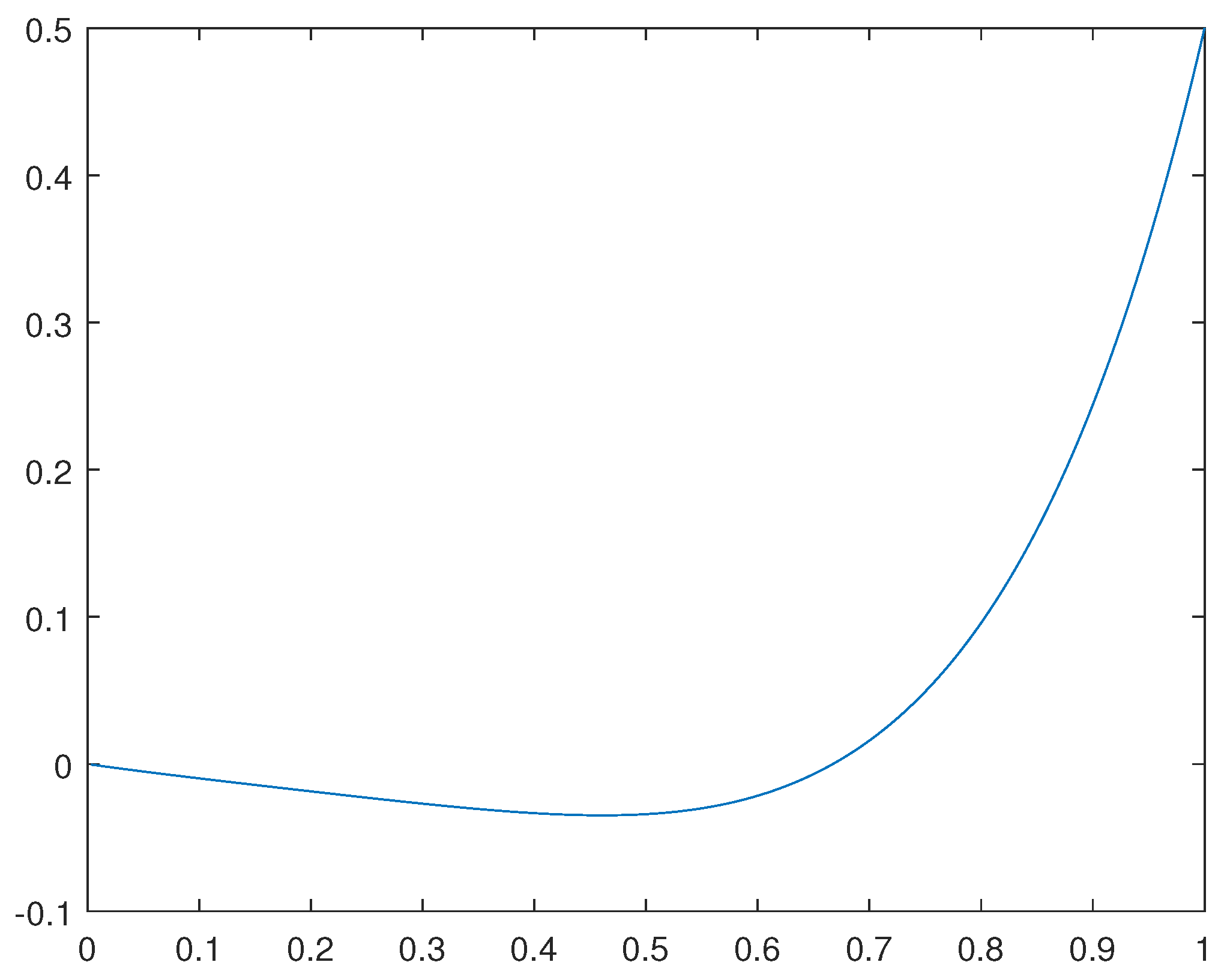
Figure 2.
solution for the case .
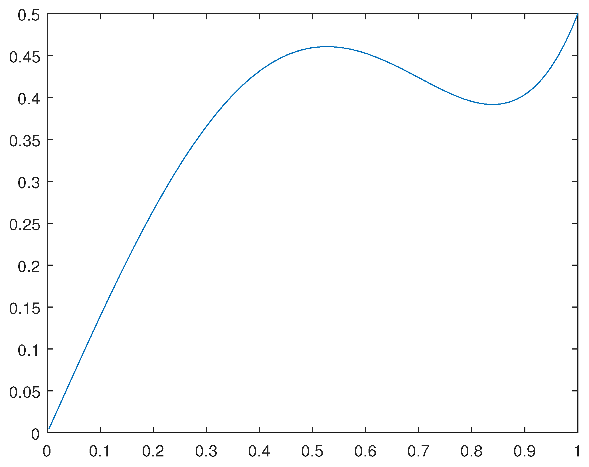
Figure 3.
solution for the case .
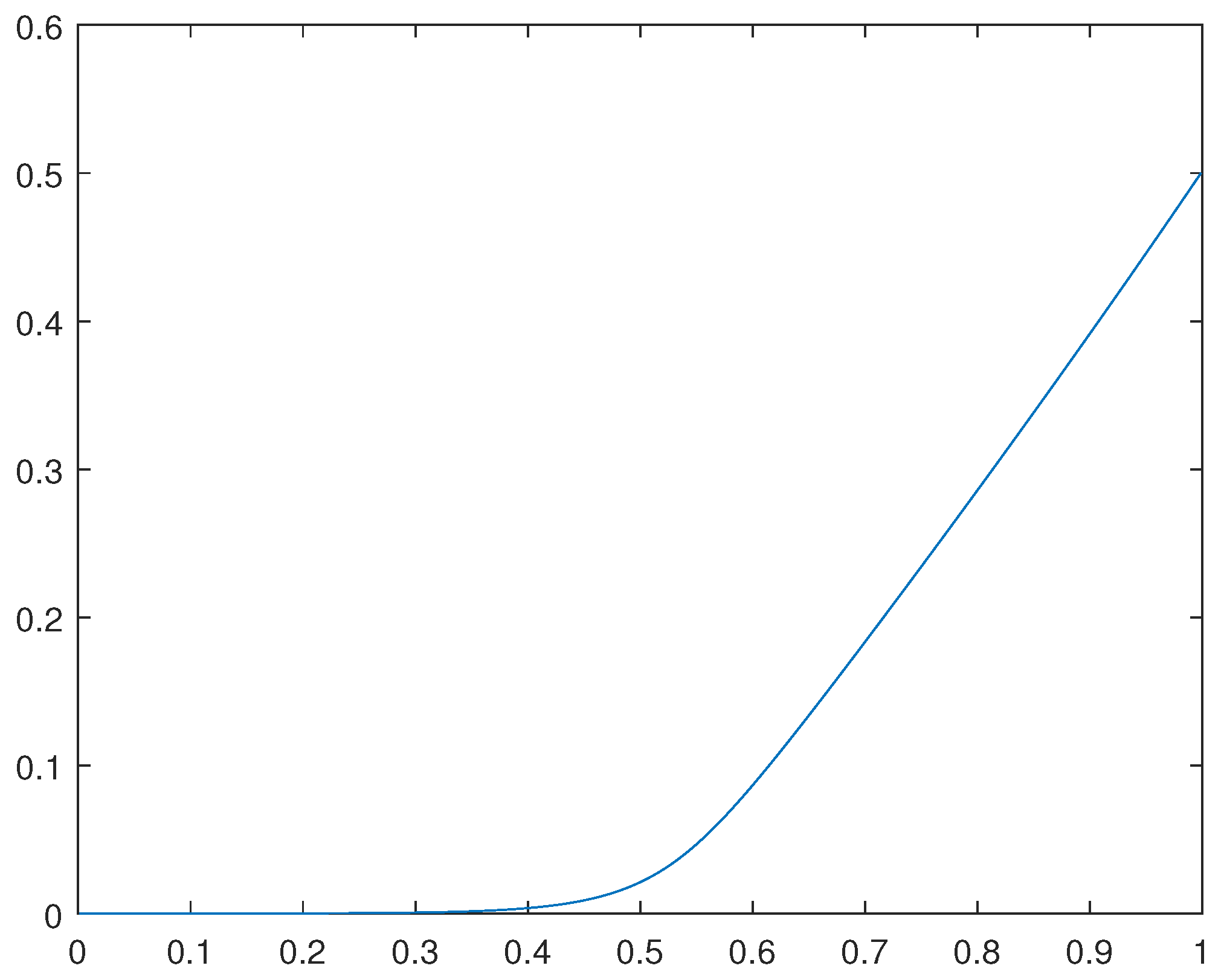
Figure 4.
solution for the case .
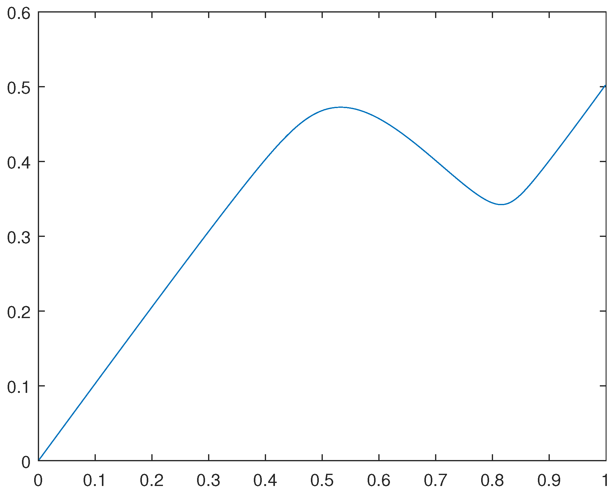
Figure 5.
Density for the Case A.

Figure 6.
Density for the Case B.

Figure 7.
Solution for the example 1.
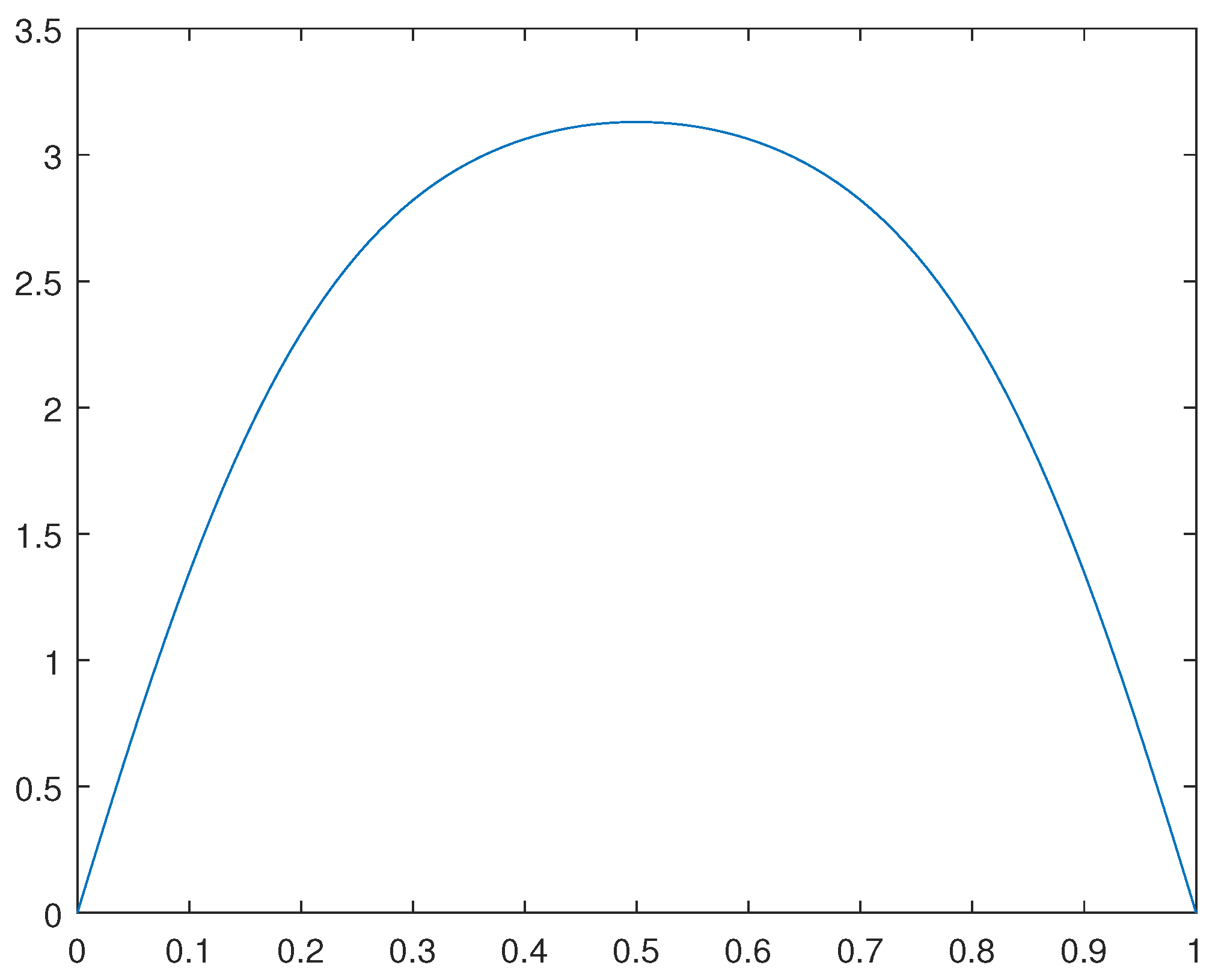
Figure 8.
Solution for the example 2.
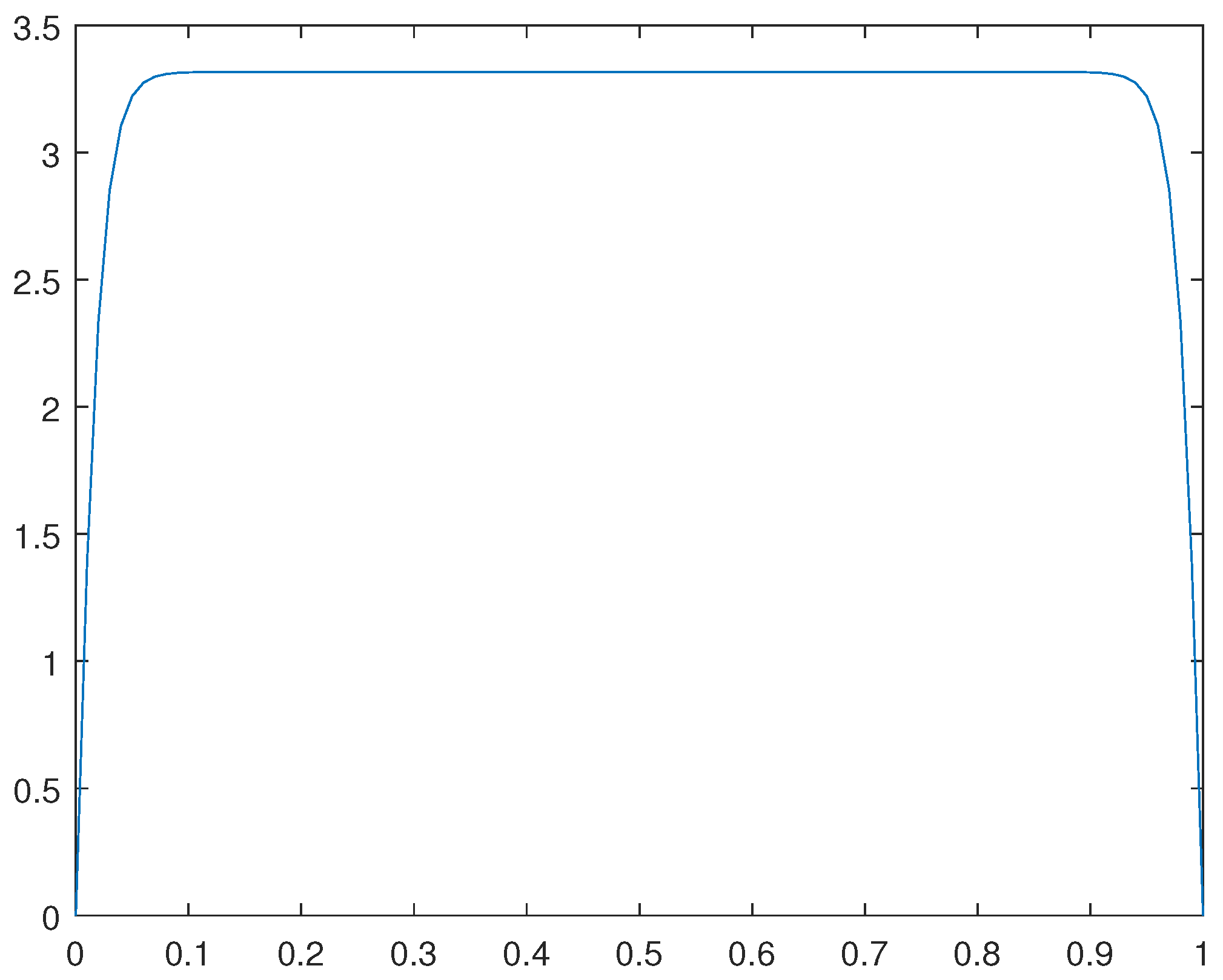
Figure 9.
Solution for the example A.
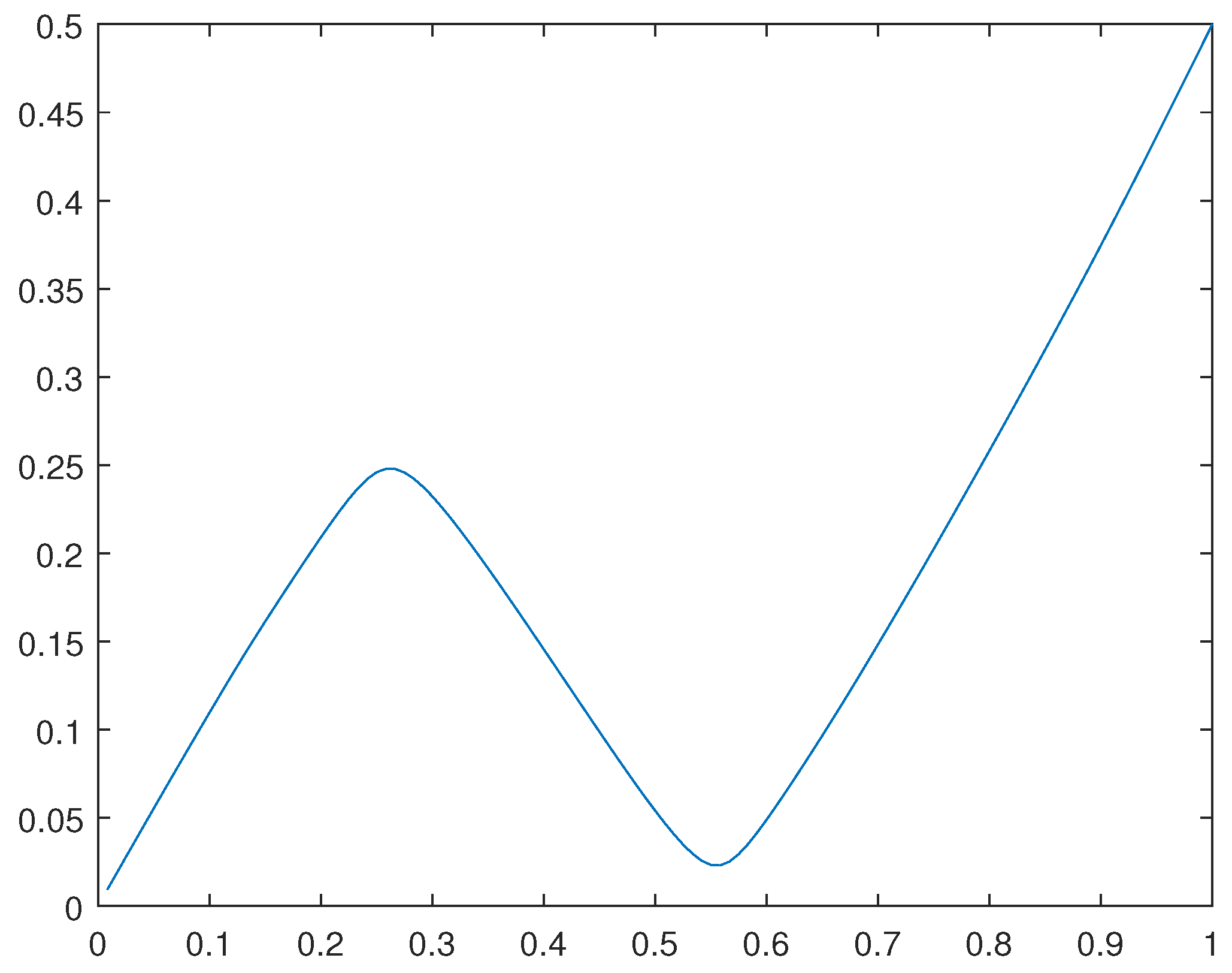
Figure 10.
Solution for the example B.
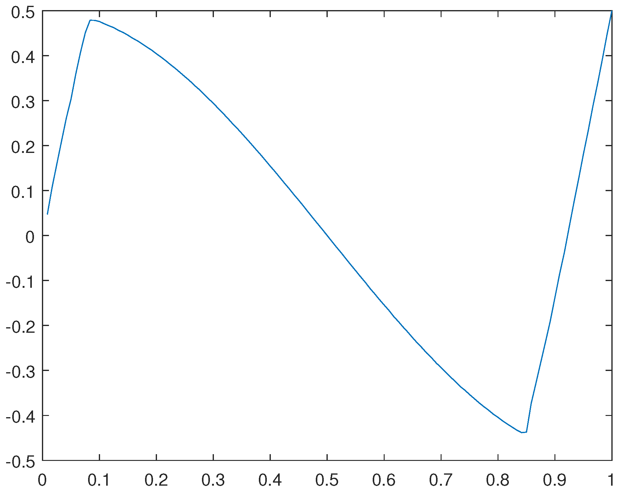
Figure 11.
Solution for the .
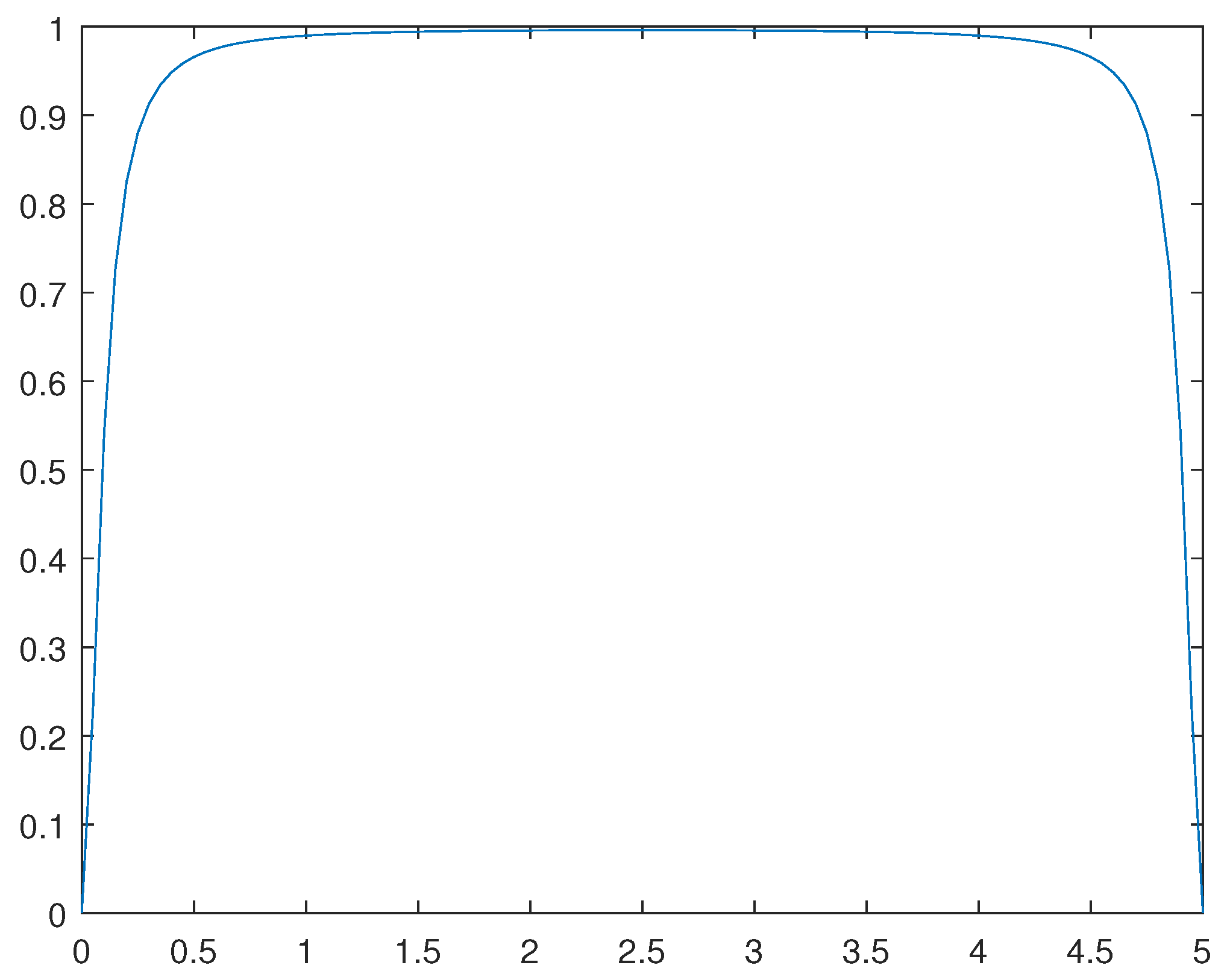
Figure 12.
Solution for the .
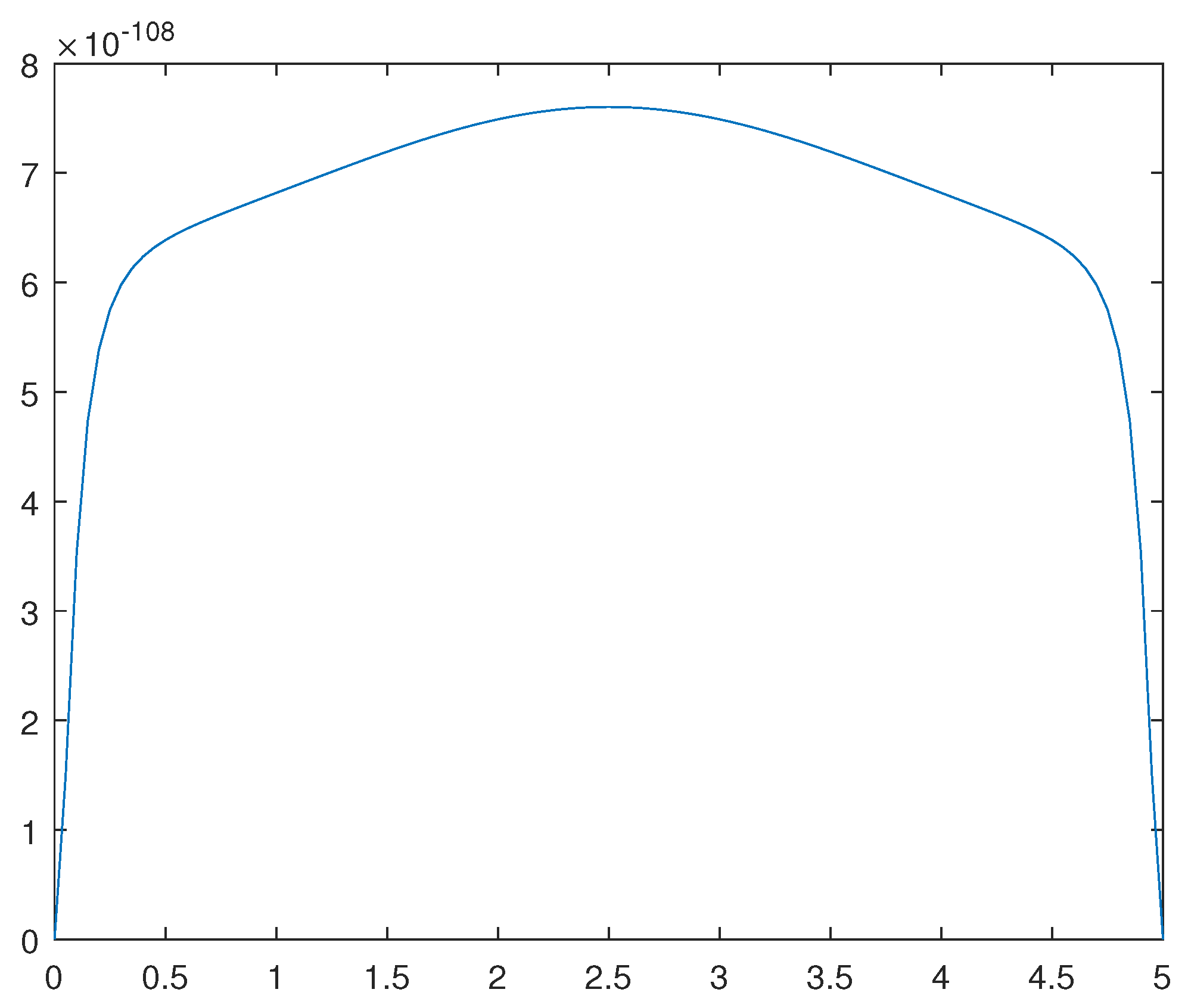
Figure 13.
Solution for the .
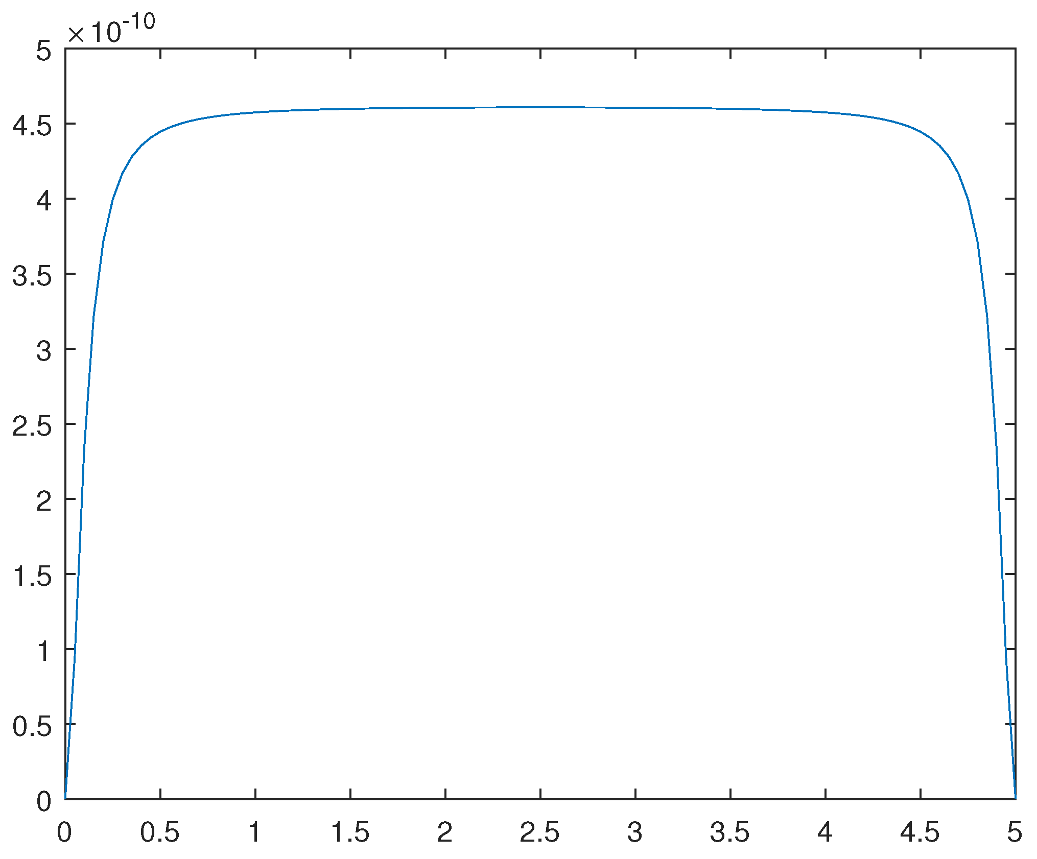
Figure 14.
Solution for the .
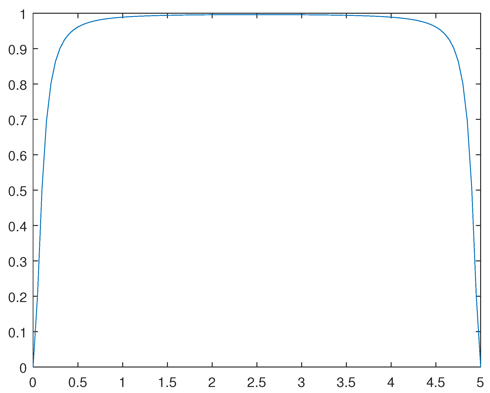
Figure 15.
Solution for .
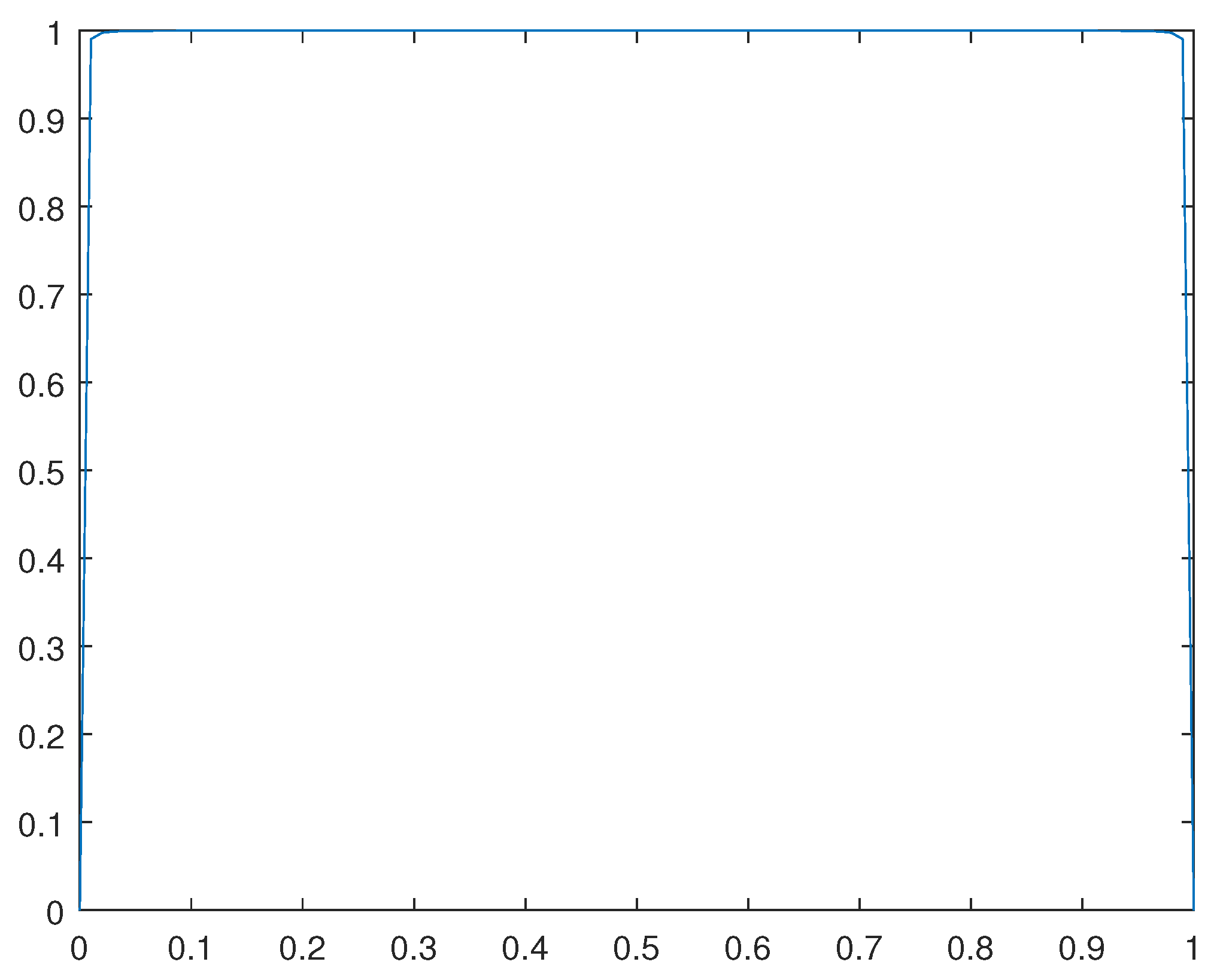
Figure 16.
Solution for .
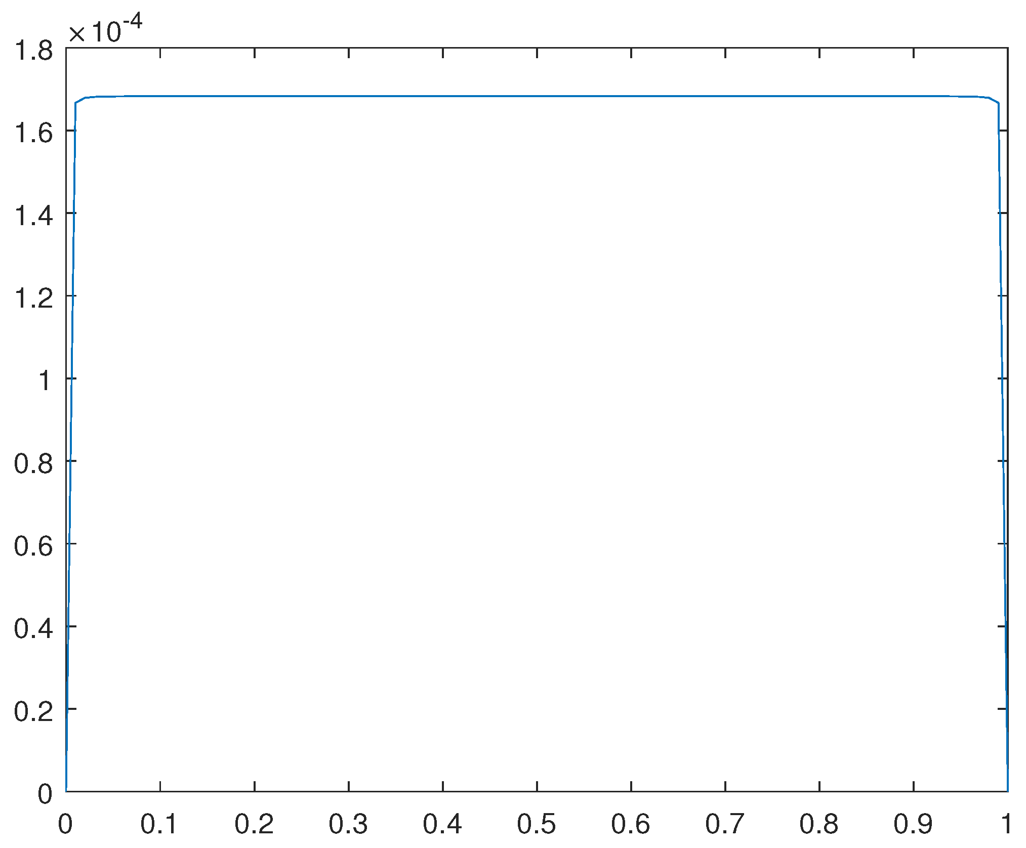
Figure 17.
Solution for .
Figure 18.
Solution for .
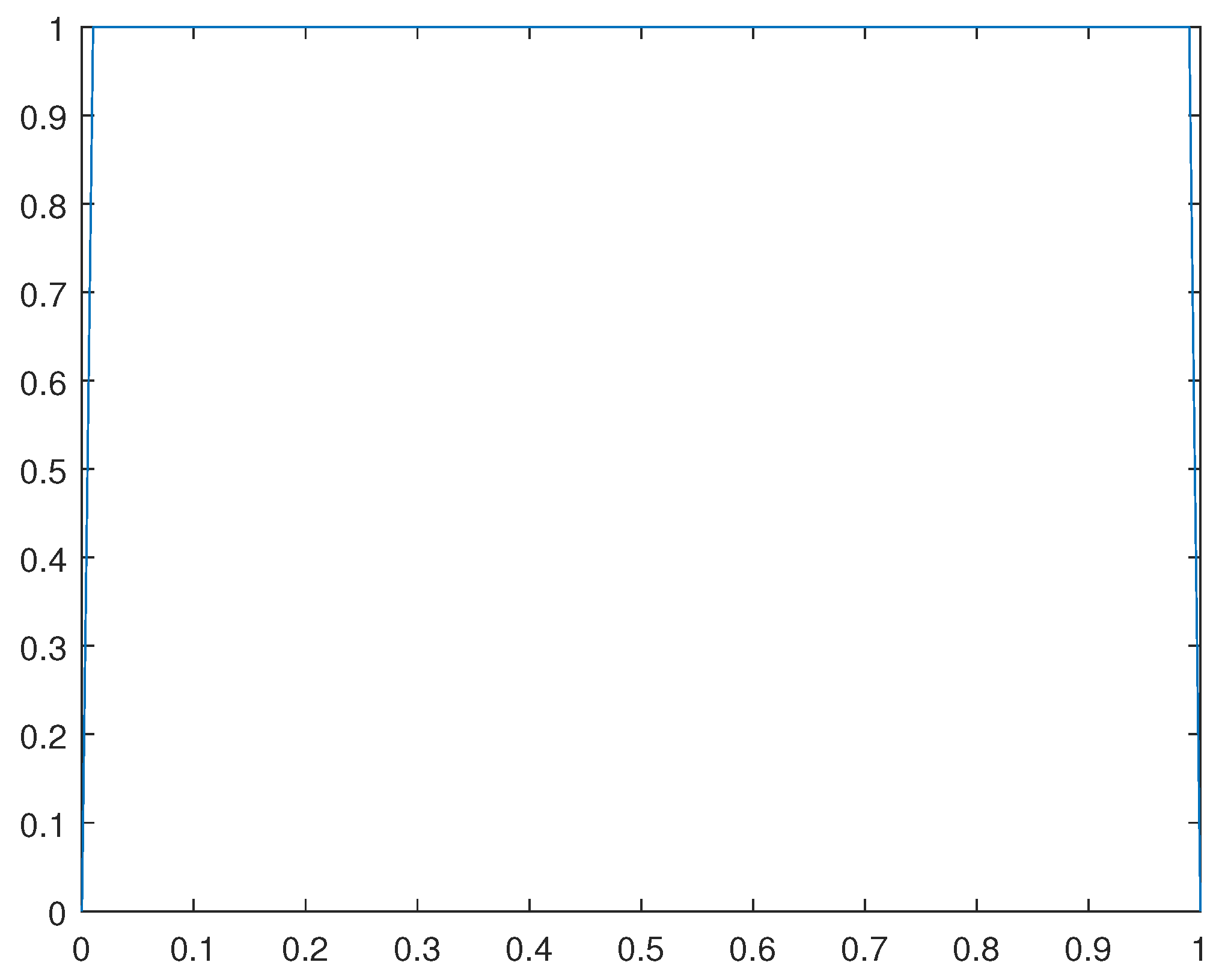
Figure 19.
Solution for the example B.
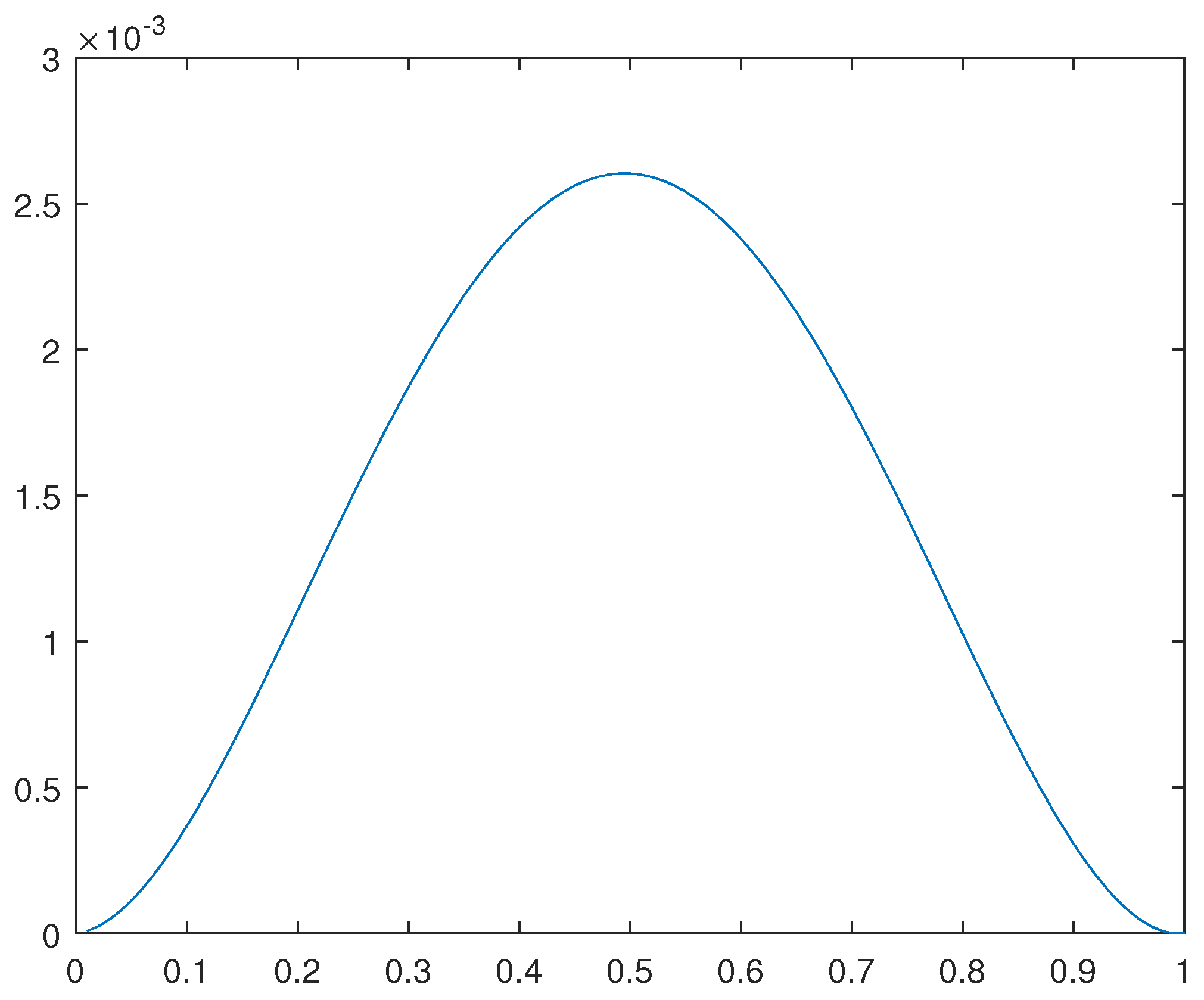
Figure 20.
Optimal solution for a simply supported beam.
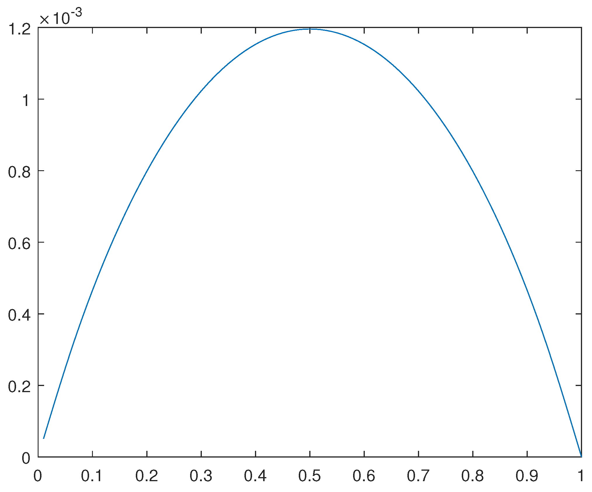
Figure 21.
Optimal shape solution for a simply supported beam.
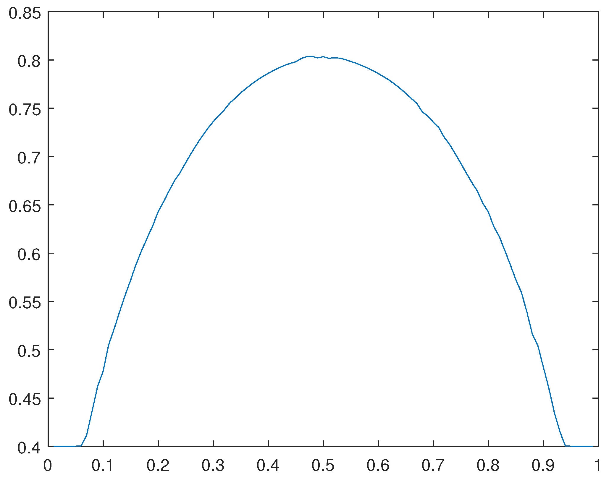
Figure 22.
Optimal solution for a bi-clamped beam.
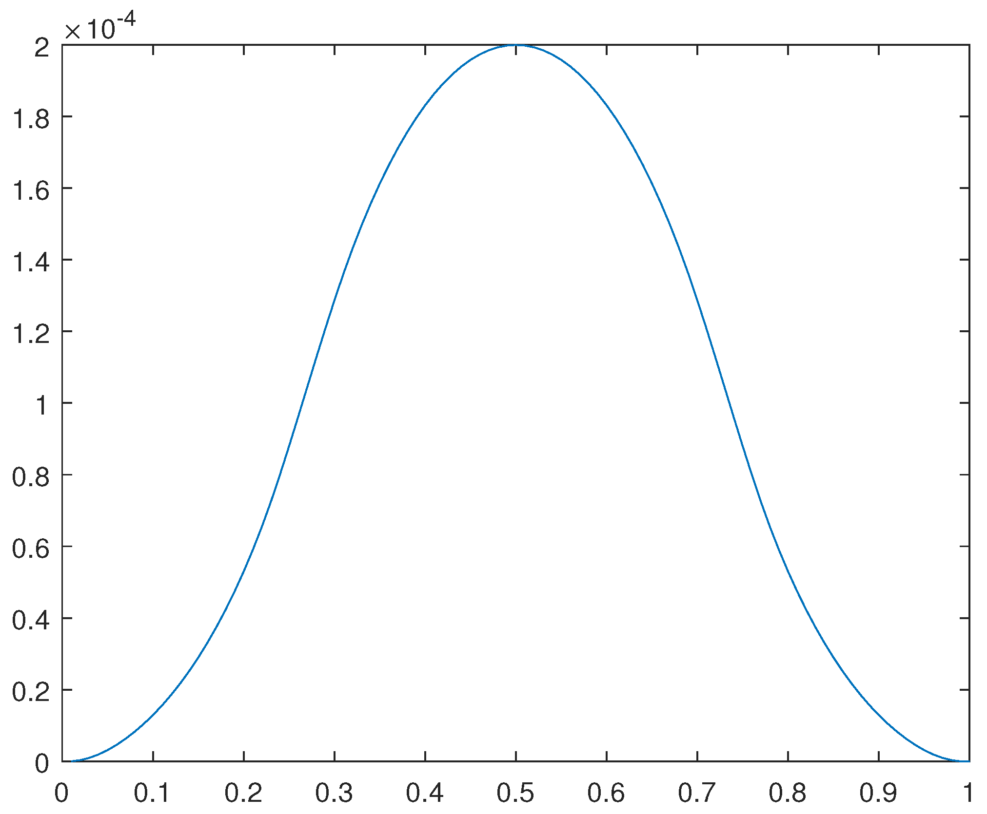
Figure 23.
Optimal shape solution for a bi-clamped beam.
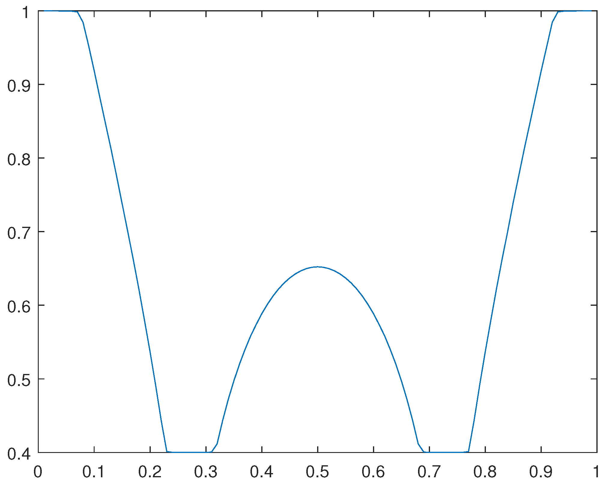
Figure 24.
Optimal solution for a simply supported plate.
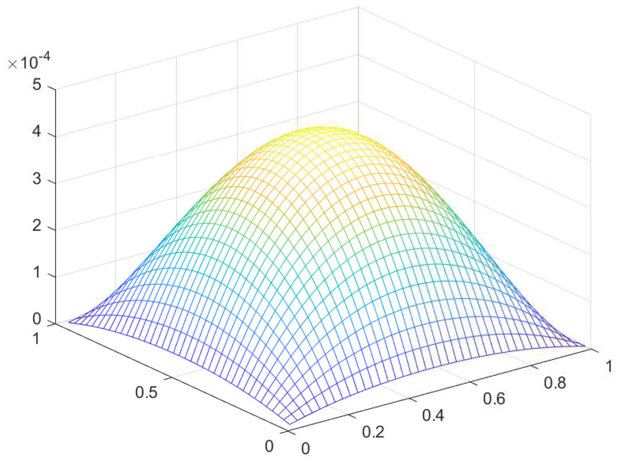
Figure 25.
Optimal shape solution for a simply supported plate.
Disclaimer/Publisher’s Note: The statements, opinions and data contained in all publications are solely those of the individual author(s) and contributor(s) and not of MDPI and/or the editor(s). MDPI and/or the editor(s) disclaim responsibility for any injury to people or property resulting from any ideas, methods, instructions or products referred to in the content. |
© 2023 by the authors. Licensee MDPI, Basel, Switzerland. This article is an open access article distributed under the terms and conditions of the Creative Commons Attribution (CC BY) license (http://creativecommons.org/licenses/by/4.0/).
Copyright: This open access article is published under a Creative Commons CC BY 4.0 license, which permit the free download, distribution, and reuse, provided that the author and preprint are cited in any reuse.