
Submitted:
13 January 2023
Posted:
16 January 2023
You are already at the latest version
Abstract
Clew Bay is an important aquaculture production area in Ireland. In this study, we focused on a high-resolution simulation of the Clew Bay region based on a Regional Ocean Modelling System (ROMS). Freshwater discharges from eight rivers are included in the model and a wetting-drying scheme has been implemented. The Clew Bay model simulation was validated and calibrated with available observations (e.g., Acoustic Doppler Current Profilers (ADCP), vertical salinity and temperature profiles and tide gauge) in the geographic area of the model domain. High correlations were found between the model outputs and observed temperature, salinity and tide gauge water levels along with small Root Mean Square Errors. This indicates that the model was able to reproduce the oceanographic phenomena in the study area. The Taylor diagram analysis showed a high correlation coefficient (R=0.99) between the ADCP bottom temperature in the Inner Bay and the Clew Bay model, along with a small Centered Root Mean Square Error (RMSD =0.5 ◦ C). High correlation coefficients (R > 0.80) were found between the model and the two ADCPs for the zonal current component. There was a resemblance in structure between the model and the observed salinity profiles, indicating that freshwater was correctly implemented in the model. Moreover, the correlation coefficient between the model and the tidal sea surface height (SSH) was 0.99, with an RMSD of 0.09 m. We discovered that wind direction and speed have a significant impact on the bay's water inflow rate. The model outputs can be used to provide scientists, fishermen and decision-makers with hydrodynamic information on ocean conditions in the bay.
Keywords:
Clew Bay
; ROMS
; ADCP
; Tide Gauge
; Taylor Diagram
; SSH
1. Introduction
Clew Bay is a large bay with an area of about 176 km2 (i.e., 16 km from east to west and 11 km from north to south) situated on the west coast of Ireland, characterized by a large number of islands (see Fig. 1). The bay is bounded by Croagh Patrick Mountains to the south and Achill Island to the north (Fig. 1). The islands in Clew Bay are partially drowned drumlins, i.e., elongated, steeply sloping hills that were sometimes called “whalebacks” [1]. They were formed when glaciers reshaped the landscape during the last ice age [1]. Several of the hills on the mainland around the bay are similar drumlins [2]. These glacial formations vary considerably in size, ranging from large islands on which residences and pastures stand to small mounds on the seafloor [1]. The numerous islands give rise to shallow straits and lagoons through which deep channels flow [2]. Erosion of existing and submerged drumlins with their coarse glacial deposits gives rise to a heterogeneous sediment environment [2,3]. Clew Bay has three hundred and sixty-five islands, the largest one, Clare Island, protects the entrance to the sheltered bay [4], as shown in Figure 1.
Clew Bay is an important national region responsible for aquaculture (i.e., finfish farming, oysters farming, mussels, and others) industry in Ireland [5]. In 2020, there were 22 aquaculture-related businesses in Clew Bay [6], the vast majority of which were involved in oyster farming, although shellfish and finfish farming are also represented locally https://bim.ie/wp-content/uploads/2022/05/Clew-Bay-Report-SPREADS.pdf. Finfish and oyster farming extends from the Westport River to the Burrishoole Fishery (Loughs Feagh and Furnace) near Newport and is an important national region [6] (Figure 1).
There is a need for hindcasts and forecasts of hydrodynamic properties for the Clew Bay region by a wide range of stakeholders, e.g., scientists working on salmon migration. To date, there are no published modeling studies for Clew Bay.
As regards other recent modelling studies of Irish waters, the set-up and validation results of a high-resolution numerical operational model developed at the Irish Marine Institute covering the northeast Atlantic with emphasis on Irish waters were presented in [7]. The model is based on ROMS with a horizontal resolution of 1 km and runs operationally. The meanders and eddies in the model domain were well resolved. The authors attribute this to the high resolution of the model and detailed bathymetry in the study area. In addition, [8] has presented a high-resolution (1 km) 3-D ocean model based on ROMS for southwestern Irish waters. The simulation of the Irish hindcast model was validated and calibrated with available observations in the geographic domain of the model. The model has been shown to be robust when compared to CTD vertical temperature and salinity profiles.
Furthermore, in [9], a 3D model of the coastal ocean was created using simple equations for Bantry Bay. The model was developed, validated, and implemented operationally.
The authors have found some other modeling studies of the Irish shelf waters, e.g. [10,11,12,13,14,15,16,17,18,19]. Moreover, in [20] preliminary results of a high-resolution 3D numerical simulation with a wetting and drying scheme based on the Regional Ocean Modelling System (ROMS) were used to study the tidal circulation in Kilmakiloge Harbour. This bay is located on the southern shore of Kenmare Harbour. The model showed good skill and a high correlation coefficient with respect to the available observations, especially for temperature and tides. However, the model overestimated mixing in Kilmakilloge Harbour.
To the best of the authors knowledge, the presented model is the first 3D numerical model developed for Clew Bay. This study reports the validation results of the preoperational model. The model was initialized on June 7, 2017, and ran until January 1, 2019. The model has a horizontal resolution of 80 m and 15 vertical sigma levels. The model was validated using currents recorded by an Acoustic Doppler Current Profiler (ADCP), temperature and salinity profiles from the Irish Environmental Protection Agency (EPA) Ireland website, and water level records from a tide gauge. The Clew Bay net flow and residence time were estimated. Section 2 describes the model implementation and nesting procedures. Section 3 presents the validation against observational data, describes the general circulation in the Clew Bay region, estimates of the net flow and residence time, and discusses the results before presenting the conclusions in the last section.
2. Model Design, Description and Implementation
The model is based on version 3.7 of the code Regional Ocean Modelling System [21]. All model equations are written in rectangular coordinates and include spatially and temporally varying horizontal eddy viscosity and diffusion coefficients [22]. The Clew Bay model has a horizontal grid with a resolution of 80x80 meters and 15 vertical sigma layers. The high-resolution bathymetry of the Clew Bay model is from Ireland's Integrated Mapping for the Sustainable Development of Ireland's Marine Resource (INFOMAR) database (www.infomar.ie; downloaded on June 19, 2022) and the European Marine Observation and Data Network (EMODnet) bathymetric dataset (https://www.emodnet-bathymetry.eu/). Minimal smoothing of the bathymetry was performed using a linear programming method [23]. The model also has a wetting and drying scheme according to [24]. The scheme specifies that some points of the ocean grid may be completely “wet” or “dry”. These “dry” points may not have zero depth; instead, they are covered by a thin film of water so that the equations of motion can be calculated at all grid points [25]. The direction of flow is determined at each of the faces of a tracer cell, and the flow and velocity through the face are set to zero if the depth of the upstream tracer cell is less than or equal to a user-specified critical depth Dcrit [24,25]. The authors set the Dcrit to 0.25 m. The turbulence mixing scheme of the model is a k-ε parameterization implemented by the Generic Length Scale (GLS) scheme [26,27]. An upstream third-order scheme with implicit mixing was used for the horizontal advection of momentum [28], whilst multidimensional positive definite advection transport algorithm (MPDATA) was used for horizontal and vertical advection of tracers [29]. Bottom stress is applied using the logarithmic “wall law” with a constant roughness length of 0.01 m.
The Marine Institute's operational model for the Northeast Atlantic (NEA_ROMS) provides the initial conditions for the Clew Bay model of the three open boundaries [7]. The initial and boundary parameters of the model include temperature, salinity, baroclinic and barotropic velocity components, and sea surface height. The temporal resolution of the boundary conditions is 10 minutes and includes the tidal signal. The nesting was designed so that the volume transport across the open boundary of the nested model matches the volume transport of the NEA _ROMS model; this technique was described in [7].
The atmospheric data for the computation of the surface forcing are taken from the global high resolution (0.125o) atmospheric model run by the European Centre for Medium Range Weather Forecasts (ECMWF) at a 3 -hour frequency. The atmospheric fields used are air temperature, relative humidity, wind speed at 10 m above sea level, mean sea level pressure, cloud cover, total precipitation, and solar radiation (surface and net longwave). Wind stress, heat fluxes, and evaporation rates are calculated using an interactive mass formula that uses atmospheric data, as described in [8]. Daily averaged freshwater discharges were specified for eight major freshwater sources (see Table 1). Data for four rivers were obtained from the European Hydrological Forecasts for the Environment (Swedish Meteorological and Hydrological Institute (E-HYPE SMHI)); https://hypeweb.smhi.se/explore-water/historical-data/europe-time-series/) [30], while the remaining rivers were obtained from the Irish Environmental Protection Agency (EPA) Ireland website. . Daily climatological flows for the four rivers in the E- HYPE (Owenwee, Burrishole, Owengrave, and Mayour) were calculated from available flow time series over a 30-year period (1981 - 2010). Daily flow rates for the Newport, Westport, Owennabrockagh, and Bunowen rivers were determined from time series from EPA for a 10-year period (2006-2016). Salinity of incoming freshwater was set to zero, and temperature was calculated from monthly temperatures for the period 2000-2010, available at HYPE-SMHI: (https://hypeweb.smhi.se/explore-water/historical-data/europe-time-series/).
The model was initialized on June 7, 2017 and ran until January 1, 2019. The output consists of temperature, salinity, sea surface height, barotropic, and baroclinic velocity fields and is stored in netCDF files in hourly snapshots. In addition, the output is stored at a frequency of 10 minutes at selected locations in the area for use in model validation.
Data used to validate the 1.5 year hindcast simulation (i.e., June 2017–1st January 2019), included two ADCPs, four EPA temperature and salinity profiles and Roonagh Tide Gauge Station (see Figure 1).
ADCP is a hydro acoustic current measurement device anchored near the bottom, similar to sonar, and used to measure current velocities over a range of depths, using the Doppler effect of sound waves backscattered from particles in the water column [31]. Two ADCPs were deployed from July 25 to December 20, 2017, and measured currents at a frequency of 12 minutes. The locations of the ADCPs were north of Clare Island at 9.97°W, 53.84°N, where the local water depth is around 40 meters, and in the inner bay at 9.67°W, 53.86°N, where the local water depth is about 15 meters, see Figure (1). The two ADCPs also measured water temperature at the seafloor. Validation was performed for the temperature and barotropic velocity components over the above time period.
Comparison with the barotropic velocity components of the ADCPs rather than the absolute velocity components of the ADCPs reduces the uncertainties in the ADCP velocities, as described in [32,33,34]. We calculated the ADCPs barotropic velocity components () by integrating the ADCP velocity components (U, V) related to the water column resolved by the ADCP (H) in (meters) using the following equation:
Roonagh Tide Gauge Station data for water levels are from 14th August 2017 to 2nd January 2018 and were obtained from the Irish National Tide Gauge Network https://data.gov.ie/dataset/irish-national-tide-gauge-network. This tide gauge station is located at Roonagh Pier in the south of the island of Clare and recorded water levels at 6-minute intervals from 14th August 2017 to 2nd January 2018. Harmonic analysis of the observed and modelled sea surface heigh time series was performed using T-TIDE software in MATLAB [35]. The objective of the analysis is to compare the modelled and measured values of the main tidal components (magnitude and phase angle).
Data for the temperature and salinity profiles are collected as part of the EPA national water quality monitoring programme (https://www.epa.ie/publications/monitoring--assessment/freshwater--marine/irelands-national-water-framework-directive-monitoring-programme-2019-2021.php). Data were collected using vertical profiles at each station. A data-sonde was lowered from the surface to the bottom of the water column and each parameter is recorded at ~1m intervals where total depth was less than 10m and ~2 m where the total depth was >10m. The data-sondes used were Hydrolab DS5 or Hydrolab HL7 sondes. Each instrument was equipment with sensors to record depth (m), salinity, pH, optical dissolved oxygen (% saturation), turbidity (NTU) and chlorophyll A(µg/l). Data was recorded to a Hydrolab Surveyor handheld datalogger. Salinity measurements were calibrated against KCL standards of known conductivity. The EPA station locations are listed in Table 2.
The Taylor diagram [36] was used to show the validation of the model results. In the Taylor diagram, the correlation coefficient (R), the centered mean square error (RMSD), and the standard deviation (σn) are represented by the location of a point representing the test plot relative to the reference point (i.e., Observations). The radial distance of the test point from the origin gives σn, its azimuthal position gives R, and its distance from the reference point gives the centered RMSD [36].
3. Results and Discussion
3.1. Validation of the Clew Bay Model against Observations
In this part, we discuss the validation results of the Clew Bay hindcast simulation with available ocean observations described in Section 2.1.
3.1.1. Validation with ADCPs
Figure 2 shows the comparison of the time series between the Clew Bay model and ADCPs bottom temperature in [oC] for the period from 25th July to 20th December 2017. In August and September, the model bottom temperature was about 1.3 o C warmer than the ADCP in the inner bay, as shown in Figure 2a. The smallest differences (< 0.2 oC) between the Clew Bay model and the inner bay ADCP bottom temperature were observed for the remainder of the Inner Bay ADCP period (i.e., September through December 2017; (Figure 2a)). This period shows clear agreement between model bottom temperature and observation within Clew Bay. Comparison between the Clew Bay model and the Clare Island ADCP temperature showed that the model is in good agreement with the ADCP from September 21st to 25th December 2017 (i.e., differences are less than 0.2 °C), as shown in Figure 2b. The largest temperature differences (> 1 oC) between the Clew Bay model and the Clare Island ADCP were observed between September 10 and 20, 2017 (see Figure 2b). During this period, the model was cooler than the Clare Island ADCP.
Figure 3 shows the comparison between the Clew Bay model and ADCP bottom temperature in the form of a Taylor diagram and is based on a 5-month period spanning from 25th July 2017 to 25th December 2017 with a frequency of 10 minutes. The Taylor diagram generally shows a very high correlation (i.e., R > 0.95) between the model and ADCP bottom temperature. Figure 3.a shows that the correlation coefficient and centred Root Mean Square Difference (RMSD) between the model and ADCP water temperature in the inner bay are nearly 0.99 and 0.5, respectively. For the Clare Island ADCP (Fig. 3b), the correlation coefficient was 0.97 and the RMSD was nearly 0.53. The Taylor diagram also shows that the simulated bottom temperature variations are close to those observed. This is due to the correct model forcing and the fine horizontal (80 m) and vertical resolution (15 layers) of the Clew Bay model, which help to resolve the temperature in the model domain accurately.
Figure 4a–d presents Taylor diagrams comparing the barotropic velocity components (u, v) between the Clew Bay model and the ADCPs in Inner Bay and Clare Island, with the corresponding correlation coefficients and RMSD. The model results show that the model is significantly correlated with the barotropic velocity components (u, v) of the ADCPs over the above time period with a confidence limit of 95%. The correlation coefficients and RMSD between the model and the ADCPs in Inner Bay and Clare Island for the eastern u-components were [0.85, 0.14] and [0.81, 0.12], respectively, as shown in Figure. 4a,b. For the northern v-components, the correlation coefficients and RMSD between the model and ADCPs are [0.25, 0.03] and [0.82, 0.07], respectively, (see, Figure 4b). The barotropic velocity components (u,v) of the model for the Clare Island site are closer to the observation than those for the inner bay (Figure 4a,b). This can be attributed to the effect of coastal waves; this feature is not implemented in our model [37]. This coastal wave effect is smaller in the Clare Island area with a depth of about 40 m, but larger in shallow areas such as the inner bay with a depth of 15 m [38]. In general, the highest correlation coefficients were found for the u component between model and ADCPs. The modelled meridional current velocity (v-component) in the inner bay is much weaker than the observed value, which could be the reason for the (poor) correlation of the v-component values.
Overall, validation of the Clew Bay model with the ADCPs during the deployment period showed good agreement with both temperature and barotropic velocity components.
3.1.2. Validation of the Model with In-Situ Temperature and Salinity Vertical Profiles
In this part, we discuss the validation results of the Clew Bay simulation with the available temperature and salinity profiles obtained from the EPA and recorded on 20 September 2017 and described in Section 2. Figure 5a–d depicts the validation of simulated temperature, salinity, and density for the profiles at four stations CW030, CW110, CW130, and CW140. The simulated temperature, salinity, and density profiles are similar to the observations (see Figure 5). The RMSE between model and observation for temperature varies between 0.24 and 0.5 oC. The maximum temperature RMSE is 0.5 oC at station CW110 (Figure 1 and Figure 5b), located in the north of the inner bay, while the minimum RMSE is at a shallow (i.e., depth ~ 9 m) station CW030 in the south of the inner bay (Figure 1 and Figure 5a). The vertical structure of salinity in Clew Bay is generally well reproduced by the model (Figure 6). The salinity at the shallow station CW030 is almost homogeneous and shows the same values. The minimum RMSE of salinity (~0.08) is observed at station CW130 almost in the middle of the inner bay (Figure 1 and Figure 5c). The similarity of the structure between the model and the observed salinity indicates the correct implementation of freshwater in the model. Model density agrees with observations at all stations, especially in the upper 10 meters, and RMSE varies from 0.06 to 0.23. In summary, the analysis shows that the Clew Bay model is well able to reproduce vertical profiles in the study area.
3.1.3. Validation with Roonagh Tide Gauge Station
Figure 6 demonstrates the statistical comparison between the model and the Roonagh tide gauge station based on the Taylor diagram for the period from August 14, 2017, to January 2, 2018. We found that the model is significantly correlated (95% confidence level) with the SSH value of the tide gauge over the above period across the Taylor diagram. The correlation coefficient between the model and the tidal SSH level was 0.99 with an RMSD of 0.09 m. The Taylor diagram also shows that the amplitude of the simulated SSH fluctuations is close to that observed. These results highlight the robustness of the SSH model for Clew Bay, which is probably due to the better boundary condition for the water flow in the model mentioned in [39].
This analysis showed that the tidal signal in the SSH data is dominated by three semidiurnal components with three diurnal components. The components are M2, S2, N2, K1 O1, and Q1. Table 3 shows the comparison between the amplitude and phase angle of the modelled and measured main tidal components with the differences between them (model observation). This analysis showed that M2 and S2 are responsible for most of the tides in the area, in agreement with [7,40,41,42,43]. The magnitude differences between the Clew Bay model and the Roonagh tide gauge were very small for all tidal components. The amplitude difference varied from 0.05 m for M2 (i.e., less than 4% of the total M2) to 0 for Q1. There were some small differences in phase angle for the K1 and O1 diurnal components. The highest phase angle difference was [+ 9.19◦] for component K1, while the lowest was [- 0.43◦] for M2 (see Table 3). The differences between the modelled and observed amplitudes of the components show that the model has good agreement for M2, S2, N2, and Q1. In conclusion, a very good agreement was obtained for all tidal components.
3.2. Clew Bay Current Patterns
Here, we describe the monthly averaged barotropic current patterns in the Clew Bay model during winter, represented by January, and summer, represented by July. In addition, we present the residual barotropic current on September 10, 2018 (spring tide) and October 2, 2018 (neap tide). The residual current is the current with the tidal signal removed and it was approximated here by averaging 1 hourly current over 25 hours [44,45]. The residual current is the result of several processes such as density-driven current and wind-driven current with tidal signal largely removed.
Figure 7a,b shows the monthly water barotropic velocity fields for the Clew Bay model in winter (January) and summer (July). There are similarities found between all months in the flow patterns of the Clew Bay main circulation. Water flows into Clew Bay south of Clare Island, while north of Clare Island the flow is outward with a cyclonic circulation inside the bay. The current entering the bay is deflected to the right due to Coriolis force. The flow south and north of Clare Island toward and out of Clew Bay is relatively stronger in winter (> 0.1 m/sec) (Figure 7b). This current south and north of Clare Island is weaker in summer (< 0.1 m/sec) because the wind has less influence. The northward flow north of Clare Island is bounded in both seasons by the extent of a small cyclonic (counterclockwise) circulation region occupying geographic positions 53° 51' N and 10° 00' W.
Figure 8a,b depicts residual currents at spring tide on September 10, 2018 and at neap tide on October 2, 2018. Residual barotropic currents at neap tide in Clew Bay are relatively small (< 0.1 m/sec) compared to residual barotropic spring tide (> 0.1 m/sec). The maximum residual barotropic current velocity of about 0.2 [m/sec] is located north of Clare Island at a latitude of ~ 53° 50' N and a longitude of ~ 10° 00' W (Figure 8a). During the neap tide, a slightly stronger longshore current (~0.1 m/sec) flows along the southern coast of Clew Bay (Figure 8b). Overall, the good representation of the barotropic ocean currents is due to the high model resolution (80 m), which helped to identify the spatial variation and resolve the small-scale gradient well.
3.3. Estimation of the Net Flow through Clew Bay
One of the objectives of our study is to estimate the rate of inflow across Clew Bay and the residence time for different months using our model results from the previous section. This information is of great importance to a variety of stakeholders, especially scientists working on salmon migration. Figure 9a,b shows the average monthly water inflow through the Clew Bay cross-section across the southern channel. The inflow rate is estimated from the barotropic velocity of the model times the cross-section area (i.e., depth x dy) over the line shown in Figure 9 map. The maximum water inflow (> 6x10³ m3/s) is observed in January, while the minimum (< 1 x10³ m3/s) occurs in March 2018. There is an interesting coincidence of the maximum and minimum values of wind speed with the maximum and minimum values of inflow rate in the cross section of the bay (Figure 9a,b). The prevailing direction for all months except June and March is southwest (i.e., 270◦ > direction > 180◦; Figure 9b). The south-westerly wind increases the inflow of water into the bay. While it is northwesterly in March (i.e. 270◦ > direction > 360◦) and southeasterly in June (i.e. 180 >direction > 90). The water inflow rate in the bay is strongly dependent on the wind speed and direction as demonstrated by Figure 9 a,b.
4. Conclusions
In this paper, we present for the first time a preliminary result of a high-resolution one-way nested hindcast simulation based on ROMS for the Clew Bay region. The model is driven by lateral boundary conditions taken every 10-minutes from the NEA _ROMS model [7] and atmospheric forcing 3-hourly ECMWF surface fields. Eight freshwater sources were specified, and a wetting and drying scheme implemented. The simulation of the Clew Bay model was validated and calibrated with available real observations (e.g., ADCP, vertical salinity and temperature profiles, and tide gauges) in the geographic area of the model domain.
The correlation coefficient and (RMSD) between the model and ADCP bottom water temperature in the inner bay were 0.99 and 0.5 oC, respectively. For the ADCP at Clare Island bottom temperature, the correlation coefficient was 0.97 and the RMSD was nearly 0.53 oC. The Taylor diagram also showed that the simulated temperature variations were close to those observed. We attribute this to the correct model forcing and the fine horizontal resolution (80 m). The Taylor diagrams for the barotropic velocity components (u,v) showed that the model for the Clare Island ADCP site is closer to the observations than the model for the Inner Bay ADCP. This could be due to the effect of coastal waves; this feature is not implemented in Clew Bay model [37]. This coastal wave effect according to [38] is smaller in the deep area (i.e., Clare Island area with a depth of about 40 m), but larger in shallow areas such as the inner bay with a depth of 15 m. In addition, the highest correlation coefficients (R >0.80) for the u component between model and ADCPs were found in Clare Island and Inner Bay. The modelled meridional current velocity (v-component) in the inner bay is much weaker than the observed value, which could be the reason for the (poor) correlation (R~0.2) of the v-component values. The resemblance in structure between the model and the observed EPA salinity profiles indicates that freshwater was correctly implemented in the Clew Bay model. The model density agreed with observations at all stations, particularly in the upper 10 meters, and the RMSE ranged from 0.06 to 0.23. The Clew Bay model was able to reproduce vertical profiles in the study area when compared to the EPA. Moreover, the Taylor diagram revealed that the amplitude of the simulated SSH fluctuations is similar to that observed from Roonagh tide gauge station. The model's correlation coefficient with the tidal SSH level was 0.99 with an RMSD of 0.09 m.
There were similarities found between all months in the circulation patterns of Clew Bay. Water flows into Clew Bay south of Clare Island, while north of Clare Island flows out with a cyclonic motion inside the bay. The current south and north of Clare Island toward and out of Clew Bay was stronger in winter. The northward flow north of Clare Island was bounded in winter and summer 2018, by the extent of a small cyclonic (counterclockwise) circulation region near 53° 51’ N and 10° 00’ W.
The maximum water inflow (> 6x10³ m3/s) was found in January, while the minimum (< 1 x10³ m3/s) occurred in March 2018. We noticed a match between the maximum and minimum values of wind speed with the maximum and minimum values of inflow rate. During the winter of 2018, when a strong southwest wind predominated, the inflow of water into the bay was at its highest. The bay's water inflow rate was highly influenced by the wind's velocity and direction.
Author Contributions
Conceptualization, Hazem Nagy, Ioannis Mamoutos, Glenn Nolan, Robert Wilkes, and Tomasz Dabrowski.; methodology, Hazem Nagy and Ioannis Mamoutos; validation, Hazem Nagy, Ioannis Mamoutos , Glenn Nolan, Robert Wilkes, and Tomasz Dabrowski.; formal analysis, Hazem Nagy, Ioannis Mamoutos, Glenn Nolan, Robert Wilkes, and Tomasz Dabrowski., investigation, Hazem Nagy, Ioannis Mamoutos, Glenn Nolan and Tomasz Dabrowski.; resources, Hazem Nagy, Ioannis Mamoutos , Glenn Nolan, Robert Wilkes, and Tomasz Dabrowski ; data curation, Hazem Nagy, Ioannis Mamoutos, Glenn Nolan, Robert Wilkes, and Tomasz Dabrowski.; writing—original draft preparation, Hazem Nagy, Glenn Nolan, Robert Wilkes, and Tomasz Dabrowski.;. writing—review and editing Glenn Nolan, Robert Wilkes, and Tomasz Dabrowski .; visualization, Hazem Nagy, Ioannis Mamoutos, Glenn Nolan, Robert Wilkes, and Tomasz Dabrowski.; supervision, Glenn Nolan, Robert Wilkes and Tomasz Dabrowski.; project administration, Glenn Nolan and Tomasz Dabrowski.; funding acquisition, INTERREG Atlantic Area Cross-border Cooperation Programme project “Innovation in the Framework of the Atlantic Deep Ocean” (iFADO, under contract EAPA 165/2016. All authors have read and agreed to the published version of the manuscript”.
Funding
The validation of the model was funded by the INTERREG Atlantic Area Cross-border Cooperation Programme project “Innovation in the Framework of the Atlantic Deep Ocean” (iFADO, under contract EAPA 165/2016).
Acknowledgments
The authors are grateful to INTERREG Atlantic Area Cross-border Cooperation Programme project “Innovation in the Framework of the Atlantic Deep Ocean” (iFADO, under contract EAPA 165/2016) for supporting this study. We would like to thank Kieran Lyons for preparing ADCPs data that used in the Clew Bay validation. Thanks also to Georgina McDermott and John Keogh for the collection and validation of the EPA monitoring data.
Conflicts of Interest
“No conflict of interest”.
References
- Dúchas E.P. A Survey of Selected Littoral and Sublittoral Sites in Clew Bay, Co.Mayo. A report prepared by Aqua-Fact International Ltd for Dúchas, Department of Arts Heritage and the Gaeltacht, 1999, Ireland, pp33.
- Hiscock, K. In situ survey of subtidal (epibiota) biotopes using abundance scales and check lists at exact locations (ACE surveys). In: Biological monitoring of marine special Areas of Conservation: a handbook of methods for detecting change part 2. Procedural guidelines. Hiscock K., Ed. Joint Nature Conservation Committee, Peterboroug, UK, March 1998; Version 1 of 23.
- De Grave, S; Fazakerley, H; Kelly, L; Guiry, M.D; Ryan, M; Walshe, J. A Study of Selected Maërl Beds in Irish Waters and their Potential for Sustainable Extraction, 2000, Marine Institute, Marine Resource series 10, 2000.
- NPWS. Clew Bay Complex, (SAC site code: 1482). Ireland. Report in National Parks and Wildlife Service, Conservation objectives supporting document marine habitats and species, 2011, Ireland, version 1, pp 2.
- Annual Aquaculture Report. A snapshot of Ireland’s Aquaculture Sector. Statistics on production, price and employment in the primary aquaculture sector in 2022 based on our annual National Seafood Survey of all licensed aquaculture producers, November, 2022, Ireland, version 1, pp 49-54. https://bim.ie/publications/aquaculture/.
- The Economic Contribution of the Aquaculture sector across Ireland's Bay Areas. Collective Bay Report. The Economic Impact of the Aquaculture Sector Clew Bay, March 2022, Ireland, version 1, pp 10. https://bim.ie/wp-content/uploads/2022/05/Clew-Bay-Report-SPREADS.pdf.
- Nagy, H.; Lyons, K.; Nolan, G.; Cure, M.; Dabrowski, T. A Regional Operational Model for the North East Atlantic: Model Configuration and Validation. J. Mar. Sci. Eng. 2020, 8, 673. [CrossRef]
- Nagy, H..; Pereiro, D.; Yamanaka, T.; Cusack, C.; Nolan, G.; Dabrowski, T. The Irish Atlantic CoCliME Case Study Configuration, Validation and Application of a downscaled ROMS ocean climate model off SW Ireland. J. Harmful Algae. 2021, 107, 102053. [CrossRef]
- Dabrowski, T.; Lyons, K.; Nolan, G.; Berry, A.; Cusack, C.; Silke, J. Harmful algal bloom forecast system for SW Ireland. Part I: description and validation of an operational forecasting model. Harmful Algae, 2016, 53 (SI), 64–76. [CrossRef]
- Cure, M.; Lyons, K.; Nolan, G. Operational Forecasting in the IBIROOS Region. In Proceedings of the Adjoint Modeling and Applications, La Jolla, CA, USA, 24–26 October 2005.
- Elliott, A.; Hartnett, M.; O’Riain, G.; Dollard, B. The PRISM Project: Predictive Irish Sea Models; Final Report; Catchment to Coast Research Centre University of Wales Aberystwyth and Bangor Ceredigion:.
- Olbert, A.I.; Dabrowski, T.; Nash, S.; Hartnett, M. Regional modelling of the 21st century climate changes in the Irish Sea. Continental Shelf Research, 2012, 41, 48–60. [CrossRef]
- Wen, L. Three-Dimensional Hydrodynamic Modelling in Galway Bay. Ph.D. Thesis, University College Galway, Galway, Ireland, 1995.
- Ren, L.; Nash, S.; Hartnett, M. Observation and modeling of tide- and wind-induced surface currents in in Galway Bay. Water Sci. Eng. 2015, 8, 345–352, . [CrossRef]
- Ren, L.; Nagle, D.; Hartnett, M.; Nash, S. The Effect of Wind Forcing on Modeling Coastal Circulation at a Marine Renewable Test Site. Energies 2017, 10, 2114. [CrossRef]
- Ren, L.; Miao, J.; Li, Y.; Luo, X.; Li, J.; Hartnett, M. Estimation of Coastal Currents Using a Soft Computing Method: A Case Study in Galway Bay, Ireland. J. Mar. Sci. Eng. 2019, 7, 157. [CrossRef]
- Nagy, H.; Lyons, K.; Dabrowski, T. A Regional Operational and Storm Surge Model for the Galway Bay: Model Configuration and Validation. In: Ocean Sciences meeting, San Diego, CA USA, 16-21 February 2020, . [CrossRef]
- Calvino, C.; Dabrowski, T.; Dias, F. A study of the sea level and current effects on the sea state in Galway Bay, using the numerical model COAWST. Ocean Dynamics. 2022, . [CrossRef]
- Calvino, C.; Dabrowski, T.; Dias, F. Current interaction in large-scale wave models with an application to Ireland. Cont Shelf Res. 2022, 245(104):798. [CrossRef]
- Mamotous, I.; Dabrowki, T; Lyons, K; McCoy. A two way nested high resolution coastal simulation in a tidally dominated area: Preliminary results. In Proceeding of the 8th EuroGOOS conference, Bergen, Norway, 3-5 October 2017.
- Shchepetkin, A.F.; McWilliams, J.C. The Regional Ocean Modeling System (ROMS): A split-explicit, free-surface, opography following coordinates ocean model. Ocean Model. 2005, 9, 347–404.
- Wilkin, J.; Zhang, W.G.; Cahill, B.; Chant, R.C. Integrating coastal models and observations for studies of ocean dynamics, observing systems and forecasting. In Operational Oceanography in the Ocean forecasting in the 21st Century; Schiller, A.; Brassington, G., Eds.; Springer: Dordrecht, The Netherlands, 2011; pp. 487–512.
- Sikiric, M., D.; Janekovic, L.; Kuzmic, M.. A new approach to bathymetry smoothing is sigma coordinate ocean models. Ocean Modeling, 2009, 29, 128-136.
- Warner, J.C; Defne, Z.; Haas, K.; Arango, H.G. A wetting and drying scheme for ROMS. Computer and Geosciences, 2013, 58, 54-61. [CrossRef]
- O’Dea, E.; Bell, M.J; Coward, A.; Holt, J. Implementation and assessment of a flux limiter based wetting and drying scheme in NEMO. Ocean Modelling, 2020, 155, 101708. [CrossRef]
- Umlauf, L.; Burchard, H. A generic length scale equation for geophysical turbulence models. Journal of Marine Research, 2003, 61, 235-265. [CrossRef]
- Warner, J. C.; Sherwood, C. R..; Arango, H. G.; Signell, R.P. Performance of four turbulence closure methods implemented using a generic length scale method. Ocean Modelling, 2005, 8, 81-113. [CrossRef]
- Shchepetkin, A.; McWilliams J. Quasi-monotone advection schemes based on explicit locally adaptive dissipation, Mon.Weather Rev. 1998, 126, 1541–1580. [CrossRef]
- Smolarkiewicz, P. K.; Margolin, L. G. MPDATA: A Finite-Difference solver of geophysical flows. Journal of Computational Physics, 1998, 2, 459-480. [CrossRef]
- Arheimer, B.; Wallman, P.; Donnelly, C.; Nyström, K.; Pers, C. E-HypeWeb: Service for Water and Climate Information - and Future Hydrological Collaboration across Europe?. In: Environmental Software Systems. Frameworks of eEnvironment. Hřebíček J.; Schimak G.; Denzer R. (Eds). IFIP Advances in Information and Communication Technology, ISESS 2011. 2011, vol 359. Springer, Berlin, Heidelberg. [CrossRef]
- Joseph A. Vertical Profiling of Currents Using Acoustic Doppler Current Profilers. In: Measuring Ocean Currents. Joseph A. (Ed); Elsevier, 2014, Chapter 11, pp 339- 379. [CrossRef]
- Fischer, J.; Visbeck. M. Deep Velocity Profiling with Self-contained ADCPs. J. Atmos. Ocean. Tech.1993, 10: 764-773. [CrossRef]
- Comas-Rodríguez, I.; Hernández-Guerra, A.; Mc Donagh, E. L. Referencing geostrophic velocities using ADCP data at 24.5_N (North Atlantic). Sci. Mar. 2010, 74, 331–338. [CrossRef]
- Kim, D.; Yu, K. Uncertainty estimation of the ADCP velocity measurements from the moving vessel method, (I) development of the framework. KSCE J Civ Eng, 2010, 14, 797–801. [CrossRef]
- Pawlowicz, R.; Beardsley, B.; Lentz S. Classical tidal harmonic analysis including error estimates in MATLAB using T_TIDE. Computers and Geosciences . 2002, 28(8), 929-937, . [CrossRef]
- Taylor, K.E. Summarizing multiple aspects of model performance in a single diagram. J. Geophys. Res. 2001, 106 (D7), 7183–7192. [CrossRef]
- Hordoir, R.; Axell, L.; Höglund, A.; Dieterich, C.; Fransner, F.; Gröger, M.; Liu, Y.; Pemberton, P.; Schimanke, S.; Andersson, H.; Ljungemyr, P.; Nygren, P.; Falahat, S.; Nord, A.; Jönsson, A.; Lake, I.; Döös, K.; Hieronymus, M.; Dietze, H.; Löptien, U.; Kuznetsov, I.; Westerlund, A.; Tuomi, L.; Haapala, J. Nemo-Nordic 1.0: a NEMO-based ocean model for the Baltic and North seas – research and operational applications. Geosci. Model Dev. 2019, 12, 363–386, . [CrossRef]
- Aijaz,S.; Ghantous, M.; Babanin, A.V.; Ginis, I.; Thomas, B.; Wake, G. Nonbreaking wave-induced mixing in upper ocean during tropical cyclones using coupled hurricane-ocean-wave modeling. J. Geophysical Research,2017, Oceans, 122, 3939-3963, . [CrossRef]
- Nagy, H.; Elgindy, A.; Pinardi, N.; Zavatarelli, M.; Oddo, P. A nested pre-operational model for the Egyptian shelf zone: model configuration and validation/calibration. J. Dynamics of atmospheres and Oceans. 2017, 80, 75-96, . [CrossRef]
- Mungall, J.C.H; Matthews, J.B. The M2 tide of the Irish Sea: Hourly configurations of the sea surface and of the depth-mean currents. Estuarine and Coastal marine Science. 1978, 6, 55-74, . [CrossRef]
- Robinson, I. S. The tidal dynamics of the Irish and Celtic Seas. Geophys. J. R. astr. Soc. 1979, 56, 159-197. [CrossRef]
- O’Rourke, F.; Boyle, F.; Reynolds, A. Tidal energy update. Applied Energy, 2009, 87(2), 398-409.
- O'Rourke, F.; Boyle, F.; Reynolds, A. Tidal current energy resource assessment in Ireland: Current status and future update. Renewable and Sustainable Energy Reviews. 2010, 14(9), 3206- 3212. [CrossRef]
- Taniguchi, N.; Huang C-F.; et al. Variation of residual current in the Seto Inland Sea driven by sea level difference between the Bungo and Kii Channels. J. Geophys. Res-Oceans. 2018, 111:C01008, . [CrossRef]
- Proctor, R. Tides and residual circulation in the Irish Sea: A numerical modelling approach. Ph.D. Thesis, University of Liverpool, Liverpool, UK. 1981, https://ethos.bl.uk/OrderDetails.do?uin=uk.bl.ethos.378225.
Figure 1.
Bathymetric map of the area covered by the model. Major rivers included in the model are marked by red circles. Two ADCPs, four Environmental Protection Agency (EPA) Ireland monitoring stations and tide gauge locations are marked by solid black circles.
Figure 1.
Bathymetric map of the area covered by the model. Major rivers included in the model are marked by red circles. Two ADCPs, four Environmental Protection Agency (EPA) Ireland monitoring stations and tide gauge locations are marked by solid black circles.
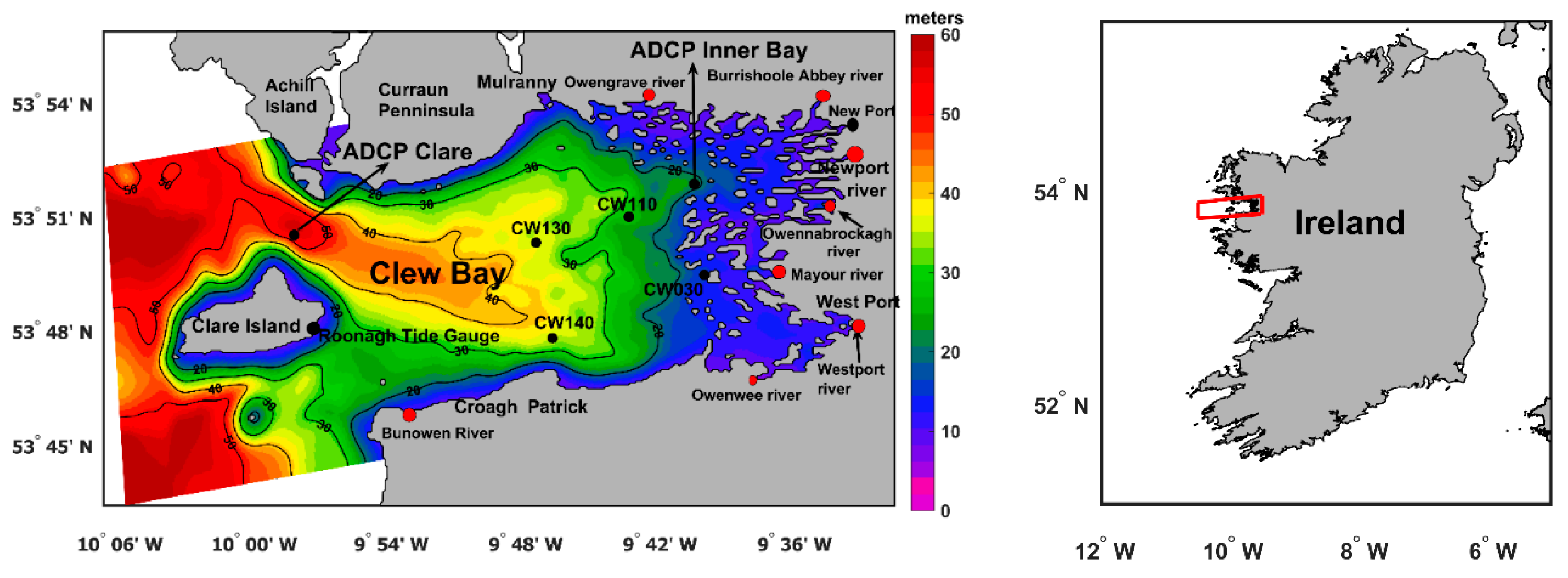
Figure 2.
Temporal comparison between the Clew Bay model (in continuous red lines) and ADCPs (in continuous blue lines) bottom temperature in [oC] for the period from 25th July until 20th December 2017 where, (a) Inner Bay ADCP located at 9.67°W, 53.86°N with water depth of 15 meters (b) Clare Island ADCP located at 9.97°W, 53.84°N with water depth of 40 meters.
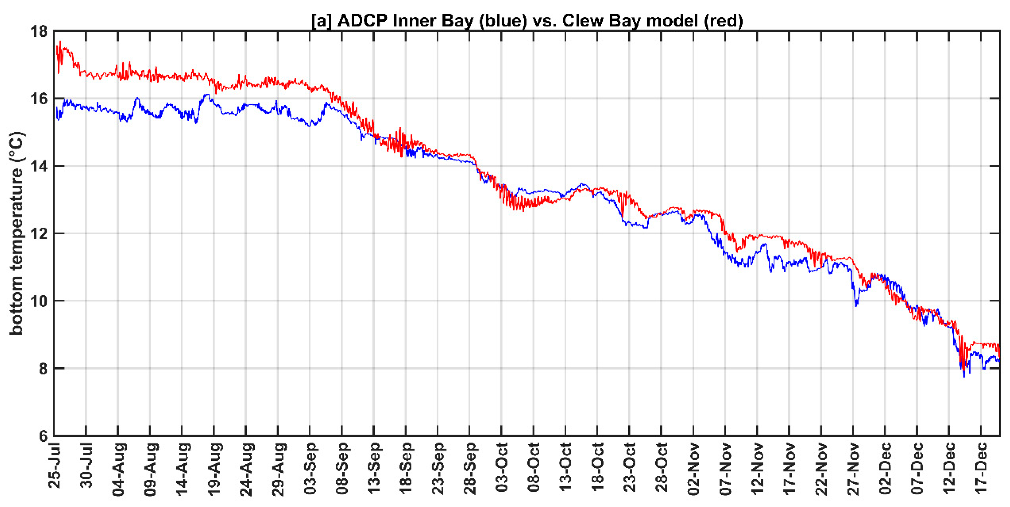
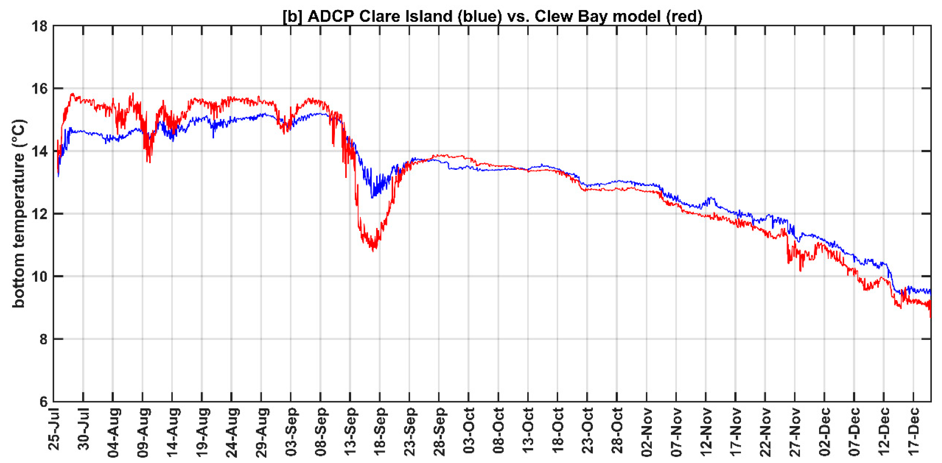
Figure 3.
Taylor diagram assessing the bottom temperature representation, in terms of correlation, STD in [oC] and RMSD in [oC] by the Clew Bay model and ADCPs temperature in [oC] for the period from 25th July until 20th December 2017 on 12 minutes frequency where the observations (black solid circle) where,(a) Inner Bay ADCP located at 9.67°W, 53.86°N with water depth of 15 meters (red solid circle), and (b) Clare Island ADCP located at 9.97°W, 53.84°N with water depth of 40 meters (red solid circle).
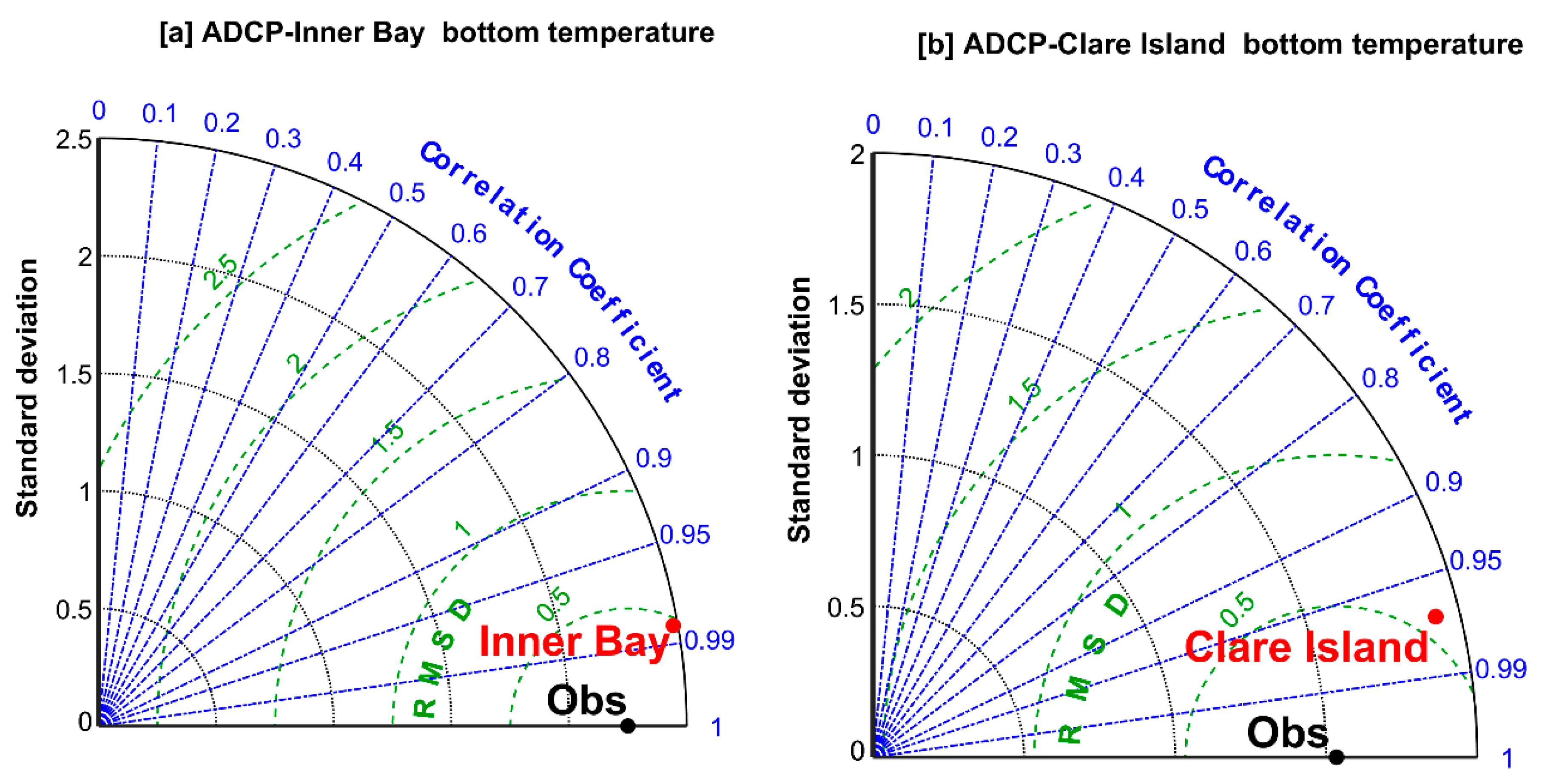
Figure 4.
Taylor diagrams assessing the barotropic velocity components representation, in terms of correlation, STD in [m/s] and RMSD in [m/s], by the Clew Bay model and ADCPs barotropic velocity components in [m/s] for the period from 25th July until 20th December 2017 on 12 minutes frequency where the observations (ADCPs black solid circle) where (a,b) East barotropic velocity component (u) (c,d) North barotropic velocity component (v). For Clare Island ADCP located at 9.97°W, 53.84°N with water depth of 40 meters (red solid circle) and Inner Bay ADCP located at 9.67°W, 53.86°N with water depth of 15 meters (red solid circle).
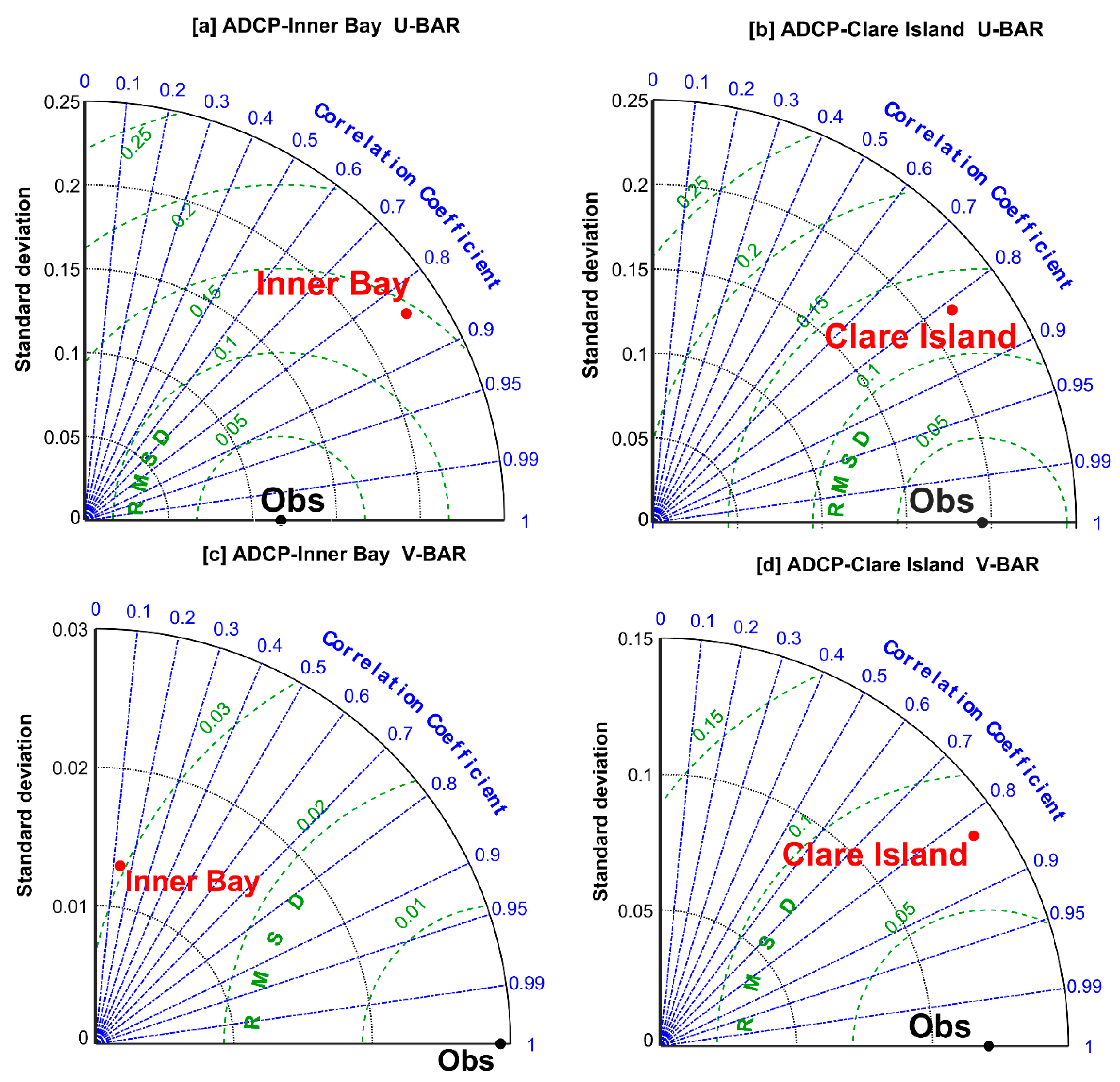
Figure 5.
Vertical profiles of modelled (continuous red lines) temperature, salinity, and density and observations (continuous blue lines) for different EPA stations on 20, September 2017. The EPA stations are, from top to bottom, (a) CW030, (b) CW110, (c) CW130 and (d) CW140. The right panel maps for the EPA stations location.
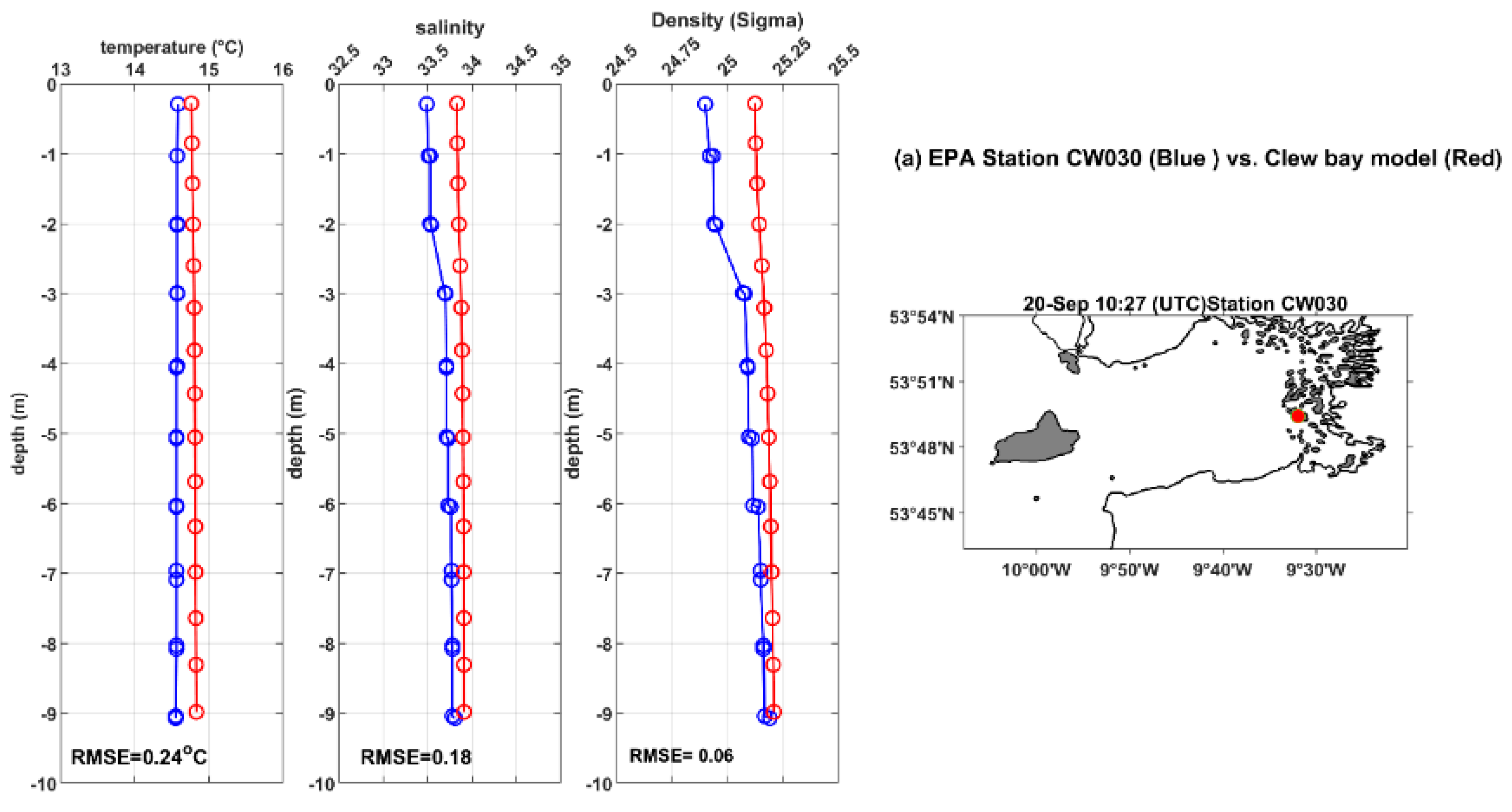
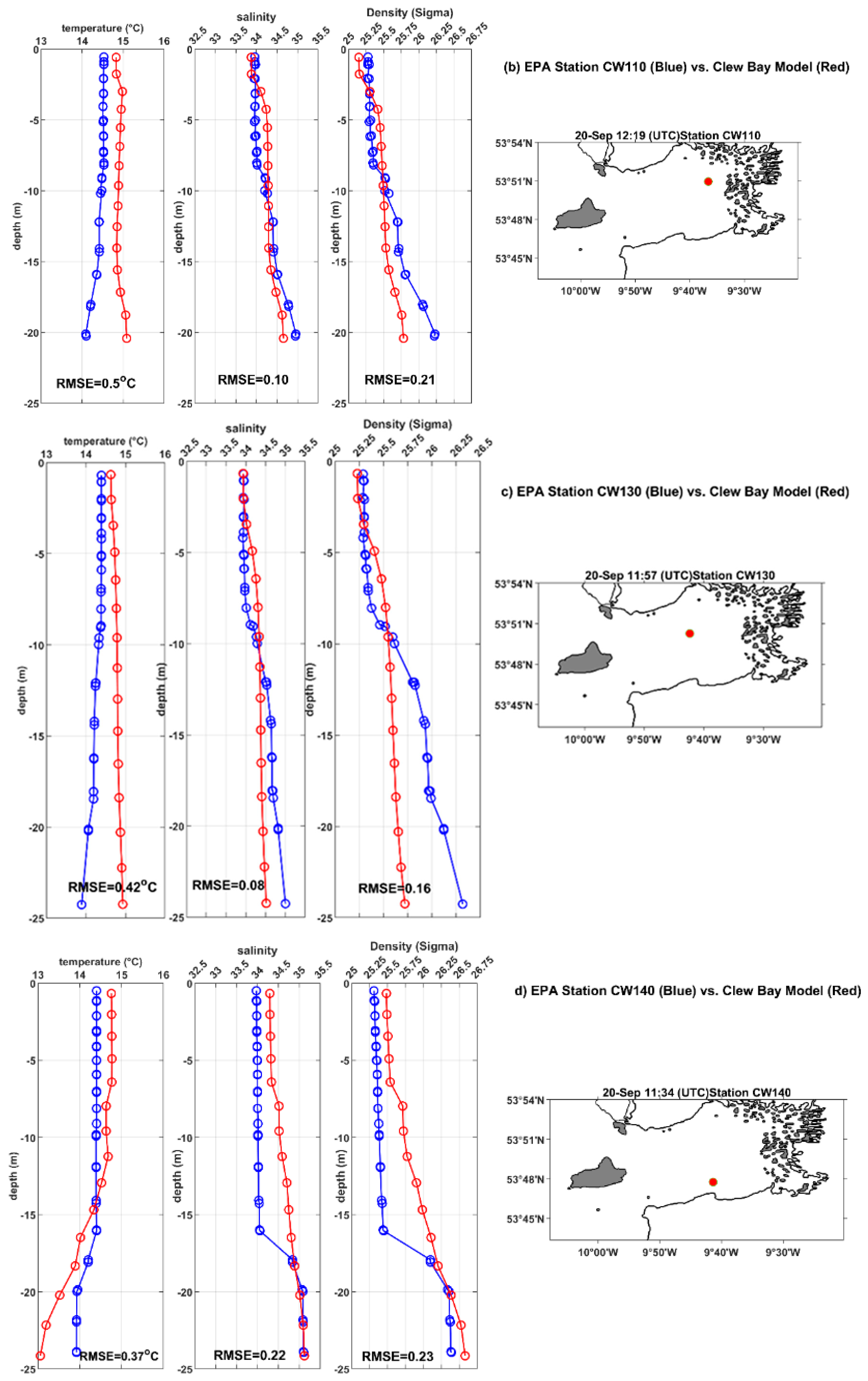
Figure 6.
Taylor diagram assessing the Sea Surface Height (SSH) representation, in terms of correlation, STD and RMSD in meters, made by Clew Bay Model and Roonagh Tide Gauge Station Sea Surface Height (SSH) [meters]. The diagram is based on the period from 14th of August 2017 until 2nd of January 2018 on 6 minutes frequency where the observations (Tide Gauge black solid circle) and Model (Red solid circle).
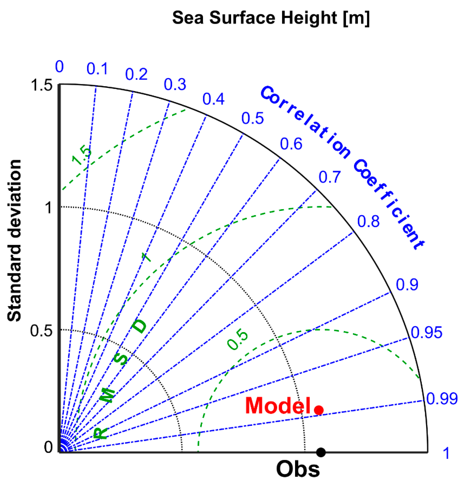
Figure 7.
Monthly averaged barotropic velocity [m/sec] fields (speed and direction denoted by arrows). (a) January (b) July.
Figure 7.
Monthly averaged barotropic velocity [m/sec] fields (speed and direction denoted by arrows). (a) January (b) July.
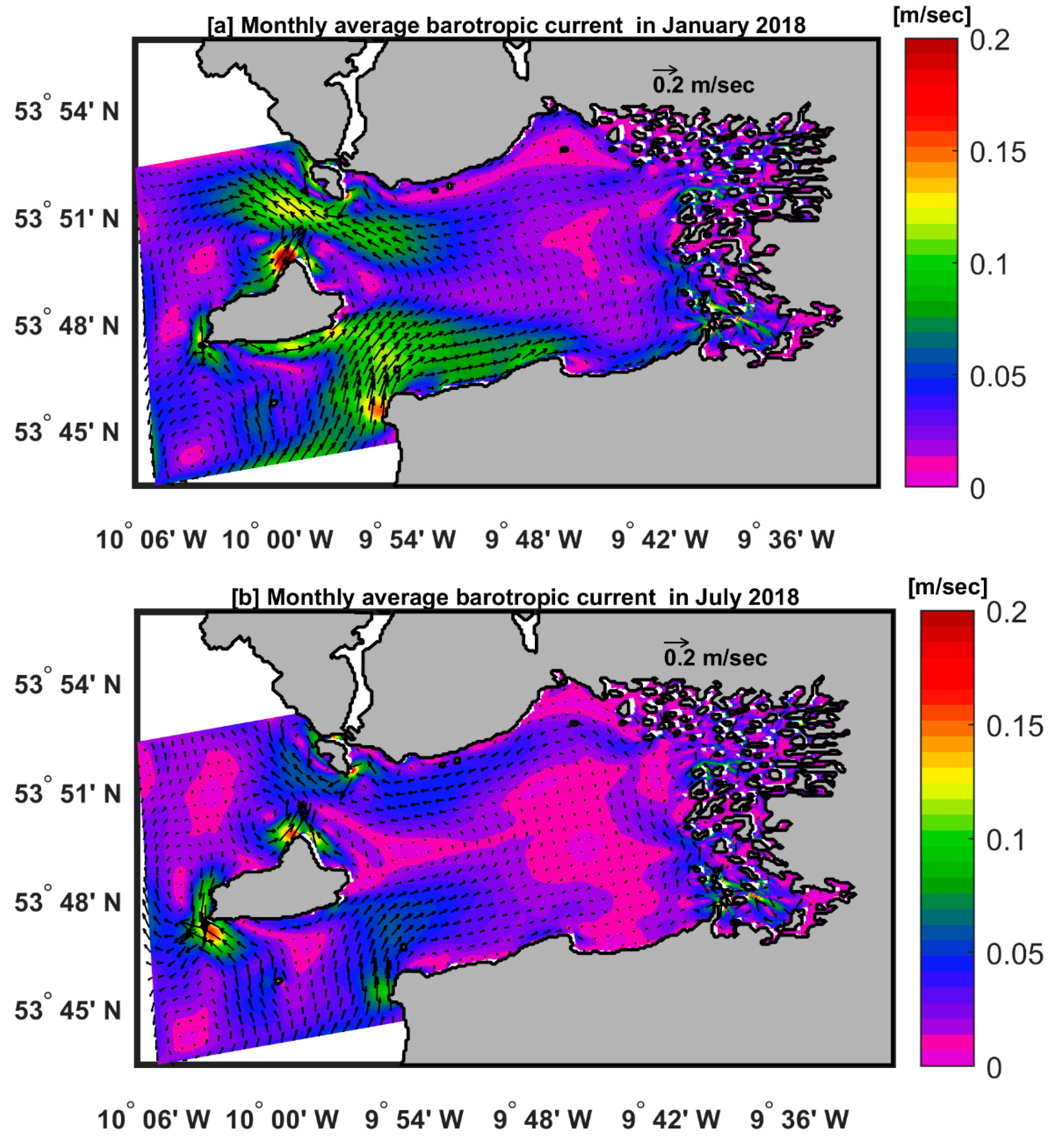
Figure 8.
Residual barotropic velocity [m.s-1] fields (speed and direction denoted by vectors or arrows) and (a)spring tide averaged over 10th of September 2018, (b) neap tide averaged over 2nd of October 2018.
Figure 8.
Residual barotropic velocity [m.s-1] fields (speed and direction denoted by vectors or arrows) and (a)spring tide averaged over 10th of September 2018, (b) neap tide averaged over 2nd of October 2018.
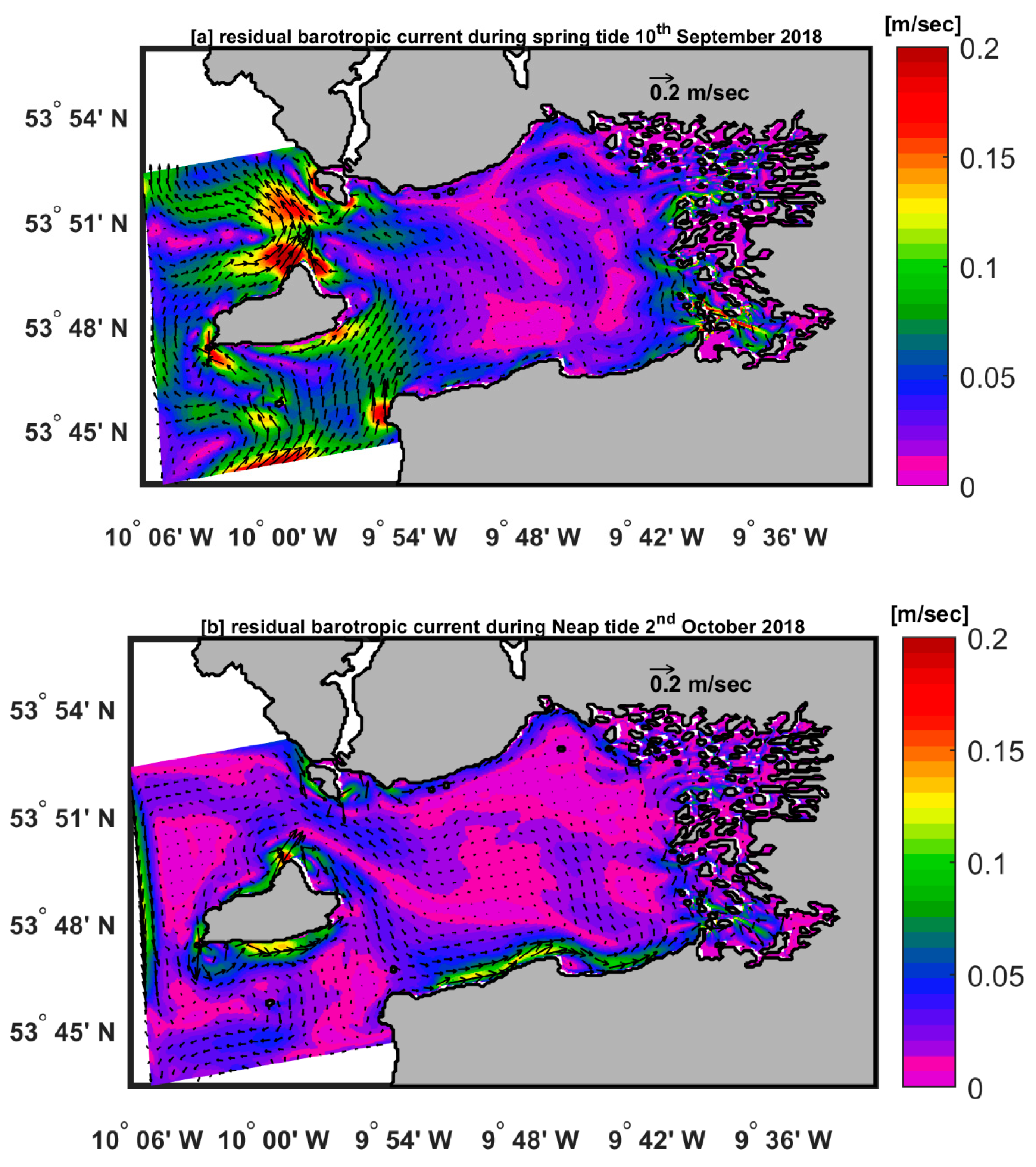
Figure 9.
(a) The monthly average values of net flow in [m3/s] over the cross-section shown on the map. (b) The monthly average values of wind speed [m/s] over the cross section shown in the map (c).
Figure 9.
(a) The monthly average values of net flow in [m3/s] over the cross-section shown on the map. (b) The monthly average values of wind speed [m/s] over the cross section shown in the map (c).
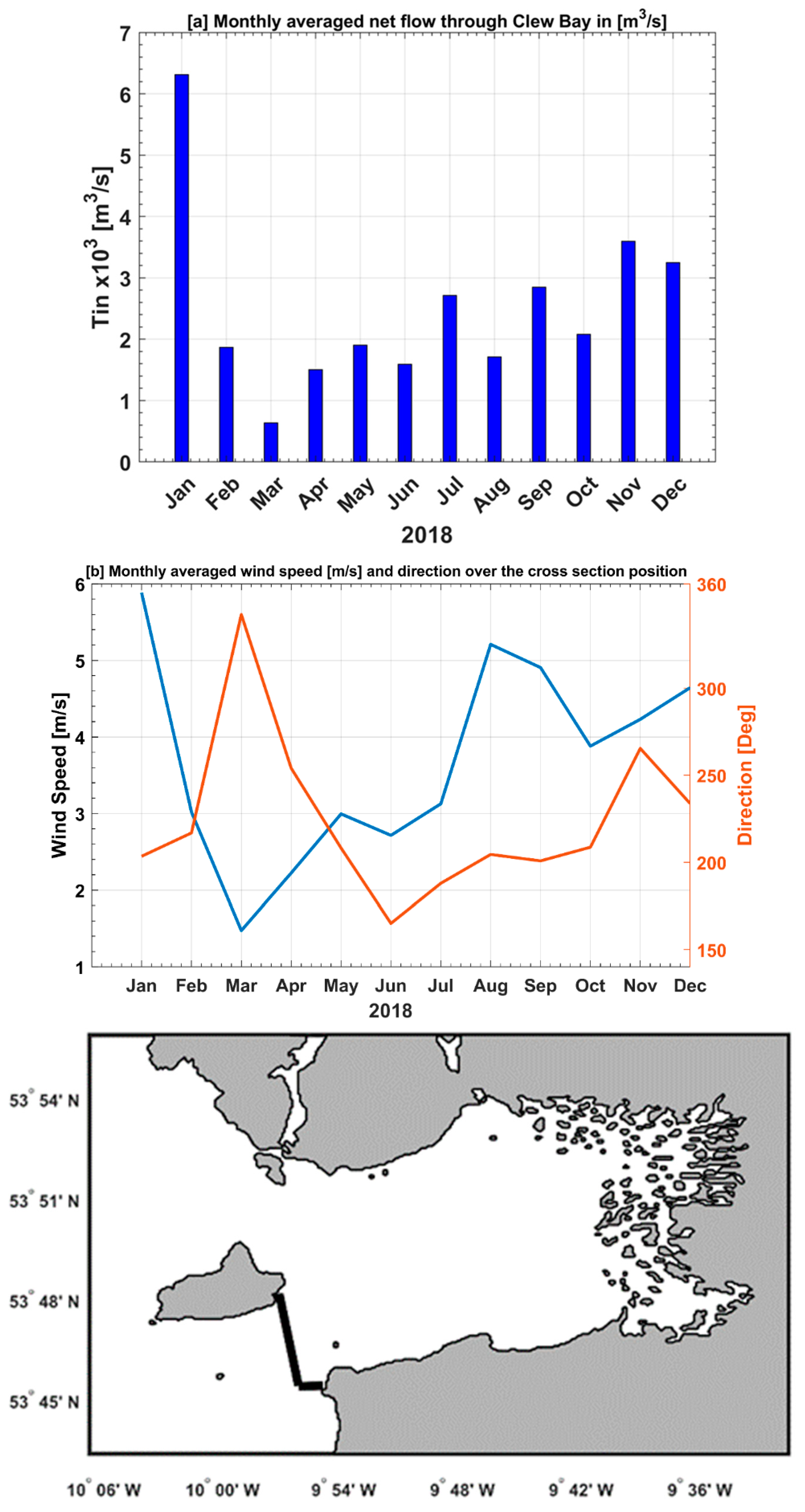

Table 1.
Mean annual freshwater discharge values [m3/s], in the Clew Bay model.
| Region | River Name | Mean Annual Discharge [m3/s] |
|---|---|---|
| Clew Bay | Owenwee | 7.61 |
| Newport | 5.54 | |
| Bunowen | 3.17 | |
| Owengrave | 2.49 | |
| Mayour | 1.99 | |
| Westport | 1.64 | |
| Owennabrockagh | 1.98 | |
| Burrishoole Abbey | 4.98 |
Table 2.
The EPA station locations for temperature and salinity profiles in latitude and longitude (in degrees) sampled on 20th September 2017.
Table 2.
The EPA station locations for temperature and salinity profiles in latitude and longitude (in degrees) sampled on 20th September 2017.
| Station Name | Latitude °N | Longitude °W |
|---|---|---|
| CW030 | 53.82 | 9.66 |
| CW110 | 53.85 | 9.72 |
| CW130 | 53.84 | 9.79 |
| CW140 | 53.80 | 9.78 |
Table 3.
The amplitudes in meters and phases in degrees for six of the principal tidal constituents calculated, for the measured and modelled data with the differences (Model- Tide Gauge) between them for the period from 14th August 2017 until 2nd January 2018.
Table 3.
The amplitudes in meters and phases in degrees for six of the principal tidal constituents calculated, for the measured and modelled data with the differences (Model- Tide Gauge) between them for the period from 14th August 2017 until 2nd January 2018.
| Tidal (Main) Components | Model Amplitude |
T.G Amplitude | Difference | Model (Phase Angle) |
T.G (Phase Angle) |
Difference |
|---|---|---|---|---|---|---|
| M2 | 1.360 | 1.310 | +0.050 | 180.22 | 180.65 | - 0.43 |
| S2 | 0.509 | 0.508 | +0.001 | 212.62 | 210.28 | +2.34 |
| N2 | 0.278 | 0.263 | +0.015 | 158.72 | 161.72 | -3.00 |
| K1 | 0.136 | 0.135 | +0.001 | 105.27 | 96.08 | + 9.19 |
| O1 | 0.073 | 0.078 | -0.005 | 329.97 | 333.08 | -3.11 |
| Q1 | 0.011 | 0.011 | 0.000 | 299.23 | 301.01 | -1.78 |
Disclaimer/Publisher’s Note: The statements, opinions and data contained in all publications are solely those of the individual author(s) and contributor(s) and not of MDPI and/or the editor(s). MDPI and/or the editor(s) disclaim responsibility for any injury to people or property resulting from any ideas, methods, instructions or products referred to in the content. |
© 2023 by the authors. Licensee MDPI, Basel, Switzerland. This article is an open access article distributed under the terms and conditions of the Creative Commons Attribution (CC BY) license (http://creativecommons.org/licenses/by/4.0/).
Copyright: This open access article is published under a Creative Commons CC BY 4.0 license, which permit the free download, distribution, and reuse, provided that the author and preprint are cited in any reuse.


