You are currently viewing a beta version of our website. If you spot anything unusual, kindly let us know.

Preprint

Article

Benchmarking Gradient Based Optimizers’ Sensitivity to Learning Rate

Altmetrics

Downloads

193

Views

Comments

Rehan Guha^*

This version is not peer-reviewed

This preprints belongs to the Topic

Machine and Deep Learning

Abstract

Initial choice of Learning Rate is a key part of gradient based methods and has a great effect on the performance of the Deep Learning Model.This paper studies the behavior of multiple gradient based optimization algorithm which are commonly used in Deep Learning and compare their performance on various learning rate. As observed popular choice of optimization algorithms are highly sensitive to various choice of learning rates. Our goal is to find which optimizer has an edge over others for a specific setting. We look at two datasets namely MNIST and CIFAR10 for benchmarking. The results are quite surprising, and it will help us to choose a learning rate more efficiently.

Keywords:

Subject: Computer Science and Mathematics - Artificial Intelligence and Machine Learning

1. Introduction

Stochastic gradient-based optimization is of core practical importance in many fields of science and engineering. Many problems in these fields can be cast as the optimization of some scalar parameterized objective function requiring maximization or minimization with respect to its parameters. If the function is differentiable w.r.t. its parameters, gradient descent is a relatively efficient optimization method, since the computation of first-order partial derivatives w.r.t. all the parameters is of the same computational complexity as just evaluating the function. Often, objective functions are stochastic.

Learning Rate plays a key role for all gradient based optimizers and here we will experiment on various dataset, using multiple gradient based optimizers. We will propose and try to show that all optimizers are extremely dependent on the type of the data, learning rate and different type of deep learning models. This will give us an idea on how to efficiently choose an optimizer depending on the data and, is the optimizer sensitive to different values of learning rate.

2. Background & Related Work

When it comes to the selection of Learning Rate it is popularly said that the range of values considered for learning rate is less than (1.0) and greater than (

10^{- 6}

) [1]. The choice of the value for the learning rate can be fairly critical, since if it is too small the reduction in error will be very slow, while, if it is too large, divergent oscillations can result [2]. Generally, A default value of 0.01 typically works for standard multi-layer neural networks, but it would be foolish to rely exclusively on this default value [1].

One of the most popular ways to fix the value of learning rate is using grid search. Typically, a grid search involves picking values approximately on a logarithmic scale, e.g., a learning rate taken within the set

(. 1, . 01, 10^{- 3}, 10^{- 4}, 10^{- 5}

) [3].

Another technique we can use is to use adaptive learning rate using a momentum. The method of momentum is designed to accelerate learning, especially in the face of high curvature, small but consistent gradients, or noisy gradients. The momentum algorithm introduces a variable

' v'

that plays the role of velocity — it is the direction and speed at which the parameters move through parameter space. The velocity is set to an exponentially decaying average of the negative gradient. [3]

In this paper we will keep the learning rate constant as per their respective paper or the tensorflow repo default throughout the training process, and just observe the change in behavior with respect to training accuracy/loss and test accuracy/loss. We will use some adaptive learning rate optimizers as well, to see their performance over a constant one.

3. Experiment Setting

The entire experiment is performed on multiple datasets and the observation is quite interesting as some optimizer’s performance is stable and better performing than the rest. We have used popular dataset to benchmark the results. Datasets which we have used for this experiment are MNIST, CIFAR10. The metrics which we will use to compare all the algorithms are Training Accuracy, Test Accuracy and Training Loss and Test Loss.

Now, for the MNIST data we have used the below simple neural network:

We have also tested using the below Convolutional Neural Network(CNN) with the CIFAR-10 dataset.

We have iterated over

[0.001, 0.003, 0.01, 0.03, 0.1]

different range of values of Learning Rate. Along with this we swept over different values of epochs

[50, 100, 150, 200]

, all the details are available on the "Supplementary Materials" section. Along with this we iterated over all values of learning rate from 0.01 to 0.1 with step size of 0.01, epoch=200 and captured all the performance.

3.1. Optimizer

In this section we have discussed all the optimizers which we have used in this paper. Here, I have standardized all the equations and the greek letters, so that we can compare them easily, hence the equations might be different from the papers.

Some notations used for the following equations:

t -Time step
$w_{t}$ -Weight/parameter at the given time step
$α$ - Learning rate
$\frac{\partial L}{\partial w_{t}}$ -Gradient of the Loss Function (L) to minimize w.r.t. w

3.1.1. SGD

Stochastic gradient descent (SGD) is one of the earliest and popular approach for an optimization algorithm as it performs a parameter update for each training example.

w_{t + 1} = w_{t} - α \frac{\partial L}{\partial w_{t}}

3.1.2. Adagrad

Adaptive gradient, or Adagrad [4] is an optimizer with parameter-specific learning rates, which are adapted relative to how frequently a parameter gets updated during training. The more updates a parameter receives, the smaller the updates. Note that the gradient component remains unchanged like in SGD.

w_{t + 1} = w_{t} - \frac{α}{\sqrt{v_{t} + ϵ}} \cdot \frac{\partial L}{\partial w_{t}}

where,

v_{t} = v_{t - 1} + {[\frac{\partial L}{\partial w_{t}}]}^{2}

And by default v is initialized to 0.

We can see in the equation that an

ϵ

term is added with

v_{t}

which is called the fuzz factor by Keras, and it is used to avoid division by zero error.

The default values (from TensorFlow):

α = 0.01

and

ϵ = 10^{- 7}

3.1.3. RMSProp

Root mean square prop or RMSprop [5] is an unpublished, adaptive learning rate method proposed by Geoff Hinton in Lecture 6e of his Coursera.

RMSProp is a stochastic technique for mini-batch learning which tries to improve Adagrad. RMSprop deals with the above issue by using an exponential moving average of squared gradients to normalize the gradient. This normalization balances the step size (momentum), decreasing the step for large gradients to avoid exploding, and increasing the step for small gradients to avoid vanishing. RMSprop uses an adaptive learning rate instead of treating the learning rate as a hyperparameter. This means that the learning rate changes over time.

w_{t + 1} = w_{t} - \frac{α}{\sqrt{v_{t} + ϵ}} \cdot \frac{\partial L}{\partial w_{t}}

where,

v_{t} = β v_{t - 1} + (1 - β) {[\frac{\partial L}{\partial w_{t}}]}^{2}

And v is initialized as 0.

The default values (from TensorFlow):

α = 0.001

β = 0.9

(recommended by the authors of the paper) and

ϵ = 10^{- 6}

3.1.4. Adadelta

Adadelta [5] optimization is a stochastic gradient descent method that is based on adaptive learning rate per dimension to address two drawbacks:

The continual decay of learning rates throughout training
The need for a manually selected global learning rate

Adadelta is a more robust extension of Adagrad that adapts learning rates based on a moving window of gradient updates, instead of accumulating all past gradients. This way, Adadelta continues learning even when many updates have been done.

The difference between Adadelta and RMSprop is that Adadelta removes the use of the learning rate parameter completely by replacing it with D, the exponential moving average of squared deltas.

w_{t + 1} = w_{t} - \frac{\sqrt{D_{t - 1} + ϵ}}{\sqrt{v_{t} + ϵ}} \cdot \frac{\partial L}{\partial w_{t}}

where,

\begin{matrix} D_{t} & = β D_{t - 1} + (1 - β) {[Δ w_{t}]}^{2} \\ v_{t} & = β v_{t - 1} + (1 - β) {[\frac{\partial L}{\partial w_{t}}]}^{2} \\ Δ w_{t} & = w_{t} - w_{t - 1} \end{matrix}

Compared to Adagrad, in the original version of Adadelta you don’t have to set an initial learning rate. In this version, initial learning rate can be set, as in most other TensorFlow (Keras) optimizers.

The default values (from TensorFlow):

β = 0.95

and

ϵ = 10^{- 6}

3.1.5. Adam

Adaptive moment estimation, or Adam [6] optimization is a stochastic gradient descent method that is based on adaptive estimation of first-order and second-order moments. According to Kingma et al. [6], 2014, the method is "computationally efficient, has little memory requirement, invariant to diagonal rescaling of gradients, and is well suited for problems that are large in terms of data/parameters".

w_{t + 1} = w_{t} - \frac{α}{\sqrt{{\hat{v}}_{t}} + ϵ} \cdot {\hat{m}}_{t}

where,

\begin{matrix} {\hat{m}}_{t} & = \frac{m_{t}}{1 - β_{1}^{t}} \\ {\hat{v}}_{t} & = \frac{v_{t}}{1 - β_{2}^{t}} \end{matrix}

{\hat{m}}_{t}

and

{\hat{v}}_{t}

are the bias correction, and

\begin{matrix} m_{t} & = β_{1} m_{t - 1} + (1 - β_{1}) \frac{\partial L}{\partial w_{t}} \\ v_{t} & = β_{2} v_{t - 1} + (1 - β_{2}) {[\frac{\partial L}{\partial w_{t}}]}^{2} \end{matrix}

With m and v initialized to 0.

As per the authors of the paper the default values are:

α = 0.001

β_{1} = 0.9

β_{2} = 0.999

and

ϵ = 10^{- 8}

3.1.6. Adamax

AdaMax [6] is an adaptation of the Adam optimizer by the same authors using infinity norms (hence ‘max’). Default parameters follow those provided in the paper. Adamax is sometimes superior to adam, specially in models with embeddings.

w_{t + 1} = w_{t} - \frac{α}{v_{t}} \cdot {\hat{m}}_{t}

where,

{\hat{m}}_{t} = \frac{m_{t}}{1 - β_{1}^{t}}

{\hat{m}}_{t}

is the bias correction for m, and

\begin{matrix} m_{t} & = β_{1} m_{t - 1} + (1 - β_{1}) \frac{\partial L}{\partial w_{t}} \\ v_{t} & = max (β_{2} v_{t - 1}, |\frac{\partial L}{\partial w_{t}}|) \end{matrix}

With m and v initialized to 0.

As per the authors of the paper the default values are:

α = 0.002

β_{1} = 0.9

and

β_{2} = 0.999

3.1.7. Nadam

Nadam [7] is an acronym for Nesterov and Adam optimizer. Much like Adam is essentially RMSprop with momentum, Nadam is Adam with Nesterov momentum.

Adam optimizer can also be written as:

w_{t + 1} = w_{t} - \frac{α}{\sqrt{{\hat{v}}_{t}} + ϵ} (β_{1} {\hat{m}}_{t - 1} + \frac{1 - β_{1}}{1 - β_{1}^{t}} \cdot \frac{\partial L}{\partial w_{t}})

Nadam uses Nesterov to update the gradient one step ahead by replacing the previous

{\hat{m}}_{t - 1}

in the above equation to the current

{\hat{m}}_{t}

w_{t + 1} = w_{t} - \frac{α}{\sqrt{{\hat{v}}_{t}} + ϵ} (β_{1} {\hat{m}}_{t} + \frac{1 - β_{1}}{1 - β_{1}^{t}} \cdot \frac{\partial L}{\partial w_{t}})

where, Keras t and

{\hat{v}}_{t}

are the bias correction, and

\begin{matrix} m_{t} & = β_{1} m_{t - 1} + (1 - β_{1}) \frac{\partial L}{\partial w_{t}} \\ v_{t} & = β_{2} v_{t - 1} + (1 - β_{2}) {[\frac{\partial L}{\partial w_{t}}]}^{2} \end{matrix}

With m and v initialized to 0.

The default values (from TensorFlow):

α = 0.002

β_{1} = 0.9

β_{2} = 0.999

and

ϵ = 10^{- 7}

3.2. Datasets

3.2.1. MNIST

The MNIST database of handwritten digits, available from this page, has a training set of 60,000 examples, and a test set of 10,000 examples. It is a subset of a larger set available from NIST. The digits have been size-normalized and centered in a fixed-size image.

3.2.2. CIFAR10

The CIFAR-10 dataset consists of 60000 32x32 color images in 10 classes, with 6000 images per class. There are 50000 training images and 10000 test images.

The dataset is divided into five training batches and one test batch, each with 10000 images. The test batch contains exactly 1000 randomly-selected images from each class. The training batches contain the remaining images in random order, but some training batches may contain more images from one class than another. Between them, the training batches contain exactly 5000 images from each class.

4. Results and Discussion

We can divide the tested optimization algorithms in few groups w.r.t. Learning Rate sensitivity:

Algorithms which are heavily impacted by different learning rates and change in the output performance is significant, in terms of accuracy and loss for both training and testing data.
Some optimization algorithms have low to none impact on the output, if the model is executed for higher number of epochs.
There are some algorithms which are tough to categorize into the above two groups as the behavior is not constant over all datasets, entire range of epochs, and different values of LR.

4.1. MNIST

4.1.1. Visualization

In MNIST dataset we will split the optimizers into different groups, one being the where the optimizers are not sensitive or less sensitive towards different values of learning rates and another category is where the optimizers are sensitive or highly sensitive towards different values of learning rate.

Let us start visualizing the first category where the optimizers are less to no sensitive towards different values of learning rates.

Figure 1. Accuracy of non-sensitive optimizers over 100 different values of Learning Rate (epoch=200)

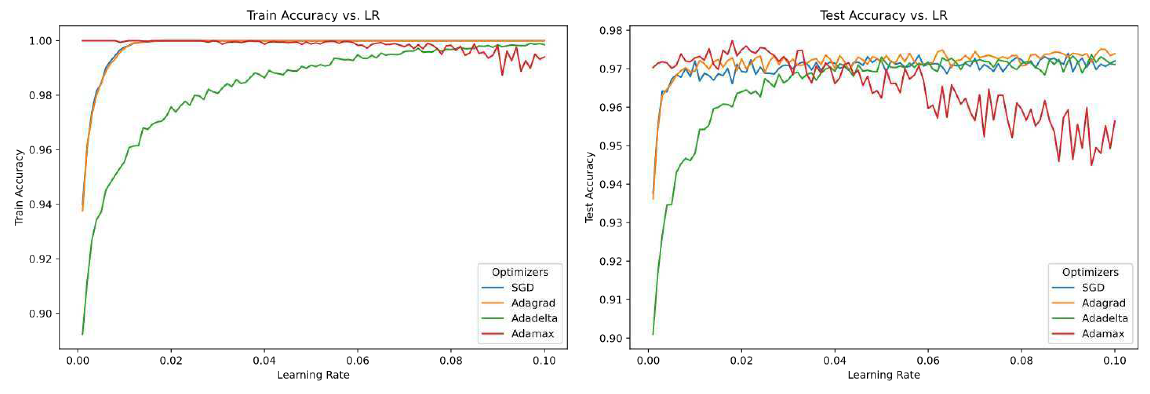
From the above figure we can clearly see that SGD, Adagrad, Adadelta performed best over both training data and test data. But, Adamax performs similarly over a range of learning rate and the accuracy converges for the training dataset and for the test dataset the accuracy decreases compared to rest of the optimizers. Adamax clearly performs better for lower values of learning rate and Adadelta performs better for higher values of learning rate.

Now we will see another group of optimizers which are sensitive towards different values of learning rate.

Figure 2. Accuracy of sensitive optimizers over 100 different values of Learning Rate (epoch=200)

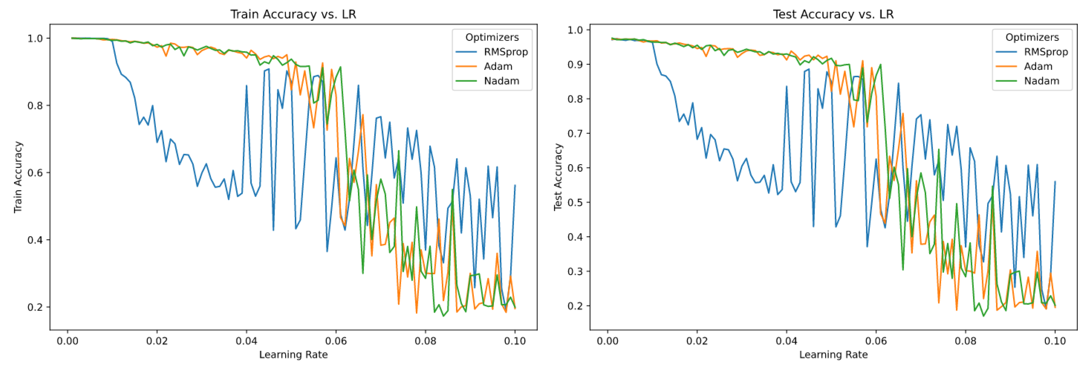
Above figure shows the optimizers which are sensitive to different values of optimizers. RMSprop shows the sensitivity from the lower value of learning rate and rest of optimizers Adam and Nadam starts to show the sensitivity from somewhere from middle range values of learning rate.

4.1.2. Optimizers

In this subsection we will individually analyze each optimizer using the above figures and some additional figures from the supplementary material on page number Table 1.

SDG

Varied learning rate over different epochs has no effect over training accuracy and validation accuracy.
RMSProp

In the case of RMSProp, learning rate $\in {0.01, 0.003, 0.001}$ for the training and validation accuracy converges after a few iterations.

But, for the higher value of the learning rate $\in {0.03, 0.1}$ the accuracy tends to decrease over time, and it diverges.

These pattern seems to be consistent for different epochs and RMSProp seem to be highly LR sensitive for MNIST dataset.
ADAM

ADAM is similar to RMSProp, and it is only sensitive ti learning rate for higher values of LR.

For LR $\in {0.1}$ , the accuracy does not converge to the same point.

For rest of the LR it converges to a same point with higher accuracy for both training and validation data.
Adagrad

Adagrad is one of the optimizers which is completely insensitive towards different values of learning rate over a range of epochs.

For all the training and validation data it performs similarly and converges towards a same point with higher accuracy.
Adadelta

Adadelta is from the list of optimizers which is not sensitive to learning rates. But, all the accuracy of different LR does not converge at a same point. The deviation is quite high compared to the other optimizers (which are not sensitive towards different value of LRs).

Higher value of LR has more accuracy compared to lower value of LR.

For this unique property I would tag this optimizer to a different group where the change of LR has moderate effect over training and validation accuracy and higher value of LR performs better compared to a lower version of the LR or vice-versa.
Adamax

This optimizer has no effect on the accuracy with different learning rate.

But, it follows a similar pattern compared to Adadelta, where the higher values of LR is a bit diverged compared to other value of LR for all epochs.
Nadam

Nadam has a great result for lower value of LR’s. But for higher value of LR’s the performance decreases and diverges.

So, Nadam is sensitive to higher value of learning rates.

4.2. CIFAR-10

4.2.1. Visualization

Figure 3. Accuracy of non-sensitive optimizers over 100 different values of Learning Rate (epoch=200).

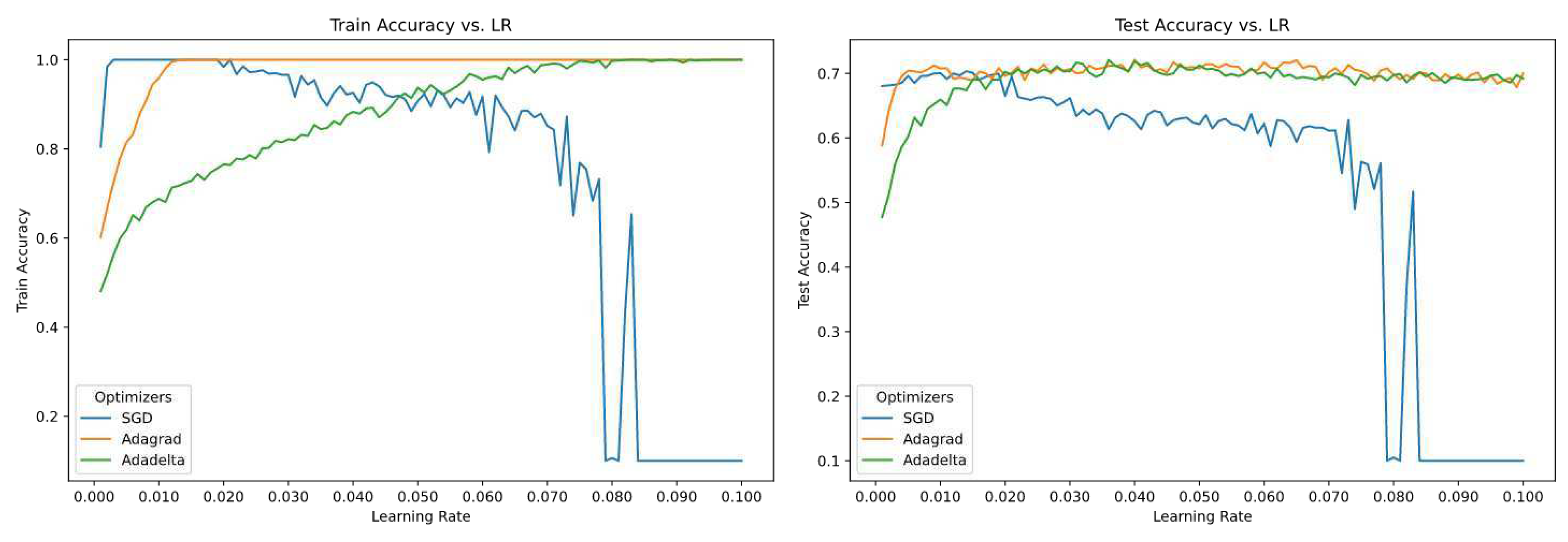
From the above figure we can clearly see that Adagrad, Adadelta performed best over both training data and test data, and they are the least sensitive towards But, SGD performs similarly over a range of learning rate and the accuracy converges for the training dataset and for the test dataset the accuracy decreases compared to rest of the optimizers. SGD clearly performs better for lower values of learning rate and Adadelta performs better for higher values of learning rate.

Now we will see another group of optimizers which are sensitive towards different values of learning rate.

Figure 4. Accuracy of sensitive optimizers over 100 different values of Learning Rate (epoch=200)

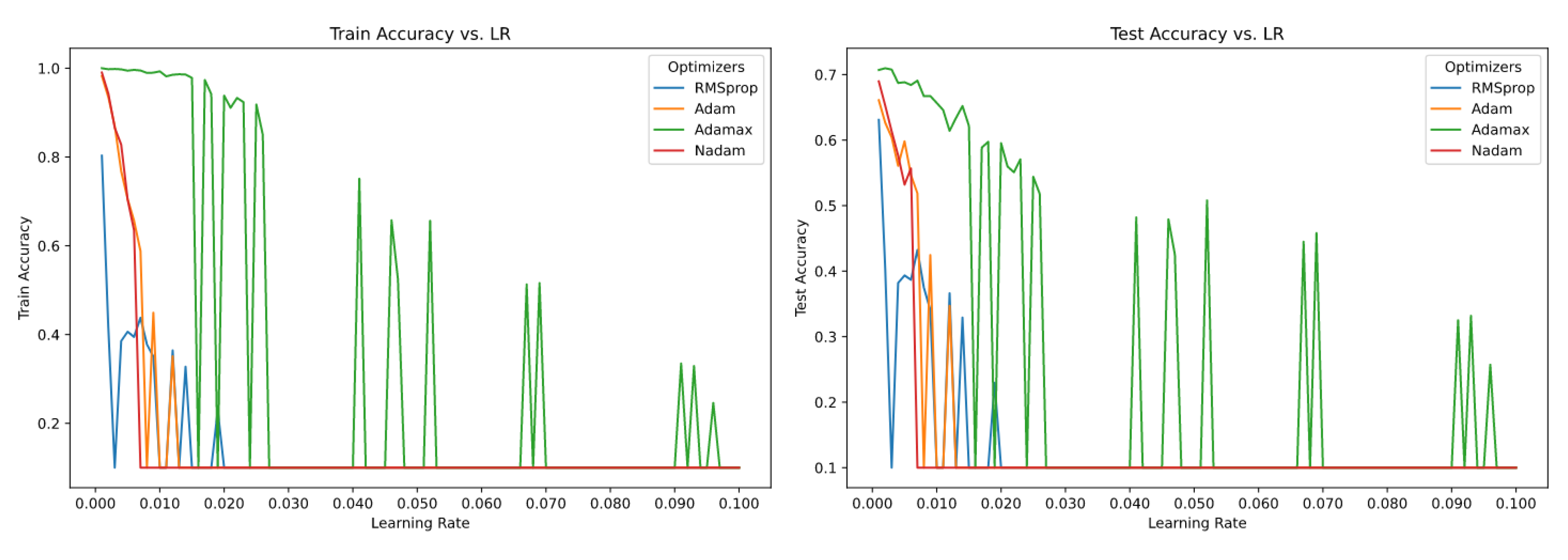
Above figure shows the optimizers which are sensitive to different values of optimizers. Adamax shows the sensitivity for the higher values of learning rate and rest of optimizers RMSProp, Adam and Nadam starts to show the sensitivity from somewhere from middle range values of learning rate.

4.2.2. Optimizers

In this subsection we will individually analyze each optimizer using the above figures and some additional figures from the supplementary material on page number Table 2.

SDG

SGD for CIFAR10 dataset with different learning rate has a moderate effect on the accuracy.

Lower value of learning rate converges to similar accuracy at higher epochs. Then there is a sudden drop in accuracy from the epoch value around 130.
RMSProp

RMSProp is highly sensitive to different learning rate across all epochs.

Performance of the model with higher value of learning rate has the least accuracy and lower value of learning yields a better performance.
Adam

Adam performs similar to RMSProp. The model with lower value of learning rate performs better w.r.t. accuracy compared to the model with higher values of learning rate.

Here, we see for the models with higher value of learning rate does not converge to a similar value of accuracy for higher value of epochs.
Adagrad

This optimizer is highly sensitive to models with different values of learning rate.

Surprisingly, models with higher value of learning rate has a better accuracy compared to the models with lower value of learning rate.

With respect to convergence none of the model’s accuracy with different learning rate converged to a similar accuracy over all the given epochs.
Adadelta

The model with higher value of learning rate has a better performance compared to the models with lower values of learning rate.

The optimizer is sensitive towards different values of learning rate over multiple epoch values.

The optimizer is highly sensitive towards different values of learning rate and at the same time the divergence is constant.
Adamax

The optimizer’s performance is best when the value of learning rate of the model is small. Higher the value of learning rate for the model lower the accuracy, and it tends to diverge as well.

We can clearly say that the model with lower values of learning rate shows no sensitivity over multiple epochs.
Nadam

This optimizer performs similar to Adamax

5. Conclusion

This paper shows us that we should be careful with choosing the right optimizer for the given problem.

I started with a notion that all optimizers’ performance is similar when we train for higher number of epochs. We can clearly see from the above experiment that the optimizer has a huge role for the performance of the model. It is evident from that Adagrad and Adadelta optimizers are the best performing algorithms for both of the datasets over the range of all the learning rates. The stability in the performance is higher compared to rest of the algorithms tested. Some algorithms like SGD and Adamax does perform well for one of the datasets only, and they are quite unstable in terms of per the test accuracy of the model when the learning rate is close to

0.1

. Some optimizers like RMSProp, Adam, Nadam perform consistently bad compared to rest of the optimizers. They tend to have a bad performance overall throughout the range of the entire We can conclude that choosing a right algorithm for optimizer is critical in terms of getting the right accuracy for the model training, and it can drastically reduce the amount of computational budget. It is also advised to test with more than one best performing optimizers to confirm which algorithm performs the best for the setting.

6. Future Work

With the above experiment we can clearly see that the optimizers plays a huge role in the performance of the model. It will be great if the optimizer’s performance can be quantified for various set of data. It will make choosing the right optimizer faster. As the data is constant the all the different optimizers, but the performance varies a lot, so it will be great to know the factors which cause this kind of behavior for the optimizers. Some optimizers from the tested on.

Supplementary Materials

The following supporting information can be downloaded at the website of this paper posted on Preprints.org.

Acknowledgments

Conflicts of Interest

References

Bengio, Y. Practical recommendations for gradient-based training of deep architectures. arXiv:1206.5533 [cs], 2012; arXiv:1206.5533. [Google Scholar] [CrossRef]
Bishop, C.M. Neural Networks for Pattern Recognition. p. 251.
Ian Goodfellow. Deep Learning | The MIT Press. Publisher: The MIT Press.
Duchi, J.; Hazan, E.; Singer, Y. Adaptive Subgradient Methods for Online Learning and Stochastic Optimization. p. 39.
Zeiler, M.D. ADADELTA: An Adaptive Learning Rate Method. arXiv:1212.5701 [cs], 2012; arXiv:1212.5701. [Google Scholar] [CrossRef]
Kingma, D.P.; Ba, J. Adam: A Method for Stochastic Optimization. arXiv:1412.6980 [cs], 2017; arXiv:1412.6980. [Google Scholar] [CrossRef]
Dozat, T. Incorporating Nesterov Momentum into Adam. p. 6.

Table 1. Model setting for MNIST Dataset.

Model: "sequential"
Layer (type)	Output Shape	Param #
flatten_3 (Flatten)	(None, 784)	0
dense_9 (Dense)	(None, 64)	50240
dense_10 (Dense)	(None, 64)	4160
dense_11 (Dense)	(None, 10)	650
Total params: 55,050
Trainable params: 55,050
Non-trainable params: 0

Table 2. Model setting for CIFAR10 Dataset.

Model: "sequential"
Layer (type)	Output Shape	Param #
conv2d_43 (Conv2D)	(None, 30, 30, 32)	896
max_pooling2d_26 (MaxPooling)	(None, 15, 15, 32)	0
conv2d_44 (Conv2D)	(None, 13, 13, 64)	18496
max_pooling2d_27 (MaxPooling)	(None, 6, 6, 64)	0
conv2d_45 (Conv2D)	(None, 4, 4, 64)	36928
flatten_13 (Flatten)	(None, 1024)	0
dense_26 (Dense)	(None, 64)	65600
dense_27 (Dense)	(None, 10)	650
Total params: 122,570
Trainable params: 122,570
Non-trainable params: 0

Disclaimer/Publisher’s Note: The statements, opinions and data contained in all publications are solely those of the individual author(s) and contributor(s) and not of MDPI and/or the editor(s). MDPI and/or the editor(s) disclaim responsibility for any injury to people or property resulting from any ideas, methods, instructions or products referred to in the content.

© 2023 by the authors. Licensee MDPI, Basel, Switzerland. This article is an open access article distributed under the terms and conditions of the Creative Commons Attribution (CC BY) license (http://creativecommons.org/licenses/by/4.0/).

Copyright: This open access article is published under a Creative Commons CC BY 4.0 license, which permit the free download, distribution, and reuse, provided that the author and preprint are cited in any reuse.

Submitted:

05 January 2023

Posted:

06 January 2023

You are already at the latest version

Alerts

Abstract

Keywords:

Subject: Computer Science and Mathematics - Artificial Intelligence and Machine Learning

1. Introduction

2. Background & Related Work

When it comes to the selection of Learning Rate it is popularly said that the range of values considered for learning rate is less than (1.0) and greater than (

10^{- 6}

(. 1, . 01, 10^{- 3}, 10^{- 4}, 10^{- 5}

) [3].

' v'