
Submitted:
29 December 2022
Posted:
04 January 2023
You are already at the latest version
Abstract
The fundamental challenge for the structural design of complicated shapes and lightweight structures such as Tensile Membrane Structures (TMS) is a reliable estimation of lateral loading such as wind load. Wind pressure coefficients can’t be correctly calculated by standards for a large range of intricate forms of structures. Computational Fluid Dynamics (CFD), a strong computational technique for evaluating wind pressure distribution on complicated geometry, can be used to determine wind-related parameters. The average wind related-distributions for the tensile membrane surface are validated with a few contributions from prior studies, which are important to validate with benchmarks in experimental wind tunnel experiments. For the double-curved surface, the results show good agreement between experimental tests and CFD simulations. In this study, CFD simulation was used to calculate the mean surface pressure coefficient (Cp) for generic shapes and tensile membrane forms using the steady Reynolds-Averaged Navier-Stokes (RANS) technique. Wind force coefficients and the effect of wind directions are also explored across a wide range of classical and tensile forms. The purpose of the current research is to look at the effect of wind assault angle on the Cp distribution for tensile membrane structures and general shapes.
Keywords:
Wind engineering
; Pressure coefficient
; CFD simulation
; Tensile membrane structure
; Turbulence model
; Form-Finding
; Double curved models
; General shapes
1. Introduction
Tensile structures have become very popular forms during the last decades. The innovative shapes are attractive to designers and ordinary people. However, while typical buildings and heavy structures are sensitive to earthquake forces, tensile membranes as lightweight structures are susceptible to the effects of wind loads. In light of limited design guides and standard codes available such as the European design guide for tensile surface structures [1] and ASCE/SEI 55-16 [2], few tensile membrane forms were investigated for wind pressure coefficient. Because of such a small number of investigations, the need for broader wind simulation on the tensile membrane structures has been emphasized in recent publications. With the diversity in forms and complicated shapes of tensile structures, it is important to investigate more complicated forms against the dynamic effect of wind load. Furthermore, appropriate wind pressure information is necessary to provide confidence in the load estimation and design processes and provide the much-needed extension of building standards that can result in the safe and practical design of tensile membrane structures.
Holmes and Wood [3] investigated the main venue of the Sydney 2000 Olympics as a saddle shape membrane stadium in order to obtain the wind mean pressure through wind tunnel tests. The effects of aspect ratio for ridge-valley tensile membrane structures (rise-span ratio and evas height) as well as different wind directions, were studied by Xiaoying et al. [4]. Prototyping methodology for hyperbolic paraboloid roof structures using a wind tunnel in order to obtain the mean wind pressure coefficient was investigated by Colliers et al. [5]. Rizzo and Ricciardelli [6] conducted the envelope of experimental wind tunnel test as the design pressure coefficients for hyperbolic paraboloid roofs with circular and elliptical plans. Bartko et al. [7] assembled the wind direction, wind speed, and wind pressure information on full-scale measurements of the low slope of tensile membrane roofs.
Chavez et al. [8] presented the results of in-situ wind load measurements on a commercial building with a low-slope membrane roof, and the effect of assembly construction on the wind-induced pressure of membrane roofs. Dong and Ye [9] investigated the wind pressure distribution and the effect of conical vortices on saddle roofs. The geometry of structures plays an important role in calculating the wind pressure distribution on the surface of the roof and walls of a building. Roy and Singh [10] presented the effect of wind direction and the roof slope on the wind pressure coefficient on the roof of a square plan pyramidal low-rise building by using CFD simulation. RANS turbulent model (realizable k–ε model) was employed for the pressure coefficient on the roof of the building model.
When a wind load is applied to a structure, it has basically two elements, i.e., lift force and drag force and both may be positive or negative wind pressures. It was observed that drag force leads to a rise in surge and heave reactions, but the impact of the current drag is usually determined by the extent of the wave energy spectrum [11]. Colliers et al. [12] investigated distributions of average pressure coefficient using CFD RANS simulations over double-curved roof and canopy structures with various shape characteristics due to very small turbulence. Standard k-ε, realizable k-ε, and SST k-ω were used to investigate the average wind pressure distributions for hyperbolic paraboloid form. Few studies examined the aerodynamic effect of spatial structures such as conical form and canopies [13,14], hypar roof [15], large-scale membrane structure [16], and conical canopies as reversed type [17,18]. The main concern that needs to specify is how the aerodynamic parameters would be changed by various wind directions, in particular for TMS that are sensitive to wind load as well as orientations. This approach provides insight into the critical scenario of the structural design of TMS and general forms against wind load. The steady-state RANS turbulence such as standard k-ε and k-ω SST as well-known and accurate enough turbulence models in aerodynamics are employed to perform flow simulation around structural forms. The effect of wind direction has a great impact on Cp-distribution of tensile membrane surface, which few studies [12] were working on it, so this would be an important research gap to investigate. The results illustrate which direction regarding positive and negative wind pressure is the most critical case of the wind load. However, recent studies such as [19] investigated the Cp value for the single direction of wind load.
The current research aims to study the effect of wind directions on aerodynamic parameters such as Cp distribution for classical tensile membrane forms and general shapes. In particular, this research focuses on the prediction of the mean Cp distribution after nonlinear form-finding analysis that is imposed by surface pre-tensioning in order to find the final shape of the TMS. The selected shapes, such as conical, ridge and valley, and saddle are basic from the TMS that few papers were undertaken aerodynamic simulation on them. The wind forces are calculated for each wind orientation in 3 directions. Knowledge of aerodynamics helps the engineer to have a better assessment of wind load of irregular forms that are not covered by standards. In the first part of the article, the turbulence model and validation case based on the experimental test will be introduced; after that, the geometry of different examples and form-finding analysis will be discussed, then the result of the CFD simulation regarding wind directions will be presented.
2. Turbulence Model and Validation
2.1. Turbulence Model
Two-equation Reynolds-averaged Navier-Stokes models (RANS) were frequently employed to study the wind flow fields around structures by using CFD simulation. These turbulence models have good performance due to accuracy and computational cost [20,21]. The SST k–ω model is the most widely, and tests suggest that it provides superior performance for zero pressure gradient and adverse pressure [22,23].
On the other hand, the k–ε model is the most widely used and validated turbulence model in an urban environment. It has delivered remarkable successes in calculating an extensive type of thin shear layer and recirculating flows without the need for case-by-case adjustment of the model constants [22]. One of the most common turbulence RANS models for urban climates is the standard k-ε model [24].
Montazeri and Blocken [25] investigated a methodical and comprehensive evaluation of 3D steady RANS CFD for predicting mean wind pressure distributions on building facades with and without balconies for both normal and obliquely approach-flow conditions. The SST k-ω turbulence model [26] can effectively incorporate the accurate and robust formulation of the standard k-ω turbulence model in the near-wall region with the free-stream independence of the standard k-ε turbulence model in the far-field by including a damped cross-diffusion derivative term in the transport equations and considering the transport of the turbulence shear stress [23]. The standard k-ε model and SST k-ω model were determined as accurate turbulence models for calculating the wind pressure coefficient of even-span greenhouses [27]. k-ω SST is appropriate as a turbulence model for aerodynamic performance in order to stimulate the reliable and accurate application of CFD for the evaluation and optimization of wheel aerodynamics [28]. The work in [29] performed the Spalart–Allmaras and SST k-ω turbulence models to solve (RANS) equations. A great agreement has been achieved between the experimental test and from simulation with SST k-ω.
2.2. Form-Finding Analysis
The concept of form-finding analysis is to find the equilibrium shape due to prestress forces in the TMS while imposing external actions such as snow or wind load as well as boundary conditions if they are needed. The form-finding analysis is a crucial section of TMS design. This indispensable form analysis has been the topic of many investigations [30,31,32] and as a consequence, several techniques have been suggested such as Force Density Method (FDM), Dynamic Relaxation (DR), Updated Reference Strategy (URS), Natural Force Density Method (NFDM). The equilibrium state of the structure under the form-finding analysis can be defined due to equation 1:
Finding form the final shape can be formulated as reaching for the minimum of the potential energy of internal and external forces in the body volume . Where d is deformation, and are 2nd Piola-Kirchhoff stress tensor and Cauchy stress tensor, E and ε are Green-Lagrange strain tensor and Euler-Almansi strain tensors is the reference configuration, and is the actual configuration.
2.3. The Procedure of CFD Simulation
To investigate the effect of rotation angle θ of general and classic tensile surface forms, RFEM and RWIND Simulation from Dlubal software are employed. RWIND Simulation is a powerful tool for creating wind-induced loads on general structures and complicated forms. CFD solver is OpenFOAM ® software package (version 17.10), which gives very good results and is a widely used tool for CFD simulations. The numerical solver is a steady-state for incompressible, turbulent flow, using the SIMPLE (Semi-Implicit Method for Pressure Linked Equations) algorithm. The wind loads are regulated by specific standards, such as EN 1991-1-4 [33], ASCE/SEI 7-16 [34], or NBC 2015 [35]. RFEM is well-equipped and technical software for tensile structure modeling, which has nonlinear form-finding analysis for pretension and double-curvature surfaces. Figure 1. presents a numerical airflow flowchart.
In order to determine partial differential equations numerically, all differential expressions (space and time derivatives) need to be discretized. There is a wide range of discretization methods, with each scheme owning its special numerical behavior because of accuracy, stability, and convergence. Generally, the order of the scheme illustrates how accurate the numerical simulation, when compared to the solution of the original non-discretized equations, is: the first-order numerical discretization basically generates better convergence than the second-order scheme. However, in the current study, second-order discretization is used, which is commonly more accurate and reliable.
2.4. Validation Example
To verify the process for wind simulation on various forms of the tensile membrane surface and classical forms, a double curvature model which was developed in [5] is investigated. The scale of the slight curve model is selected as 1/25, which is the same as the experimental model in reference [5], illustrating a hypar roof of 10 m by 10 m and 1.25 m high. The slight curve is considered for verifying an example with an angle θ =45o. The pretension force for the real scale was applied 2.5 kN/m on the surface, and mechanical properties such as elasticity module and poisson ratio are defined as . Figure 2. illustrates the geometry of the double curvature model. The information on CFD simulation is listed in Table 1.
The hypar form is selected because it is the most familiar double-curved form of membrane structures. Despite the fact that the suggested methodology can be utilized in a straightforward way for other double-curved forms as well as for flat or planar shapes. The Convergence criterion (residual pressure) is considered equal to 5*10-4 which describes the end limit for the calculation. As soon as the residual pressure has dropped below the determined value, the calculation is finished. The diagram of iterations and residual pressure is displayed throughout the calculation. a 3D mesh of finite volumes is used for the simulation, RWIND Simulation implements an automatic mesh generation, while the overall mesh density, as well as the local mesh refinement, close the model, can be efficiently set utilizing just a few parameters.
For the simulation of the airflow and the surface pressure on the different forms, a finite volume numerical solver for incompressible turbulent flow is used. The results are then extrapolated on the various forms. Set up the configuration for wind simulation parameters, and the diagram of wind velocity and turbulence intensity is illustrated in Table 1 and Figure 3.
Dimensions of the computational domain for CFD simulation are presented in Figure 4.a., as well as the algorithm of mesh refinement distance from the surface is employed for the computation domain due to Figure 4.b. RWIND simulation is using Blended Wall Function, which is also known as Enhanced Wall Function (EWF), that presents much better performance rather than Standard Wall Functions (SWF). OpenFoam EWF software is employed inside RWIND simulation, which is designed to work with a wide range of y+ values. The enhanced wall treatment is a near-wall modeling technique that incorporates a two-layer model with enhanced wall functionalities. Specifically, enhanced wall treatment in the two-equation models (k-ε and k-ω) is a way of merging several wall functions. For this reason, it is also known as a two-layer technique. One equation is utilized to evaluate the laminar sub-layer with a fine mesh and the transition to a log-low function for the turbulent portion of the boundary layer. Utilizing y in conjunction with increased wall treatment provides these scalable advantages over normal wall functions. The limitation that the near-wall mesh must be adequately fine everywhere may create a computational burden that is excessive. Therefore generally, results are more accurate regarding the wide range of y+ (especially between 5 to 30 compared to SWF). Among the many turbulence models, the researchers determined that the turbulence models with enhanced wall treatment predict better results prediction rather than SWF [36]. To establish a method applicable throughout the near-wall region (i.e. laminar sublayer, buffer zone, and fully turbulent outer region), it is necessary to develop a single wall law applicable to the entire wall region. The velocity profile is perpendicular to the wall and can be described by the dimensionless variables u+ and y+. The model accomplishes this by combining linear (laminar) and logarithmic (turbulent) wall rules using a function [36,37].
Where a = 0.01 and b = 5. Correspondingly, the common equation for the derivative is:
This methodology enables the totally turbulent law to be simply enhanced and extended to calculate the impacts, such as various characteristics or pressure gradients. Where e is the constant for the natural logarithm. This method also ensures the correct asymptotic behavior for small and large values of y, as well as an acceptable illustration of velocity profiles for cases in which y+ sits inside the wall buffer zone (3 <y+< 10). According to the suggestions made by previous studies [38,39,40] the computational domain is taken into consideration which is illustrated in Figure 4.a, (a).
Figure 4.
(a). Schematic view of wind tunnel boundary conditions (b). Algorithm of mesh refinement distance from surface (c). Computational grid for analysis of grid independence Grid A: 1192362 cells; Grid B: 1905503 cells; Grid C: 3279068 cells.
Figure 4.
(a). Schematic view of wind tunnel boundary conditions (b). Algorithm of mesh refinement distance from surface (c). Computational grid for analysis of grid independence Grid A: 1192362 cells; Grid B: 1905503 cells; Grid C: 3279068 cells.

The schematic view of boundary conditions of the wind tunnel is presented in Figure 4 (a), as can be seen, the algorithm of mesh refinement is employed at a close distance to the model surface; also, grid independence has been investigated for three types of element numbers (Figure 4 (c)). The mean pressure contour for the two turbulence models is shown in Figure 4 (a,b). Based on the center line of the saddle roof, the diagram of Cp distribution is plotted and compared with the experimental wind tunnel test. Cp value can be driven by Equation 6, where P is the wind pressure at the measured point, Pref the reference pressure (atmosphere pressure), ρ the air density, and Uref the reference velocity is equal to 15 m/s.
Grid independency for three numbers of elements for Cp-value on roof center-line is carried out, there are very slight differences that show the result of wind simulation become independence of grid (Figure 5.). Following examples include tensile membrane surface and classical forms due to considered wind profile (Table 1.) and turbulence profile (Figure 6.) will be investigated for calculating Cp-distribution due to various wind directions, drag forces in 3 directions, and wind coefficients that are calculated based on Equation 6 that C that Cx,y,z is wind coefficient forces for three directions, Fx,y,z is the amount of wind forces, Ap is projected area exposed to wind load and AT is total area.
For each orientation of wind load, the value of the wind force coefficient would be different because of changes in the projected area through various wind directions. Therefore, the value shows the critical wind direction that absorbs the higher amount of wind load. For shapes that are independent of wind directions, such as cylindrical, just a single value is obtained, but for other shapes, seven values are obtained for each wind direction.
3. Results and Discussion
The average wind pressure distribution as diagrams, contours and wind force coefficient are investigated based on seven wind orientations for general and tensile surface forms. The SST k-ω turbulence model using enhanced wall function is employed to perform CFD simulation. For the evaluation of the laminar sub-layer with fine mesh, one equation relationship is employed, and for the assessment of the turbulent part of the boundary layer, a transition to a log-low function is used. These scalable improvements over the conventional wall functions can be obtained by the application of y+ in conjunction with increased wall treatment. It's possible that the restriction requiring the near-wall mesh to be adequately fine everywhere will impose an excessively high level of computing demand. The first form is a conical membrane shape that the geometry of the shape illustrates in Figure 7; surface pre-tensioning equal to 2.5 kN/m is applied, as well as the projection form-finding procedure was performed in Dlubal RFEM. The scale of wind tunnel analysis is selected at 1:25 same as the validation reference.
The wind flow analysis is investigated for seven wind directions, including θ=0,15,30,45,60,75,90o which represent in Figure 8. The average wind pressure distribution is obtained for each vertical probe line based on different orientations in Figure 8, also by using a normalized line, the trend of distribution becomes apparent. Because of the symmetric form of conical, the results are independent of wind directions, and just a single simulation is enough for it. The maxim suction area is related to the top side near to apex of the conical shape. A clear relation between the increments in direction and the shift in the mean Cp-distributions is apparent. The most noticeable wind suction values are obtained at the top zones and reduce towards the downwind area of the roof. In addition, the contour of wind pressure is graphically demonstrated for the whole domain in Figure 9. According to the symmetry form of conical form, the Cp-distribution does not vary with wind directions, so for a single wind direction, Drag forces and wind coefficient are calculated in Table 2. Also, mesh independency is investigated by several numbers of cells, as can be seen in 1.5 million cells; the results are not changed regarding the next cell number.
Also, the horizontal Cp-value is demonstrated in Figure 10 which 3 probe lines are selected (same distance to each lines) on the horizontal surface direction. The upper and lower value of the average wind pressure coefficient can be seen through normalized distance, in which the peak value of Cp is important on the windward and leeward of the conical surface.
The next form is the closed tensile ridge valley roof that geometry dimension is illustrated in Figure 11., the pre-tension surface force is applied equally to 2.5 kN/m in order to perform form-finding analysis in RFEM after that final form was transferred to RWIND Simulation for starting wind simulation procedure. The computational mesh became independent in 2,782,823 cells. Wind parameters are obtained due to wind direction for this shape, so seven wind angles are selected to evaluate Cp-value for each direction in Figure 12.
An obvious relation between the increments in wind directions and the shift in the mean Cp-distributions is apparent. The most noticeable wind suction values are obtained at near top edges and fluctuate towards the downwind area of the roof due to Figure 12. Table 3 describes the effect of wind directions on Drag forces and wind pressure coefficient, it is clear that the variation of projected area for different directions leads to different Drag forces and wind pressure coefficient. Also, Cp-counter is displayed for each direction due to Figure 13. Based on the unsymmetric form of tensile ridge valley, the results depend on various orientations, so pressure and suction zones are changed for each wind direction.
The next shape is the saddle form that is a double-curved surface, the geometry of the saddle is displayed in Figure 14, the pre-tension surface force is applied equally to 2.5 kN/m in order to perform the standard type of form-finding analysis in RFEM after that final form was transferred to RWIND Simulation for starting wind simulation procedure. The computational mesh became independent in 2,919,277 cells. Several probe lines in horizontal and vertical directions are considered to cover Cp-distribution value on the whole domain for θ=0 (Figure 15.) and seven directions θ=0,15,30,45,60,75,90o on center-line (Figure 16). Based on Figure 16, for each wind orientation, Cp-variation on the saddle tensile surface is measured on the center-line, it is clear that the Cp-value is positive in the windward face and become gradually negative by moving to the leeward side, also the amount of Cp is decreeing when the wind direction changes from θ=0o to 90o. A clear relation between the increments in wind orientation and the shift in the mean Cp-distributions is apparent. The most noticeable wind suction values are obtained at the middle area and reducing towards the downwind area of the roof.
Table 4. shows the drag forces and wind force coefficient for seven wind directions. For each direction based on the value of the projected area that is directly exposed to wind flow, the amount of wind forces, and wind coefficient in x,y,z directions are changing. As a consequence, it is clear that the table illustrates how these parameters are changing through wind directions. For example in θ=75, the value of total drag forces is the maximum case related to all directions
Figure 17, displays how the average Cp contour is changing due to different wind directions, the positive and negative pressure gradually varying on the surface from θ=0o to 90o. As can be seen, the positive and negative pressure zones are going to localize in specific areas. The maximum positive and negative pressure zone is moving to the right and left the area while localization has happened. By reducing perpendicular surface due to wind attack, the amount of Cp-distribution starts to decrease.
The cube shape is selected as the first shape of general forms, the geometry of the cube is shown in Figure 18. The computational mesh became independent in 2,447,998 cells. Cp-value is calculated on the normalized center-line for different wind directions θ=0,15,30,45,60,75,90 (Figure 19.), because it is an unsymmetrical structural form due to wind directions. The upper and lower Cp-value is changing between +1 to -2.5.
As it can be seen in Figure 19 and Figure 20, by increasing wind direction from θ=0 to 90, the positive and negative Cp-value is changing, the main reason comes back to change in perpendicular angle of wind attack. A clear relation between the increments in wind orientation and the shift in the mean Cp-distributions is obvious in Figure 20. The most noticeable wind suction values are obtained at top windward edges and reducing towards the downwind area of the cube shape. In other words, the positive wind pressure happened in the orthogonal position of the surface. Compared to the other directions, the maximum suction values happened at the upwind-edge and start to decrease less at the downwind zones. The amount of wind drag forces is illustrated in Table 5, the most drag forces happened on θ=45, which shows that in this angle, the largest amount of wind pressure is absorbed based on the projected surface.
The cylindrical shape is investigated as the next form, the surface geometry is displayed in Figure 21. The model is created in RFEM, then export to RWIND simulation for airflow analysis. Because of the symmetric form of the cylinder, the value of Cp is independent of wind direction. The computational mesh became independent in 2,305,232 cells.
The average Cp contour is demonstrated in Figure 22 for a single wind attack, also Cp-distribution is calculated for seven probe lines from θ=0 o to 90 o in vertical directions (Figure 23.), so the upper and lower value is observed through normalized distance. There is an obvious relation between the increments in wind orientation and the shift in the mean Cp-distributions is clear. The most noticeable wind suction values are obtained at windward edges and reducing towards the downwind area of the cylindrical shape. For 3 horizontal probe lines, the Cp-variation is plotted as well due to Figure 24. In Table 6, Drag forces and wind force coefficient is shown respectively.
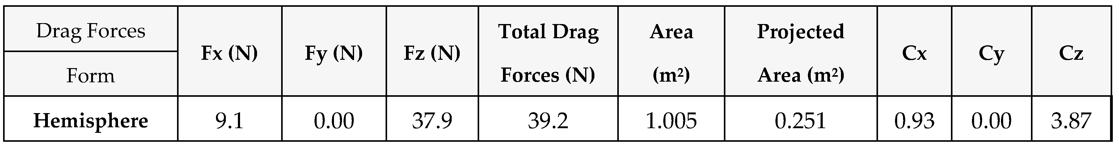
As another symmetrical form, a hemisphere shape is selected as an independent shape of wind direction. The geometry of the hemisphere is shown in Figure 25. The computational mesh became independent in 3,202,462 cells. Due to seven vertical probe lines, Cp-variation is plotted on the surface (Figure 26.), so the upper and lower value of Cp from positive to negative can be observed clearly. The maximum suction values become happened at the top middle point while for the downwind zones, and in other area the suction value is decreasing. Similarly, the variation of mean wind pressure Cp is investigated for horizontal line probes that changed approximately periodically from positive to negative value through normalized distance (Figure 27).
Therefore, as the probe line gets distance from the center point of the hemisphere, the amount of Cp is going to decrease. The Cp contour for hemisphere in Figure 28 shows pressure and suction zone obviously. Finally, in Table 7, the amount of drag forces and wind coefficients are calculated for all global directions using a single simulation as well.
4. Conclusions
In the current study, comprehensive wind simulation is investigated for several forms of tensile surface and classical shapes by using CFD simulation in RWIND Simulation. Steady RANS turbulence models are employed to validate double-curved form due to experimental wind tunnel test and subsequent examples. The process of nonlinear form-finding analysis was performed in RFEM to reach the final shapes of the orthotropic membrane surface. The standard type of form-finding analysis was used for tensile ridge valley and saddle form, and projection type for conical shape. The results included average Cp-distribution through horizontal and vertical probe lines, the contour of mean wind pressure coefficient, and table of drag forces and wind coefficient. For non-symmetric forms θ=0,15,30,45,60,75,90 ͦ have been carried out to evaluate the effect of different angles on Cp-variations. On the other hand, the rest of the forms like the Conical tensile surface, cylindrical, and hemisphere form are independent of wind directions; therefore, based on one simulation and seven horizontal and vertical probe lines, the effect of rotation was investigated to cover Cp-variation of the surface. This study would be applicable for tensile membrane forms that are not covered by standard codes and represent a useful view of wind load design of non-regular shapes. Also, Cp-distribution diagrams can help to estimate the upper and lower value of average wind pressure throw different wind angles attacks.
Acknowledgment
The authors greatly appreciate the support of Dlubal Software for providing RFEM and RWIND Simulation license.
References
- Forster, B. and M. Mollaert, European design guide for tensile surface structures: TensiNet. 2004: TensiNet.
- Engineers, A.S.o.C. Tensile Membrane Structures. 2016. American Society of Civil Engineers.
- Holmes, J. and G. Wood, The determination of structural wind loads for the roofs of several venues for the 2000 Olympics, in Structures 2001: A Structural Engineering Odyssey. 2001. p. 1-21.
- Sun, X., R. Yu, and Y. Wu, Investigation on wind tunnel experiments of ridge-valley tensile membrane structures. Eng. Struct. 2019, 187, 280–298. [Google Scholar] [CrossRef]
- Colliers, J.; et al. , Prototyping of thin shell wind tunnel models to facilitate experimental wind load analysis on curved canopy structures. J. Wind. Eng. Ind. Aerodyn. 2019, 18, 308–322. [Google Scholar] [CrossRef]
- Rizzo, F. and F. Ricciardelli, Design pressure coefficients for circular and elliptical plan structures with hyperbolic paraboloid roof. Eng. Struct. 2017, 139, 153–169. [Google Scholar]
- Bartko, M., S. Molleti, and A. Baskaran, In situ measurements of wind pressures on low slope membrane roofs. J. Wind Eng. Ind. Aerodyn. 2016, 153, 78–91. [Google Scholar]
- Chavez, M.; et al. , Effect of assembly construction on the wind induced pressure of membrane roofs. Eng. Struct. 2020, 221, 110725. [Google Scholar] [CrossRef]
- Dong, X. and J. Ye, The point and area-averaged wind pressure influenced by conical vortices on saddle roofs. J. Wind Eng. Ind. Aerodyn. 2012, 101, 67–84. [Google Scholar]
- Singh, J. and A. K. Roy, Effects of roof slope and wind direction on wind pressure distribution on the roof of a square plan pyramidal low-rise building using CFD simulation. Int. J. Adv. Struct. Eng. 2019, 11, 231–254. [Google Scholar]
- Oyejobi, D., M. Jameel, and N.R. Sulong, Nonlinear response of tension leg platform subjected to wave, current and wind forces. Int. J. Civ. Eng. 2016, 14, 521–533. [Google Scholar] [CrossRef]
- Colliers, J.; et al. , Mean pressure coefficient distributions over hyperbolic paraboloid roof and canopy structures with different shape parameters in a uniform flow with very small turbulence. Eng. Struct. 2020, 205, 110043. [Google Scholar] [CrossRef]
- Nagai, Y.; et al. , Wind Response of Horn-shaped Membrane Roof and Proposal of Gust Effect Factor For Membrane Structure. J. Int. Assoc. Shell Spat. Struct. 2012, 53, 169–176. [Google Scholar]
- Hincz, K. and M. Gamboa-Marrufo, Deformed shape wind analysis of tensile membrane structures. J. Struct. Eng. 2016, 142, 04015153. [Google Scholar] [CrossRef]
- Liu, M., X. Chen, and Q. Yang, Characteristics of dynamic pressures on a saddle type roof in various boundary layer flows. J. Wind Eng. Ind. Aerodyn. 2016, 150, 1–14. [Google Scholar] [CrossRef]
- Zhou, X.; et al. , Research on wind-induced responses of a large-scale membrane structure. Earthq. Eng. Eng. Vib. 2013, 12, 297–305. [Google Scholar] [CrossRef]
- Mall, F. Ermittlung von Windlasten auf Bauwerke mit Hilfe von CFD-Berechnungen. 2014, Master Thesis, Hochschule für Technik, Wirtschaft und Gestaltung Konstanz ….
- Michalski, A. , Simulation leichter Flächentragwerke in einer numerisch generierten atmosphärischen Grenzschicht. 2010, Technische Universität München.
- Blanco, S.J.P. and K. Hincz, Comput. Wind Eng. A Mast-Support. Tensile Structure. Period. Polytech. Civ. Eng. 2022, 66, 210–219. [Google Scholar]
- Franke, J. Recommendations of the COST action C14 on the use of CFD in predicting pedestrian wind environment. in The fourth international symposium on computational wind engineering, Yokohama, Japan. 2006. Citeseer.
- Tominaga, Y.; et al. , AIJ guidelines for practical applications of CFD to pedestrian wind environment around buildings. J. Wind Eng. Ind. Aerodyn. 2008, 96, 1749–1761. [Google Scholar] [CrossRef]
- Versteeg, H.K. and W. Malalasekera, An introduction to computational fluid dynamics: The finite volume method. 2007: Pearson education.
- Hu, P.; et al. , Numerical simulation of the neutral equilibrium atmospheric boundary layer using the SST k-omega turbulence model. Wind Struct. 2013, 17, 87–105. [Google Scholar] [CrossRef]
- Toparlar, Y.; et al. , A review on the CFD analysis of urban microclimate. Renew. Sustain. Energy Rev. 2017, 80, 1613–1640. [Google Scholar] [CrossRef]
- Montazeri, H. and B. Blocken, CFD simulation of wind-induced pressure coefficients on buildings with and without balconies: Validation and sensitivity analysis. Build. Environ. 2013, 60, 137–149. [Google Scholar]
- Menter, F.R. , Two-equation eddy-viscosity turbulence models for engineering applications. AIAA J. 1994, 32, 1598–1605. [Google Scholar] [CrossRef]
- Kim, R.-w., I. -b. Lee, and K.-s. Kwon, Evaluation of wind pressure acting on multi-span greenhouses using CFD technique, Part 1: Development of the CFD model. Biosyst. Eng. 2017, 164, 235–256. [Google Scholar]
- Malizia, F., H. Montazeri, and B. Blocken, CFD simulations of spoked wheel aerodynamics in cycling: Impact of computational parameters. J. Wind Eng. Ind. Aerodyn. 2019, 194, 103988. [Google Scholar]
- Lee, M.-H., Y. -C. Shiah, and C.-J. Bai, Experiments and numerical simulations of the rotor-blade performance for a small-scale horizontal axis wind turbine. J. Wind Eng. Ind. Aerodyn. 2016, 149, 17–29. [Google Scholar] [CrossRef]
- Otto, F. and B. Rasch, Finding Form, Deutscher Werkbund Bayern, Edition A. 1995, Menges.
- Bletzinger, K.-U. and E. Ramm, A general finite element approach to the form finding of tensile structures by the updated reference strategy. Int. J. Space Struct. 1999, 14, 131–145. [Google Scholar] [CrossRef]
- Bletzinger, K.-U. and E. Ramm, Structural optimization and form finding of light weight structures. Comput. Struct. 2001, 79, 2053–2062. [Google Scholar]
- En, B. , Eurocode 1: Actions on Structures—Part 1–4: General Actions—Wind Actions. NA to BS EN, Brussels, Belgium, 1991.
- 34. ASCE. ASCE/SEI 7-16. Minimum design loads and associated criteria for buildings and other structures.
- Canada, N.R.C.o. , National Building Code of Canada, 2015. 2015: National Research Council Canada.
- Ahsan, M. , Numerical analysis of friction factor for a fully developed turbulent flow using k–ε turbulence model with enhanced wall treatment. Beni-Suef Univ. J. Basic Appl. Sci. 2014, 3, 269–277. [Google Scholar] [CrossRef]
- Motozawa, M.; et al. , Experimental investigation on turbulent structure of drag reducing channel flow with blowing polymer solution from the wall. Flow, turbulence and combustion 2012, 88, 121–141. [Google Scholar] [CrossRef]
- Zhang, C.; et al. , Wind pressure coefficients for buildings with air curtains. J. Wind Eng. Ind. Aerodyn. 2020, 205, 104265. [Google Scholar] [CrossRef]
- Chavez, M.; et al. , Near-field pollutant dispersion in the built environment by CFD and wind tunnel simulations. J. Wind Eng. Ind. Aerodyn. 2011, 99, 330–339. [Google Scholar] [CrossRef]
- Tominaga, Y. and T. Stathopoulos, Numerical simulation of dispersion around an isolated cubic building: Comparison of various types of k–ɛ models. Atmos. Environ. 2009, 43, 3200–3210. [Google Scholar] [CrossRef]
Figure 1.
Flowchart for airflow analysis.
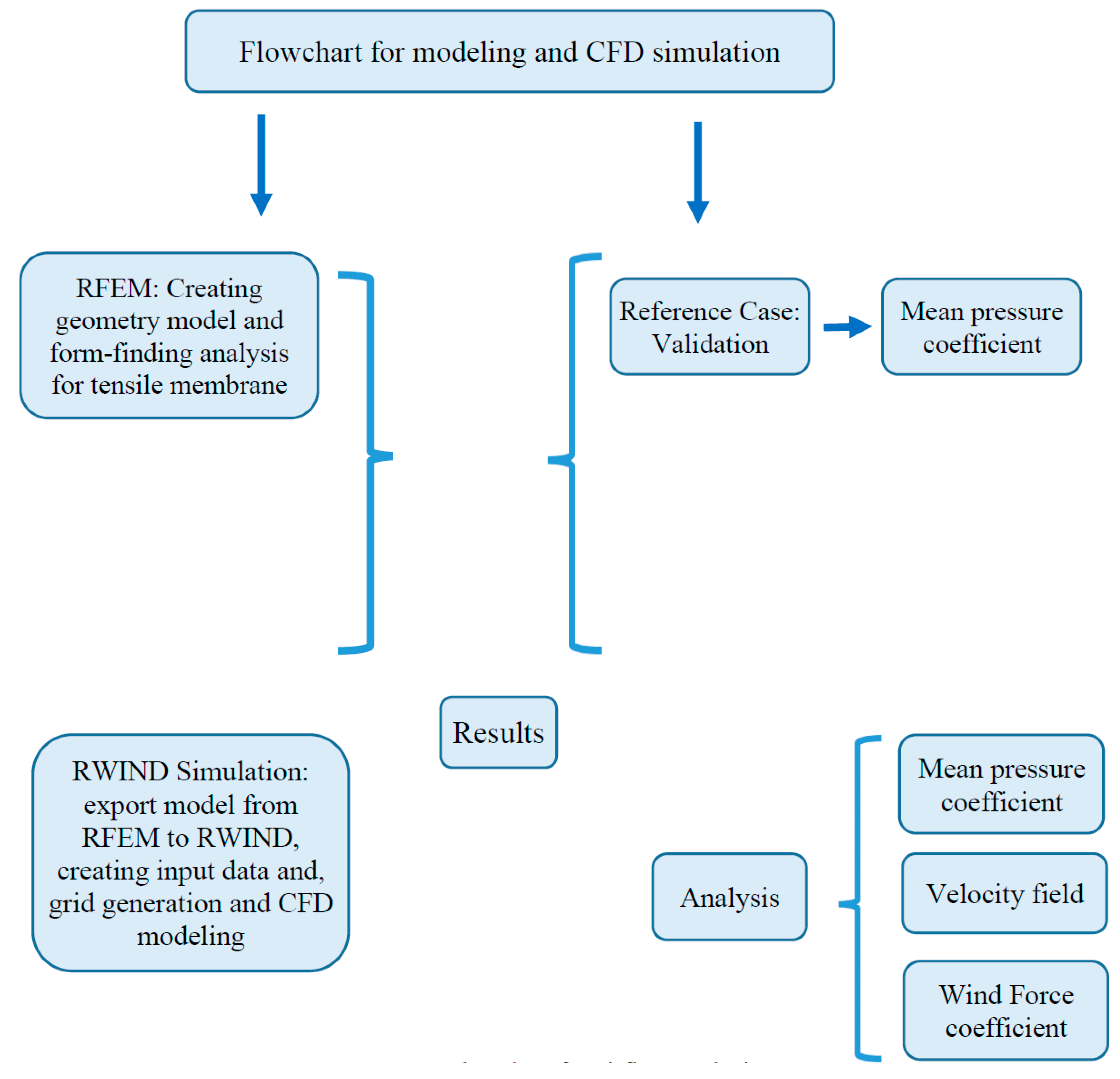
Figure 2.
Dimention of the slightly curved hypar roof.
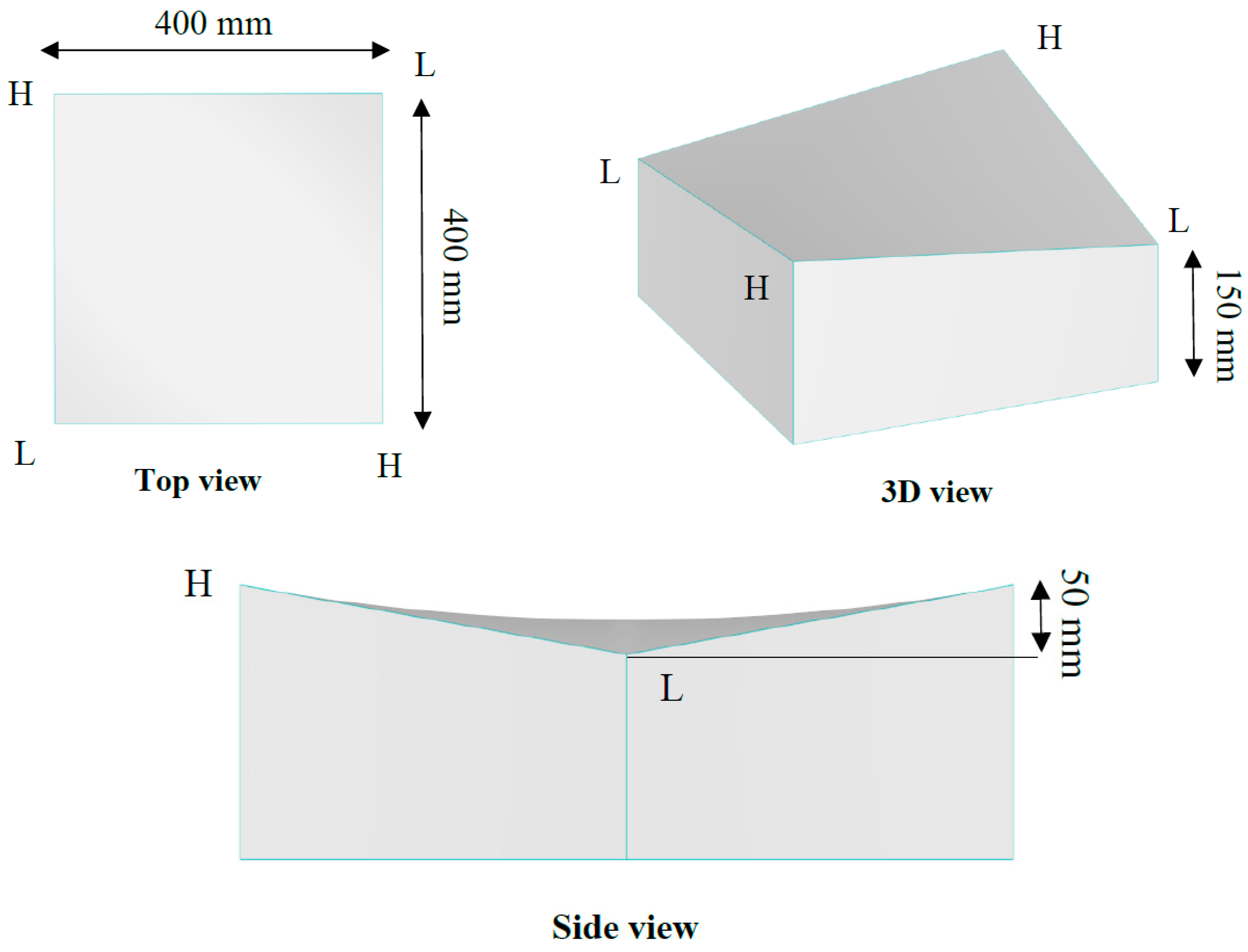
Figure 3.
Profile of wind speed and turbulence intensity due to height.
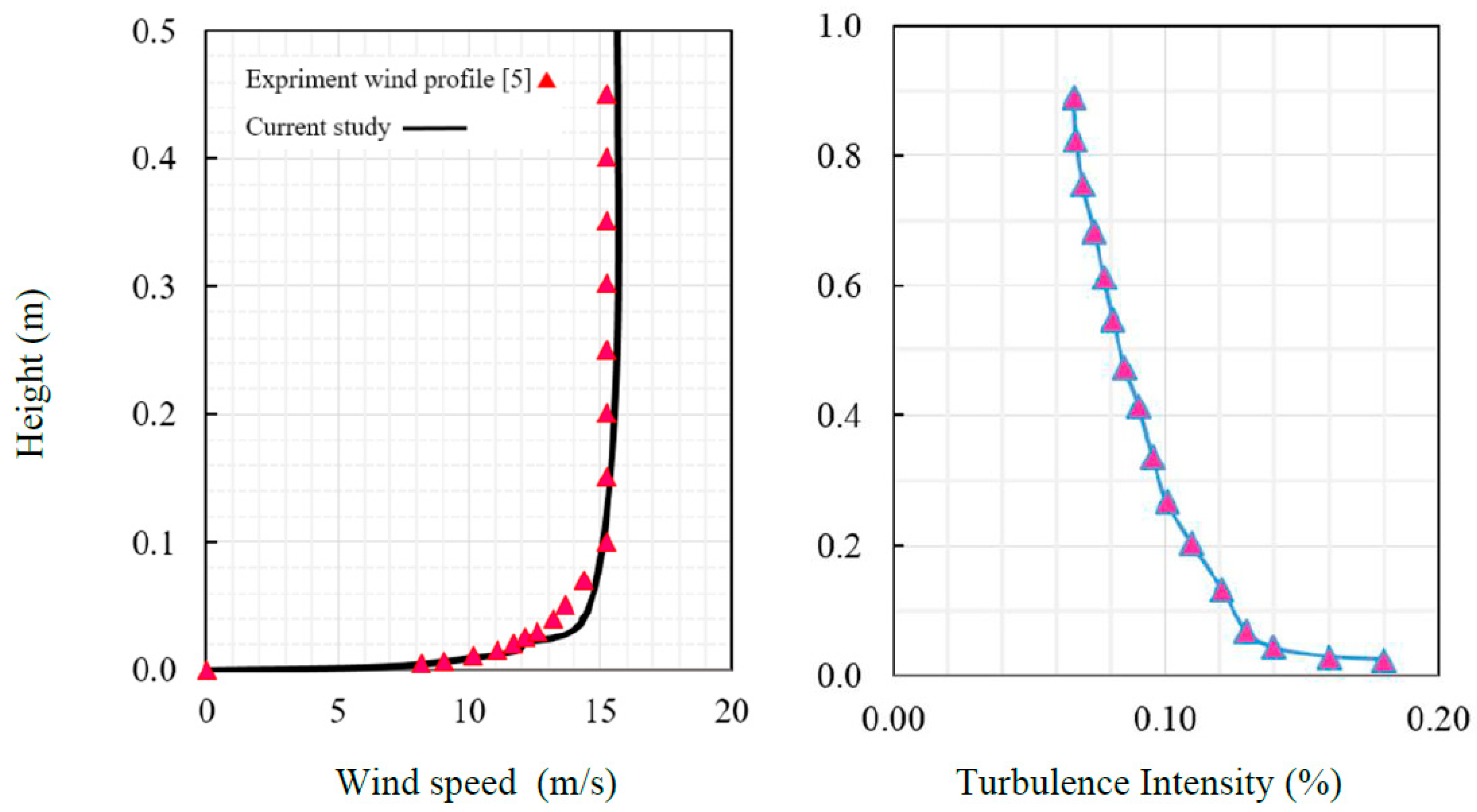
Figure 5.
Mean wind pressure coefficient (Cp,e) over the slightly curved hypar roof (a). Standard k-ε turbulence model (b). SST k-ω turbulence model (c). comparison of mean Cp,e value at the centerline (d). normalized line on the hypar roof.
Figure 5.
Mean wind pressure coefficient (Cp,e) over the slightly curved hypar roof (a). Standard k-ε turbulence model (b). SST k-ω turbulence model (c). comparison of mean Cp,e value at the centerline (d). normalized line on the hypar roof.
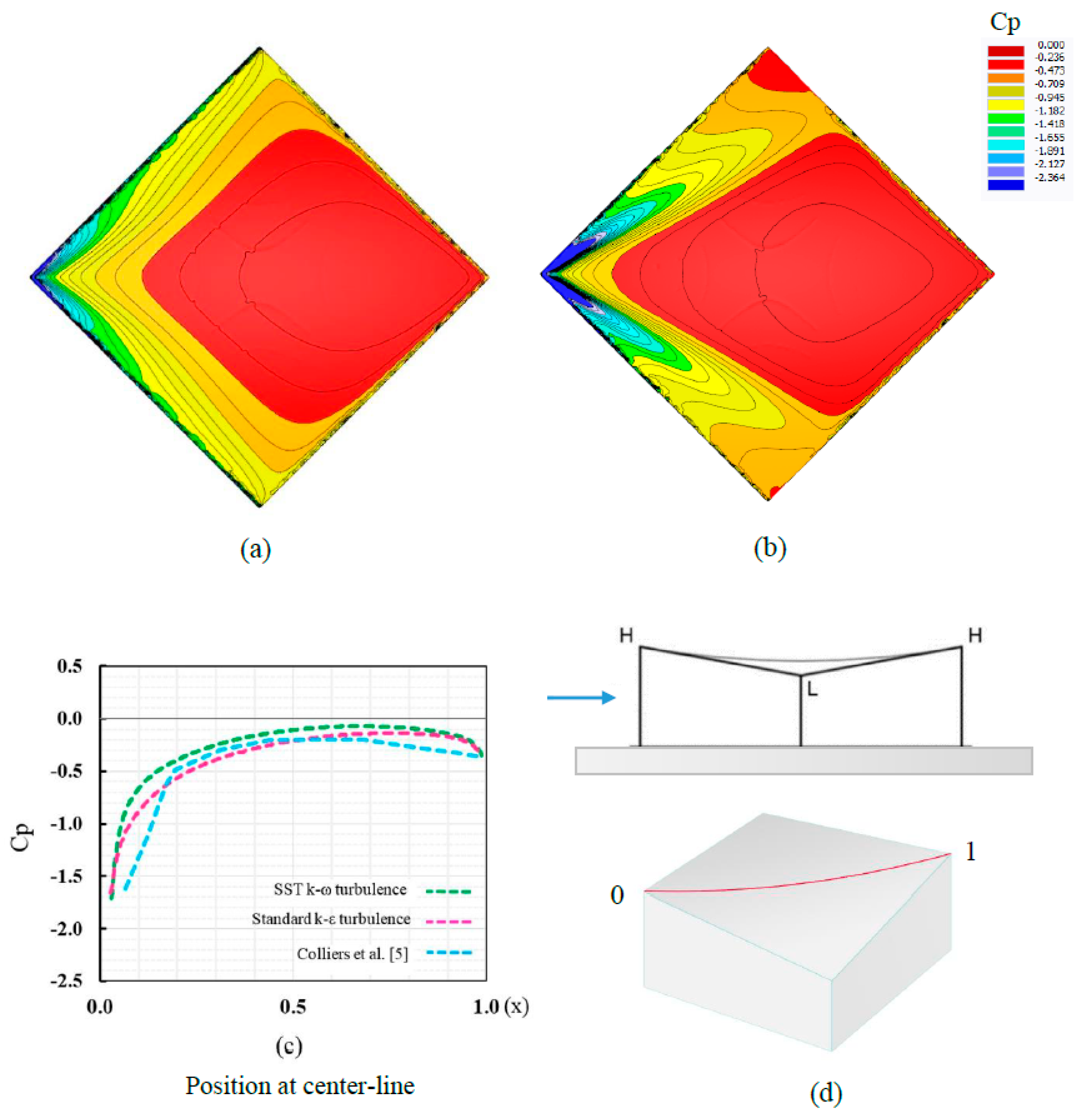
Figure 6.
Grid independency of Cp-distribution for three numbers of elements.
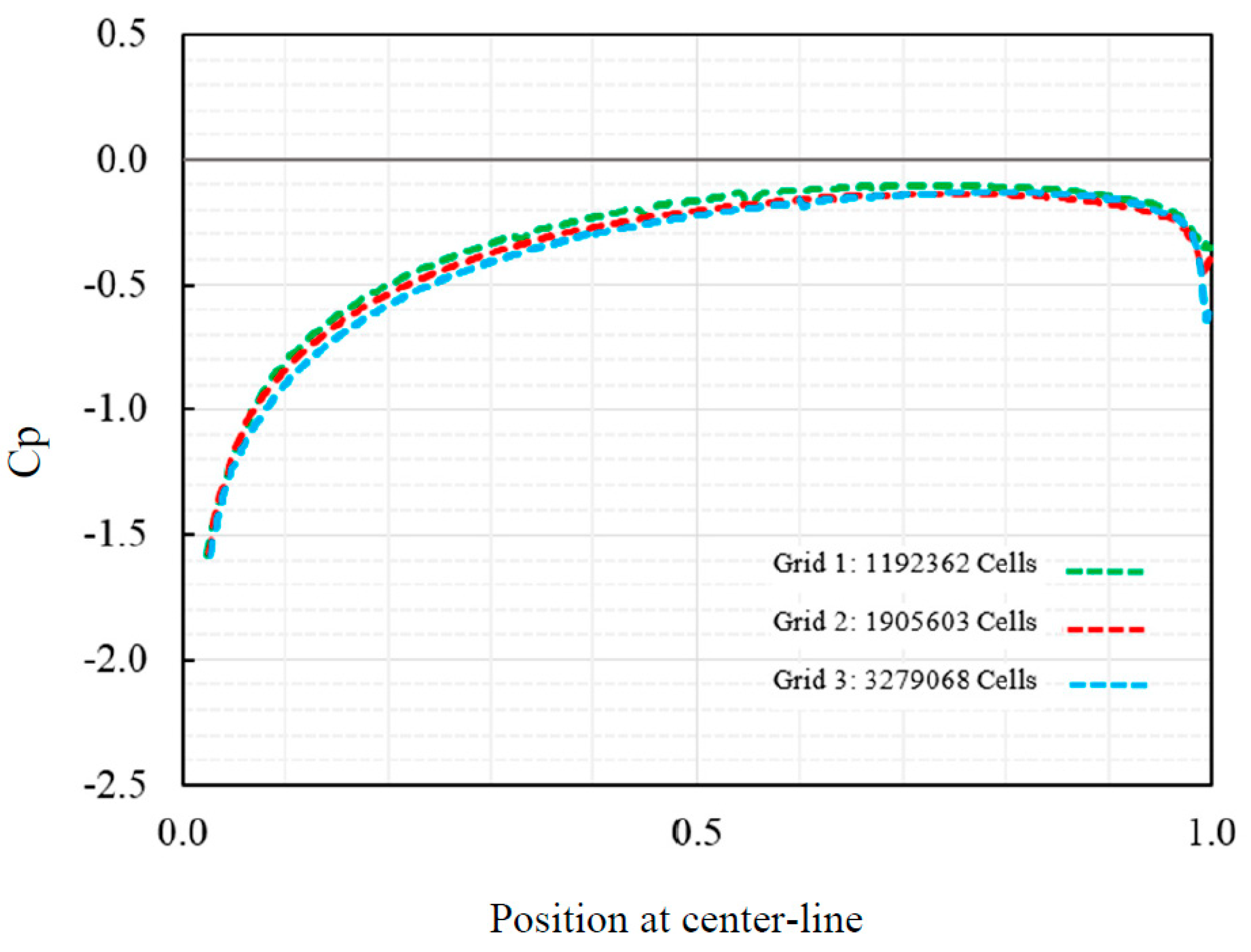
Figure 7.
Conical geometry form in RFEM and FE mesh information.
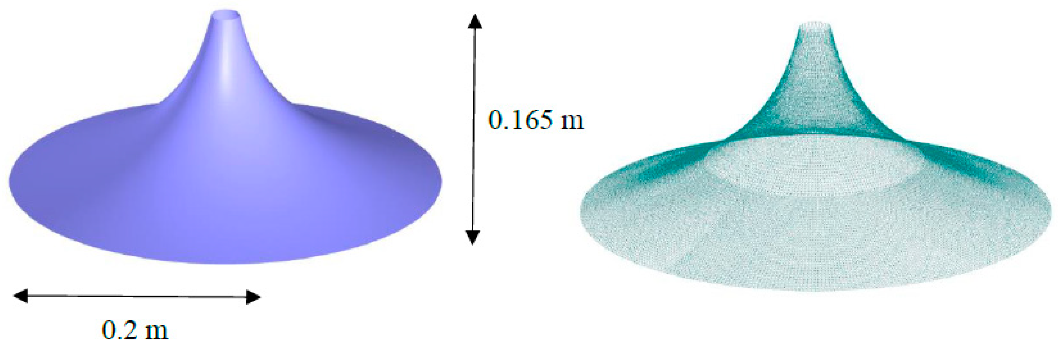
Figure 8.
Average of wind pressure distribution on vertical probe lines for conical form.
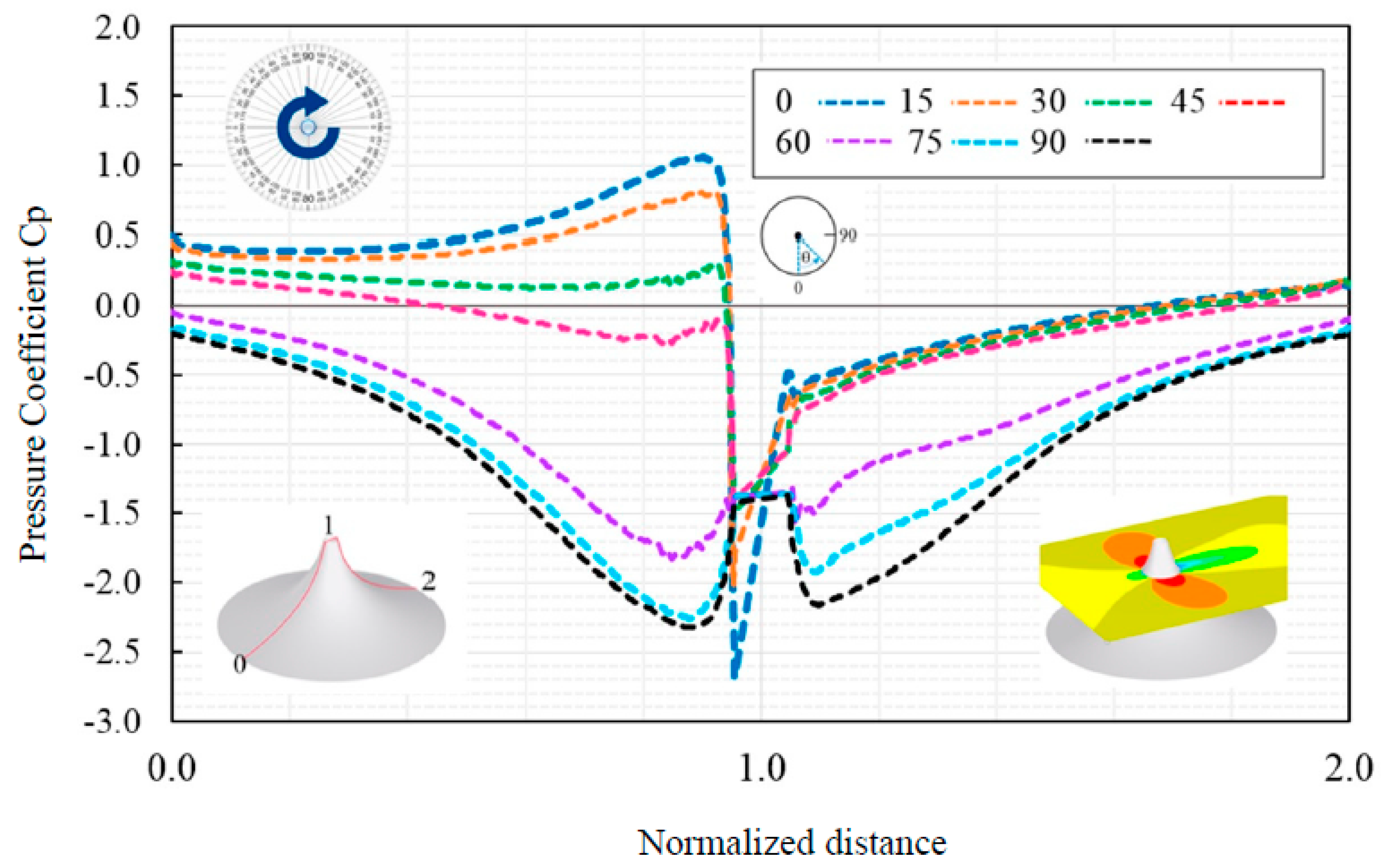
Figure 9.
Average Cp contour for conical form.
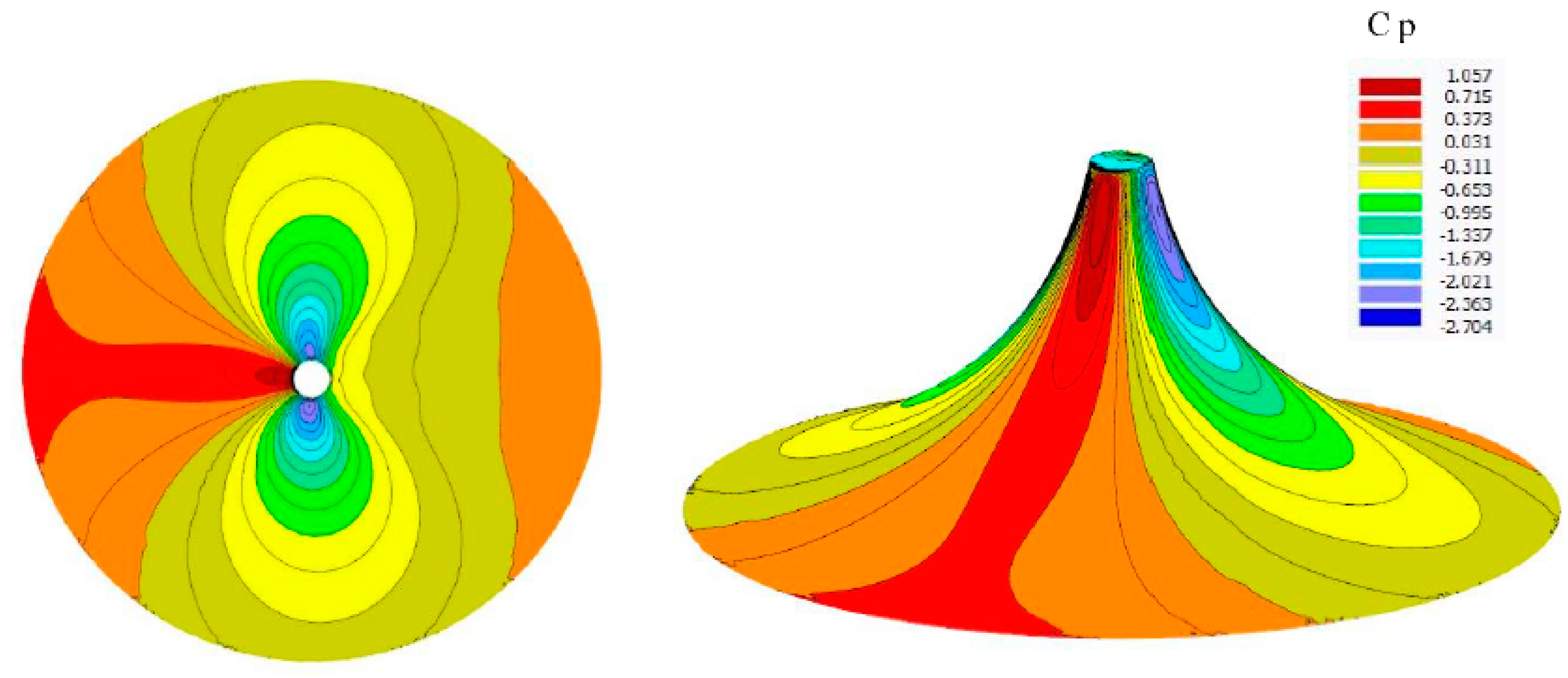
Figure 10.
Average of wind pressure distribution on horizental probe lines for conical form.
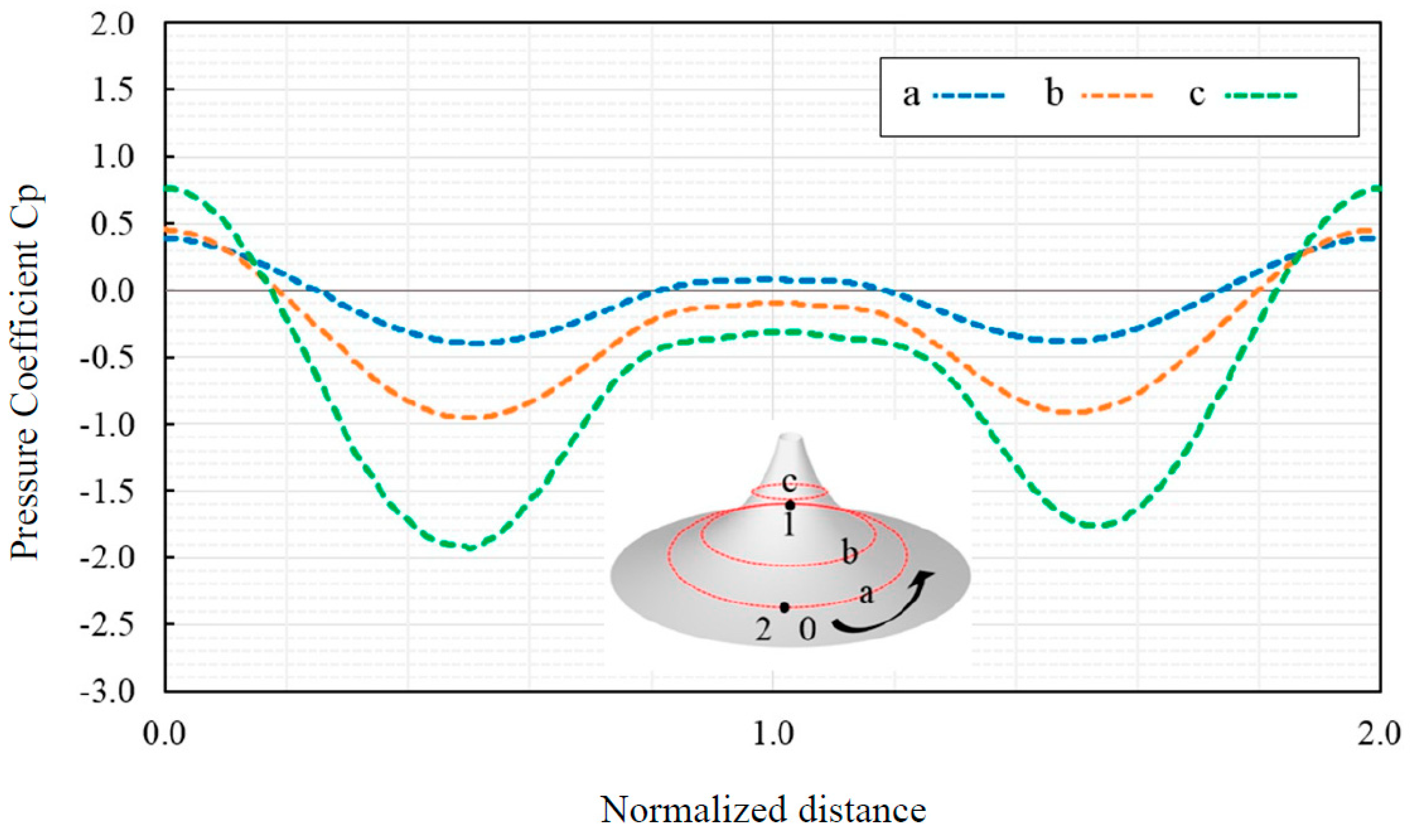
Figure 11.
Tensile ridge-valley form in RFEM and FE mesh information.
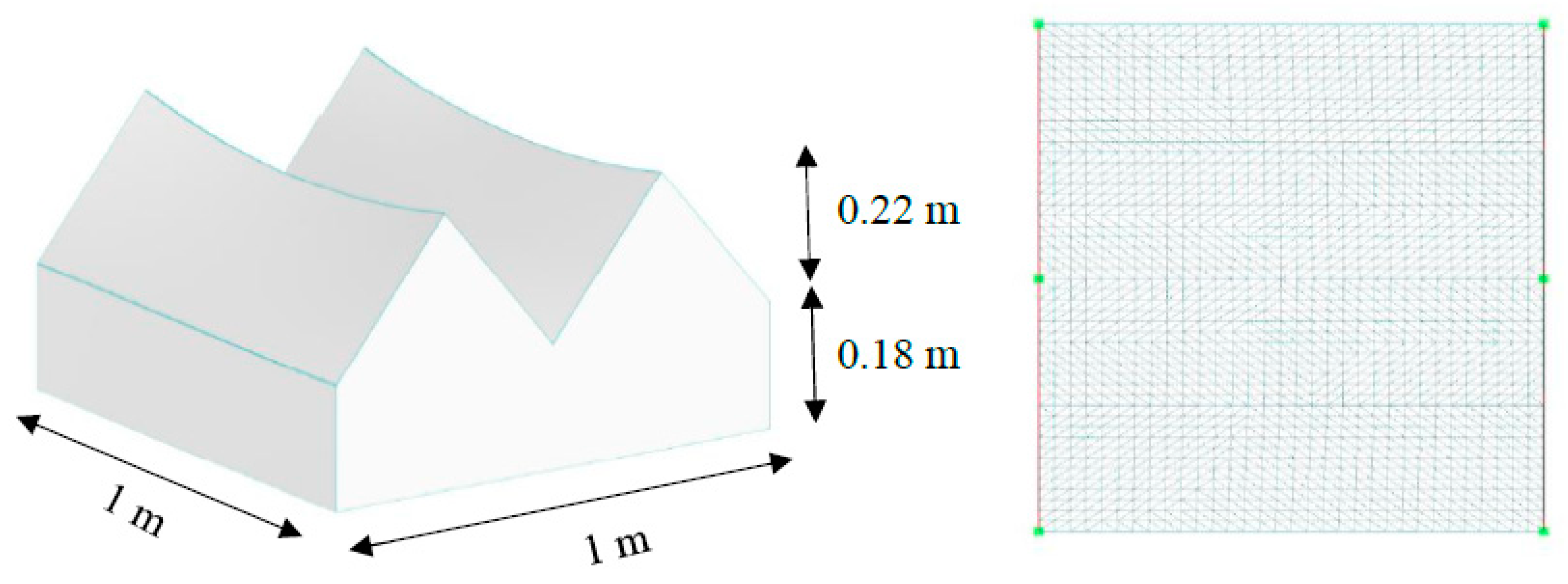
Figure 12.
Average of Cp-distribution on vertical probe lines for tensile ridge-valley.
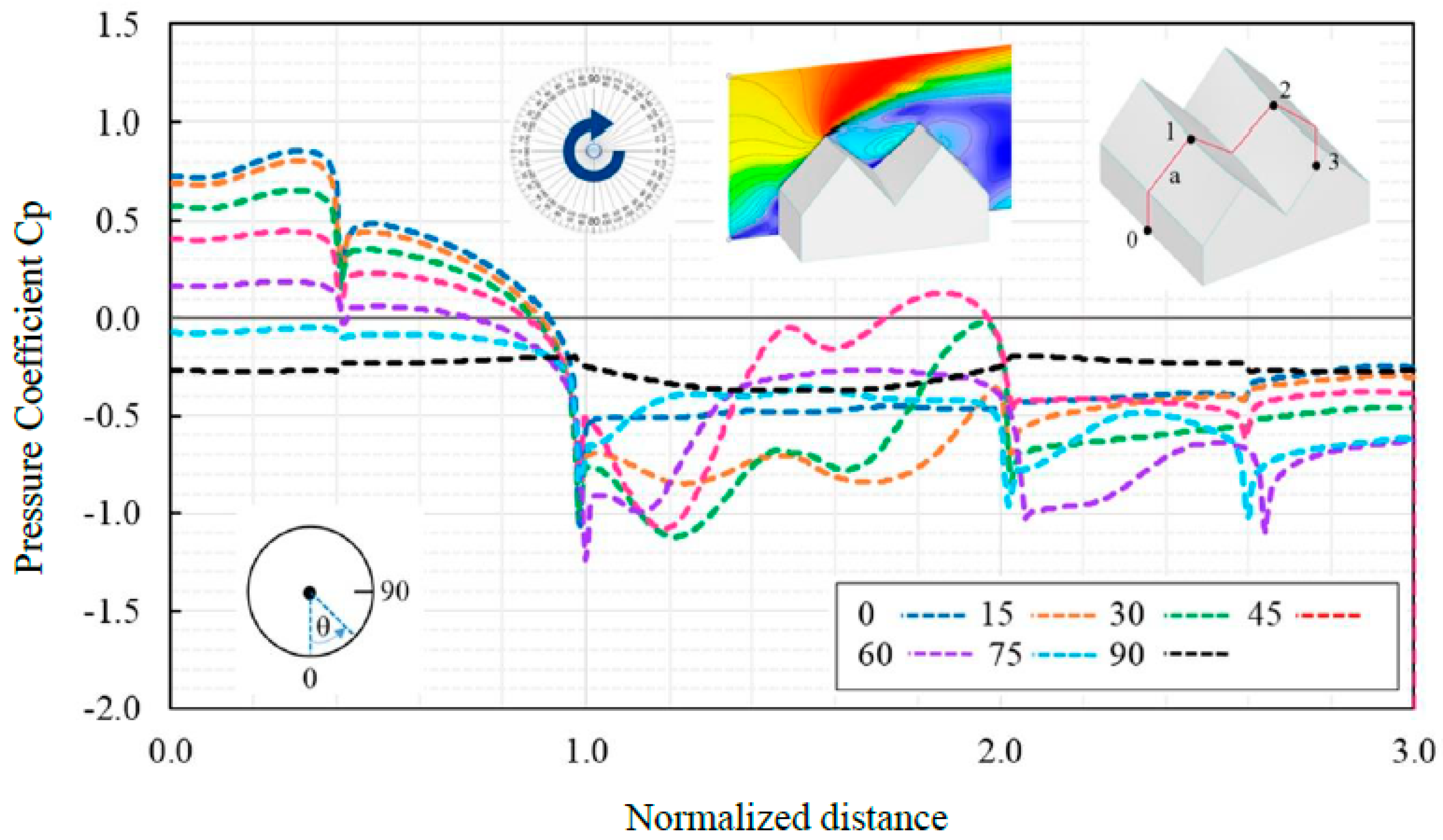
Figure 13.
Average Cp contour for tensile ridge-valley surface.
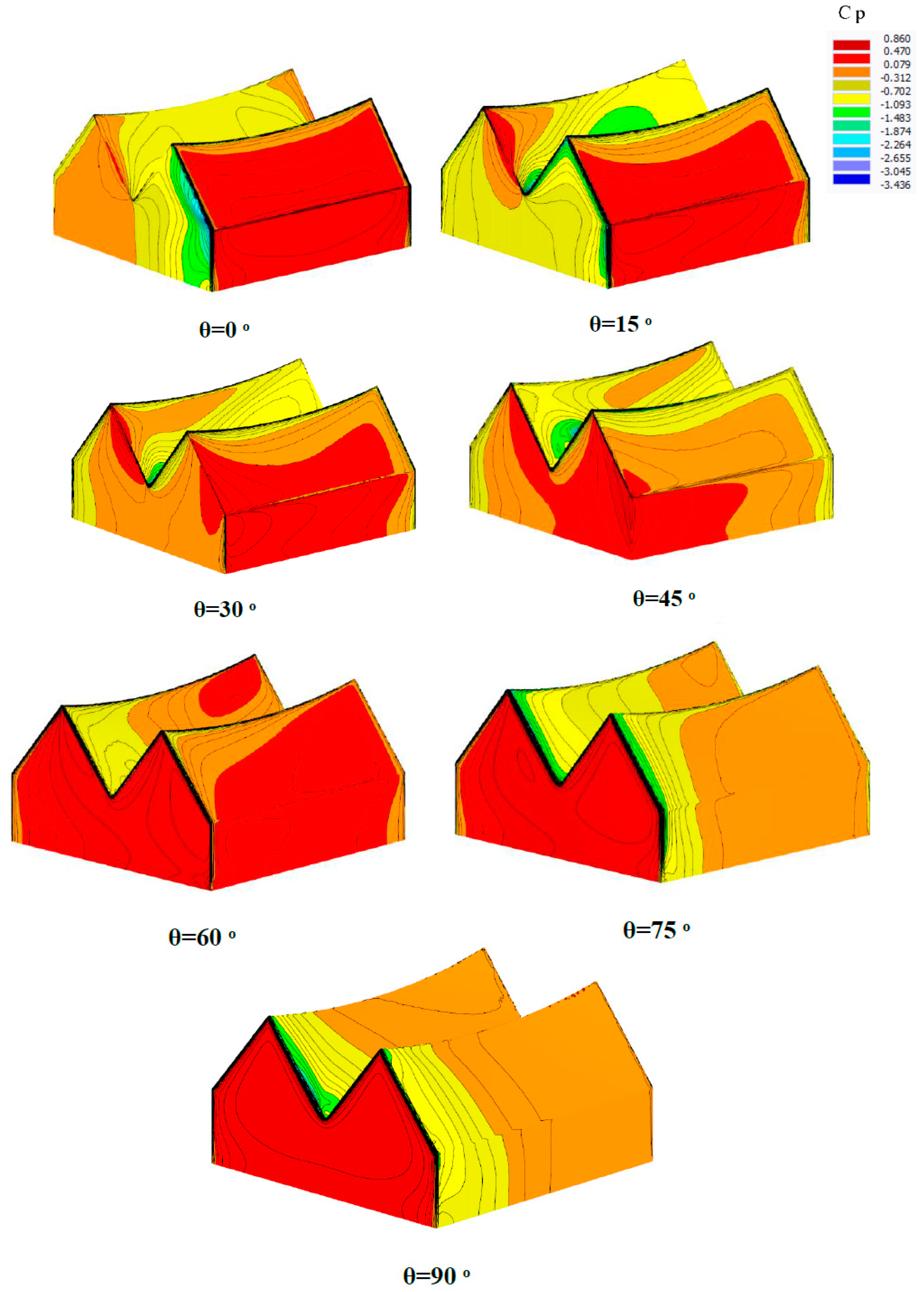
Figure 14.
Saddle geometry information in RFEM and FE mesh data.
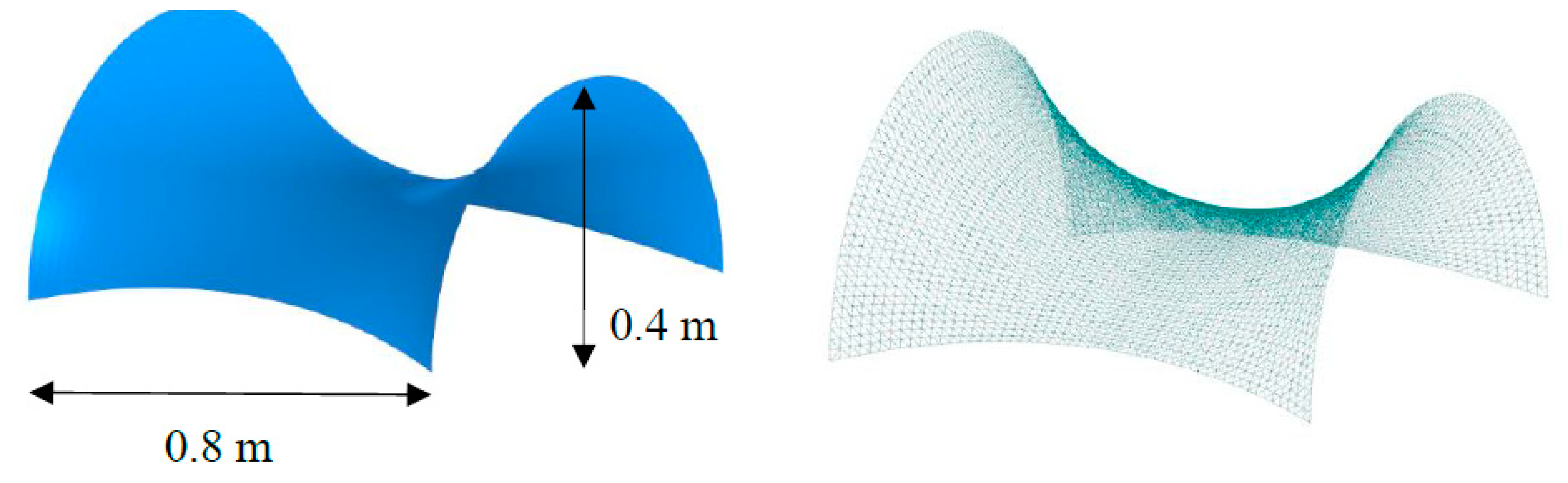
Figure 15.
Average wind pressure distribution on vertical probe lines for saddle shape on θ=0o.
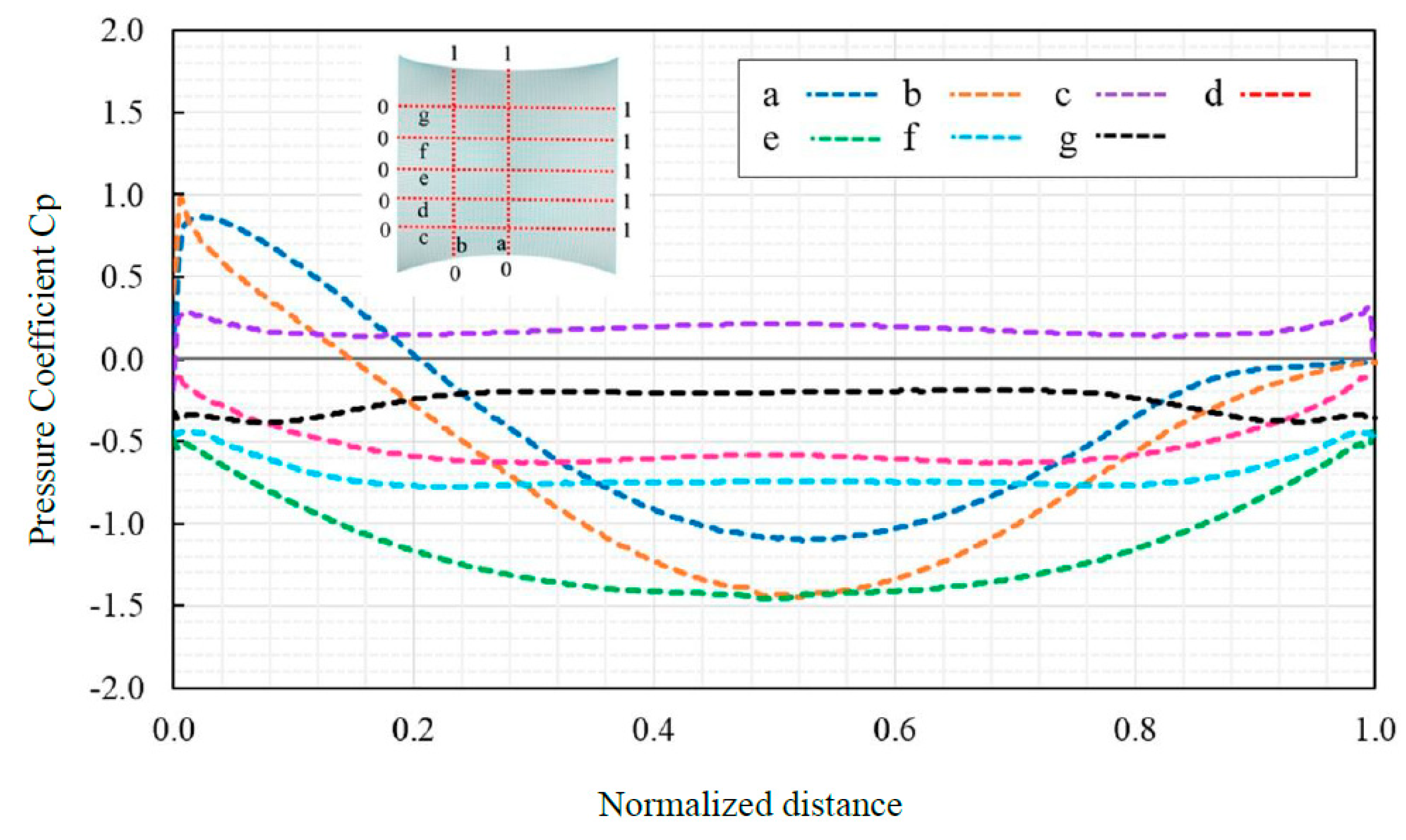
Figure 16.
Average of wind pressure distribution on probe lines for saddle shape.
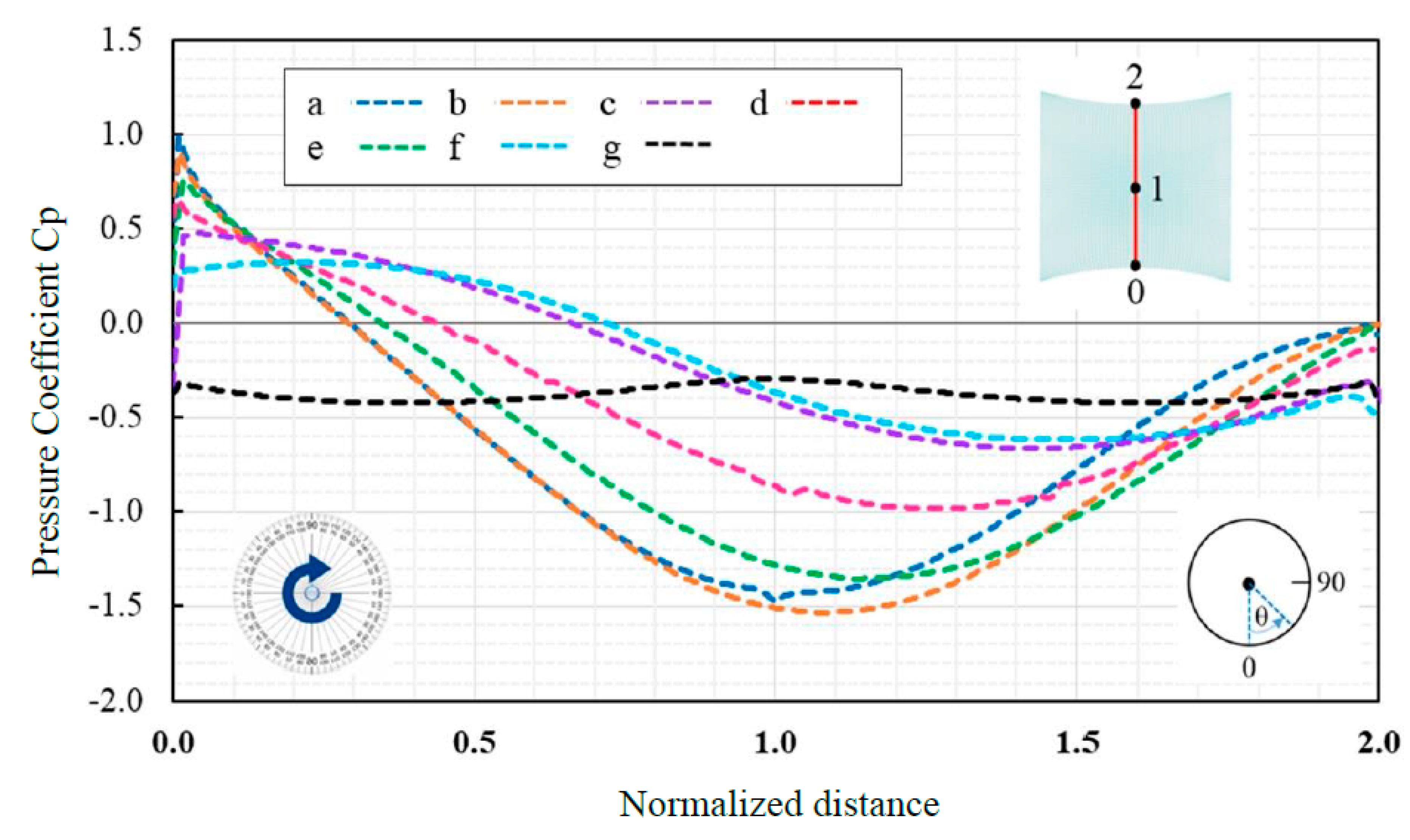
Figure 17.
Average of Cp countour for tensile saddle through 7 wind directions.
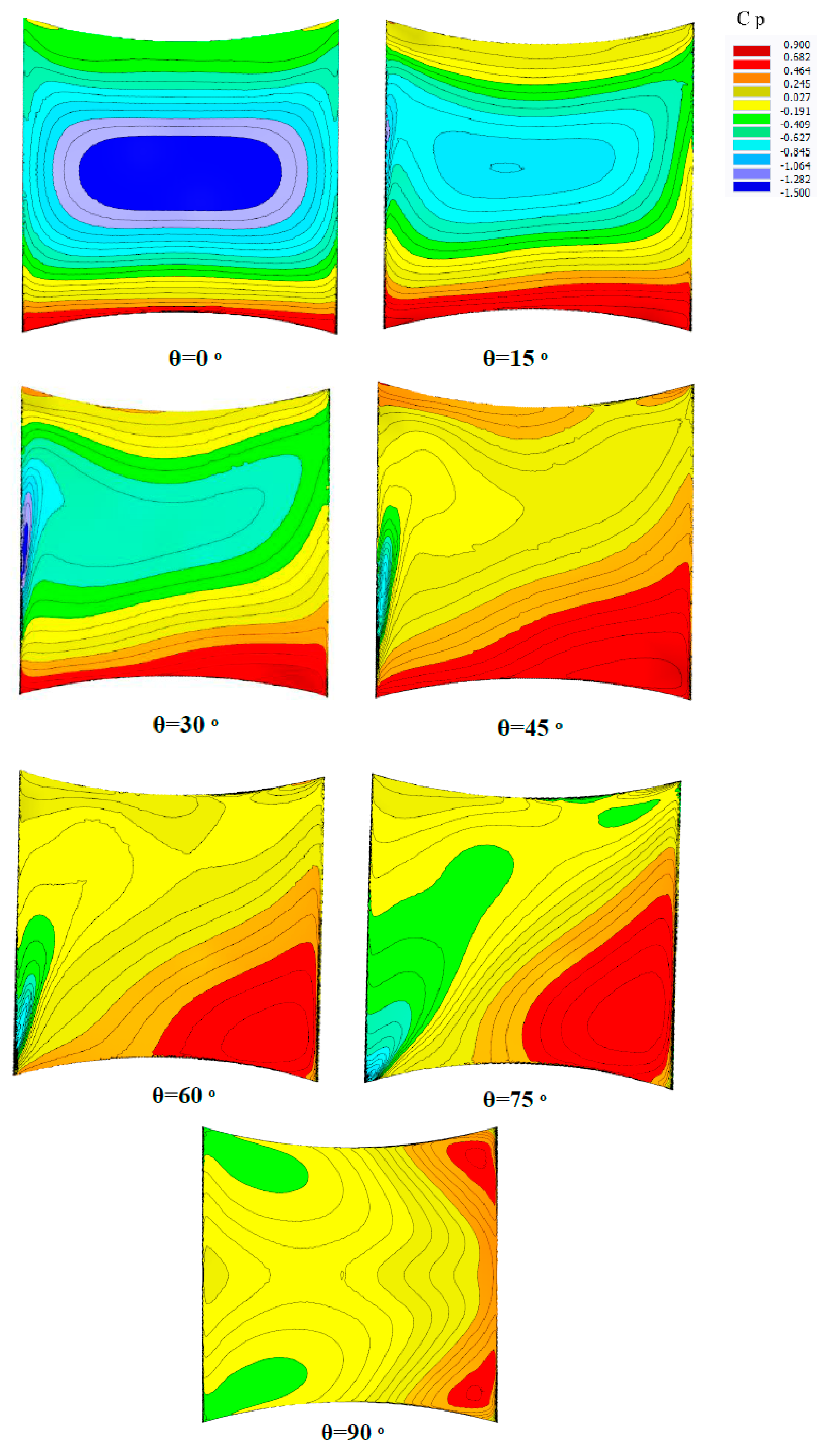
Figure 18.
Cube shape geometry.
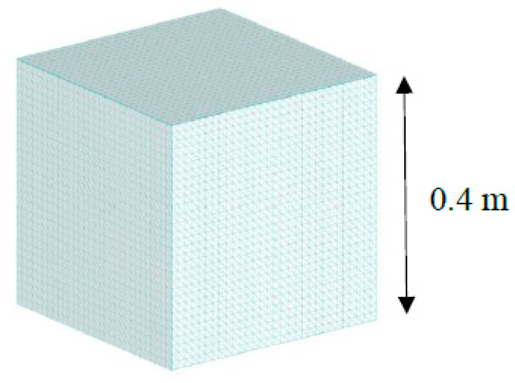
Figure 19.
Average of wind pressure distribution on vertical probe lines for cube shape.
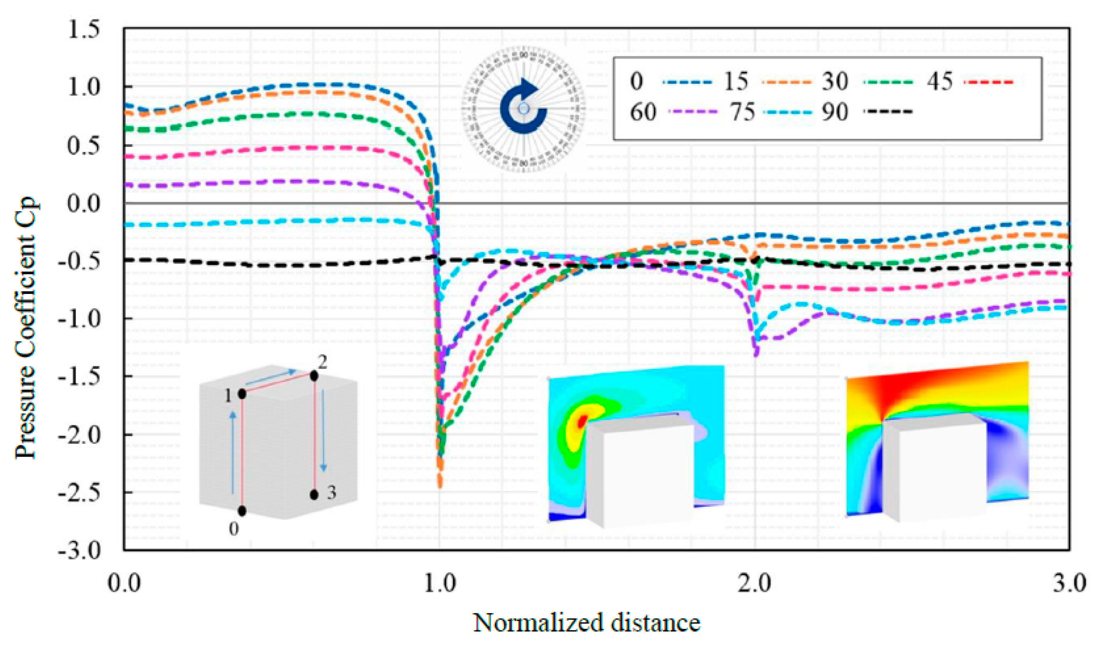
Figure 20.
Average of Cp-distribution for cube form through 7 wind directions.
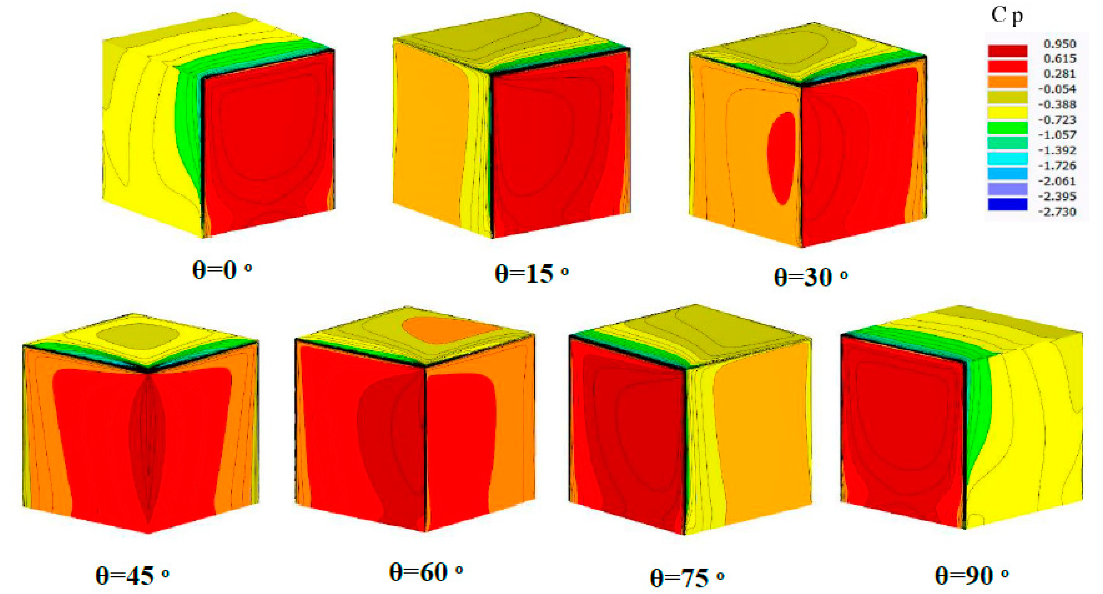
Figure 21.
Cylindrical geometry in RFEM and FE mesh information.
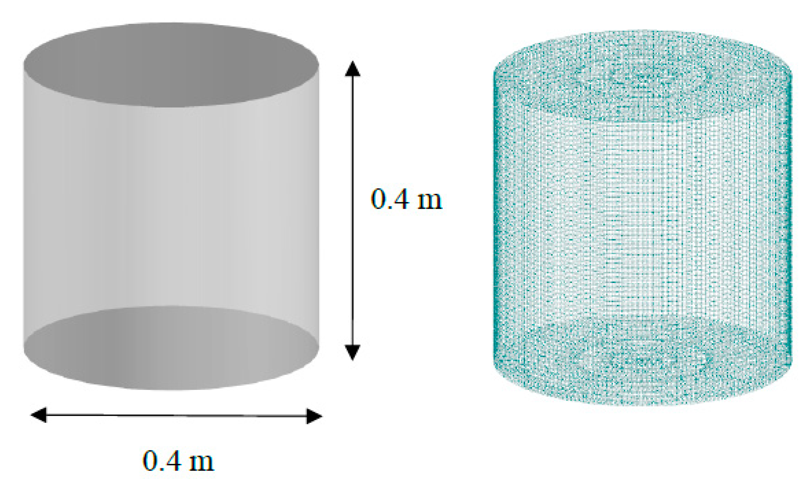
Figure 22.
Average of Cp- distribution for cylindrical form through 7 wind directions.
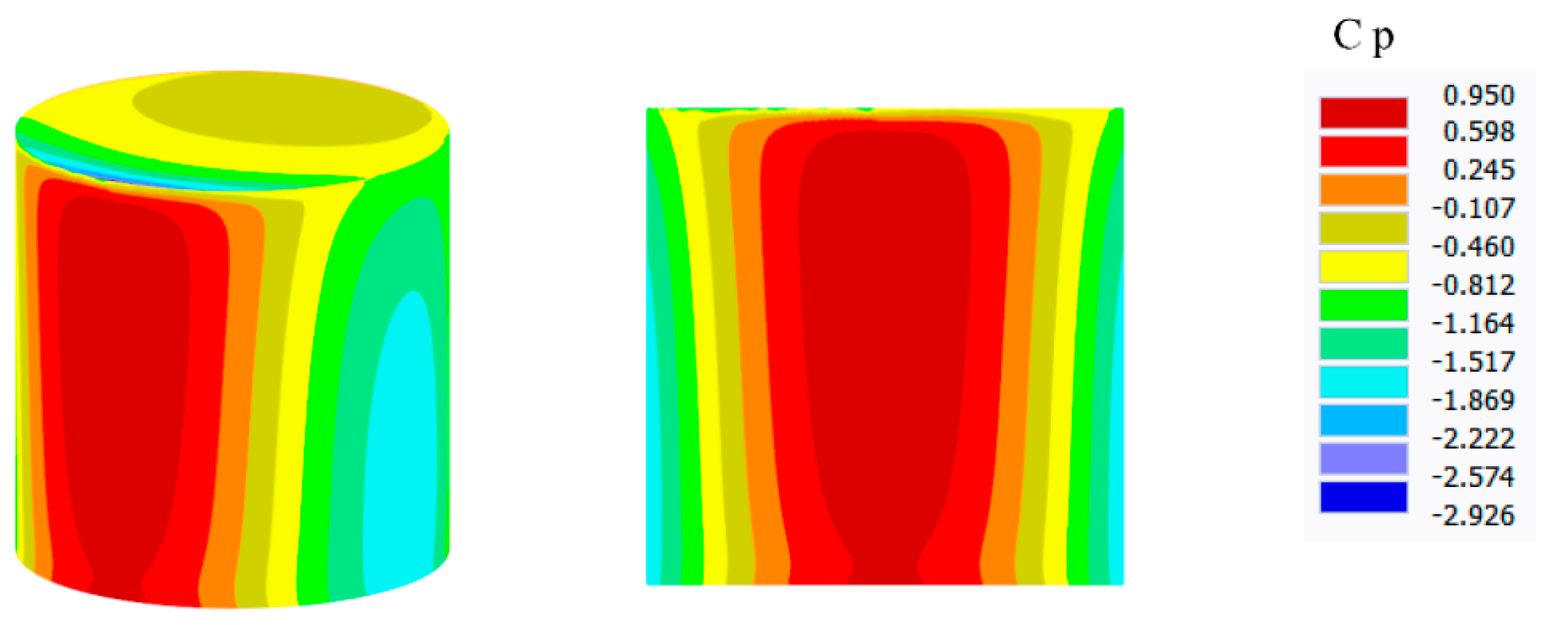
Figure 23.
Average of wind pressure distribution on vertical probe lines for cylindrical shape.
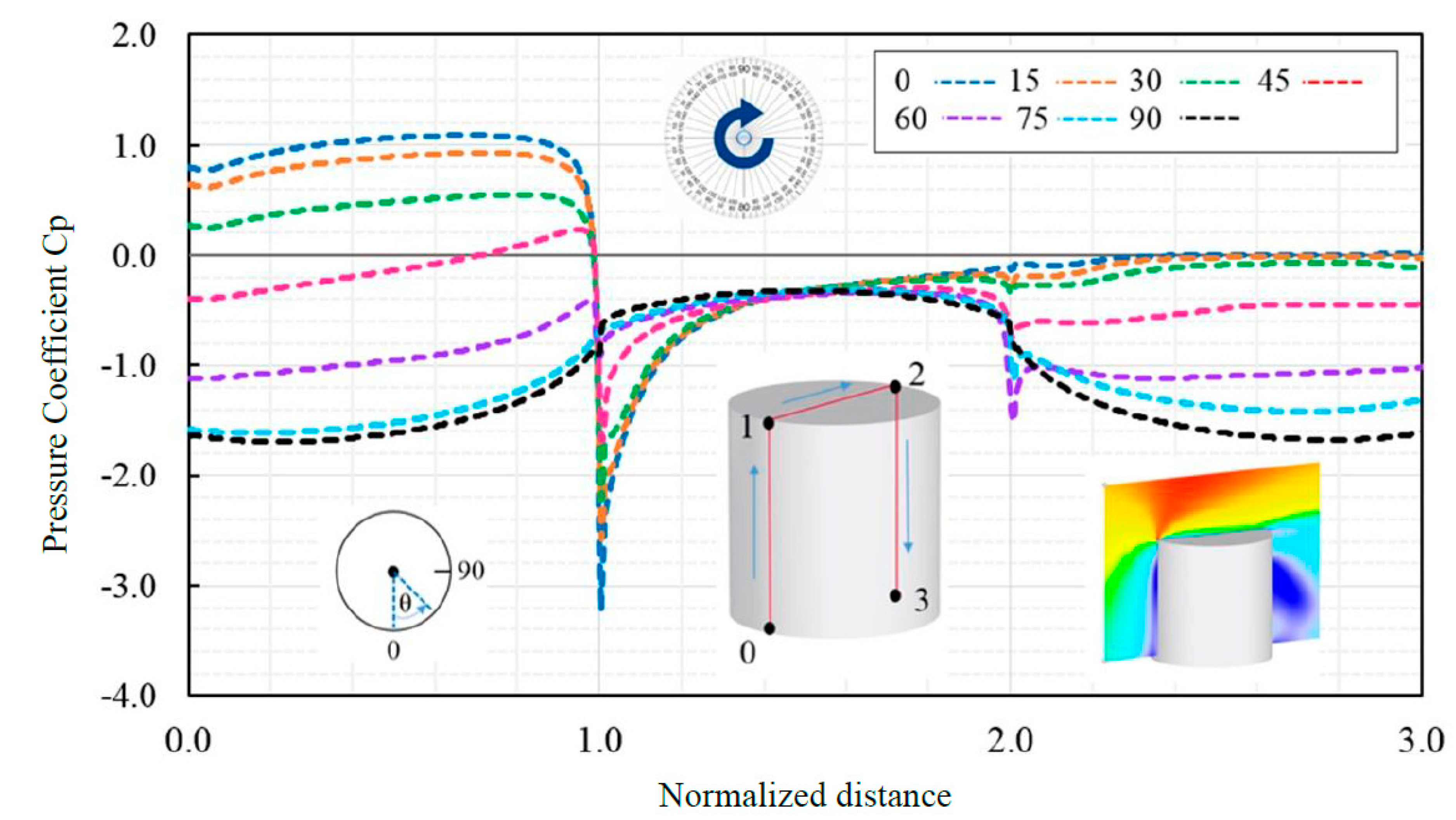
Figure 24.
Average of wind pressure distribution on horizontal probe lines for the cylindrical shape.
Figure 24.
Average of wind pressure distribution on horizontal probe lines for the cylindrical shape.
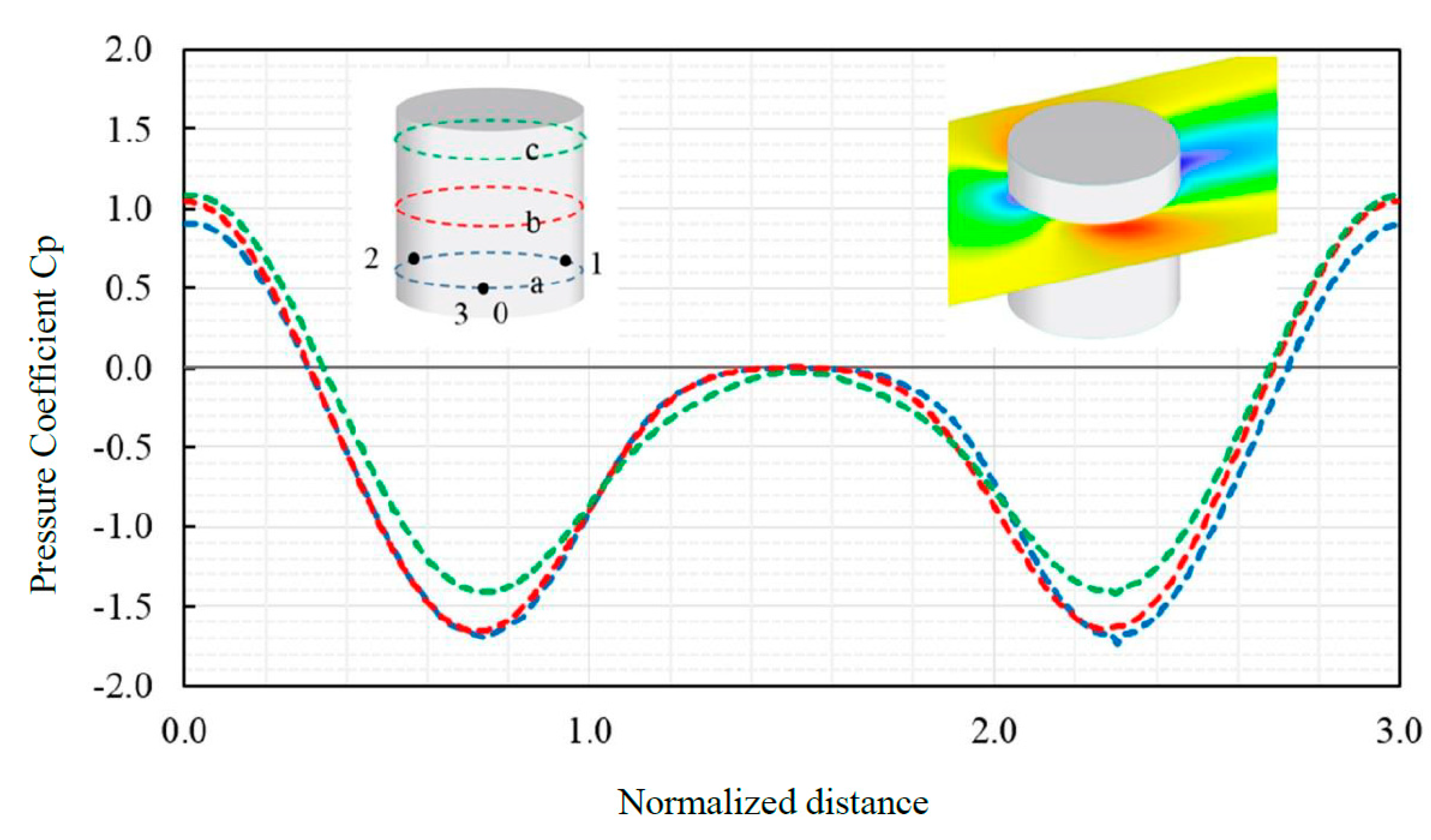
Figure 25.
Hemisphere geometry information in RFEM and FE mesh data.
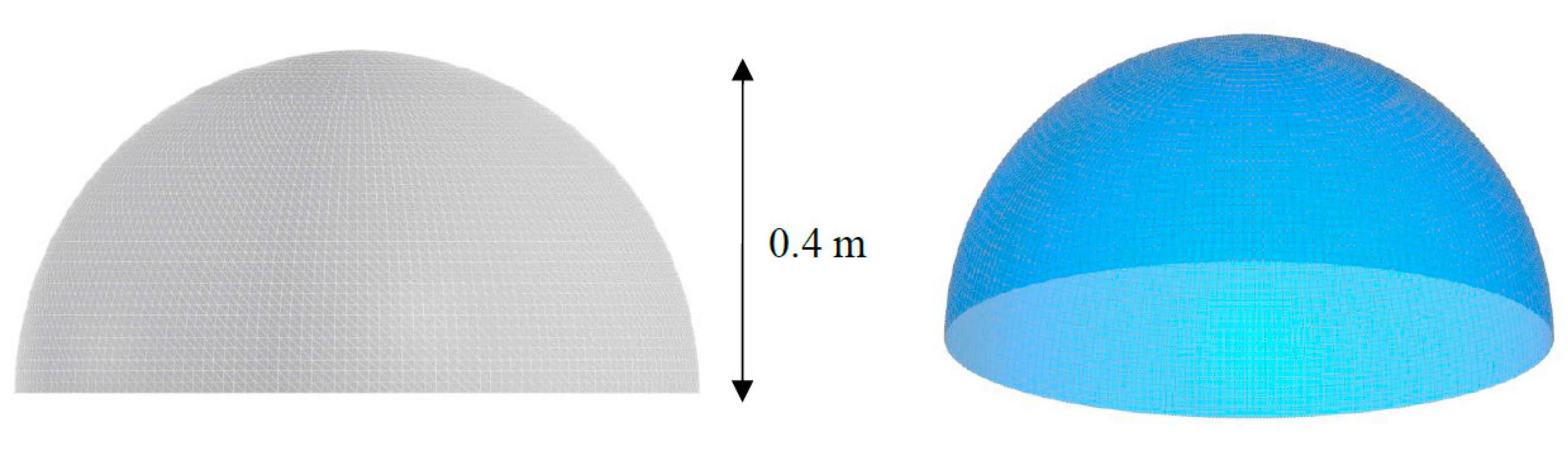
Figure 26.
Average of wind pressure distribution on vertical probe lines for hemisphere shape.
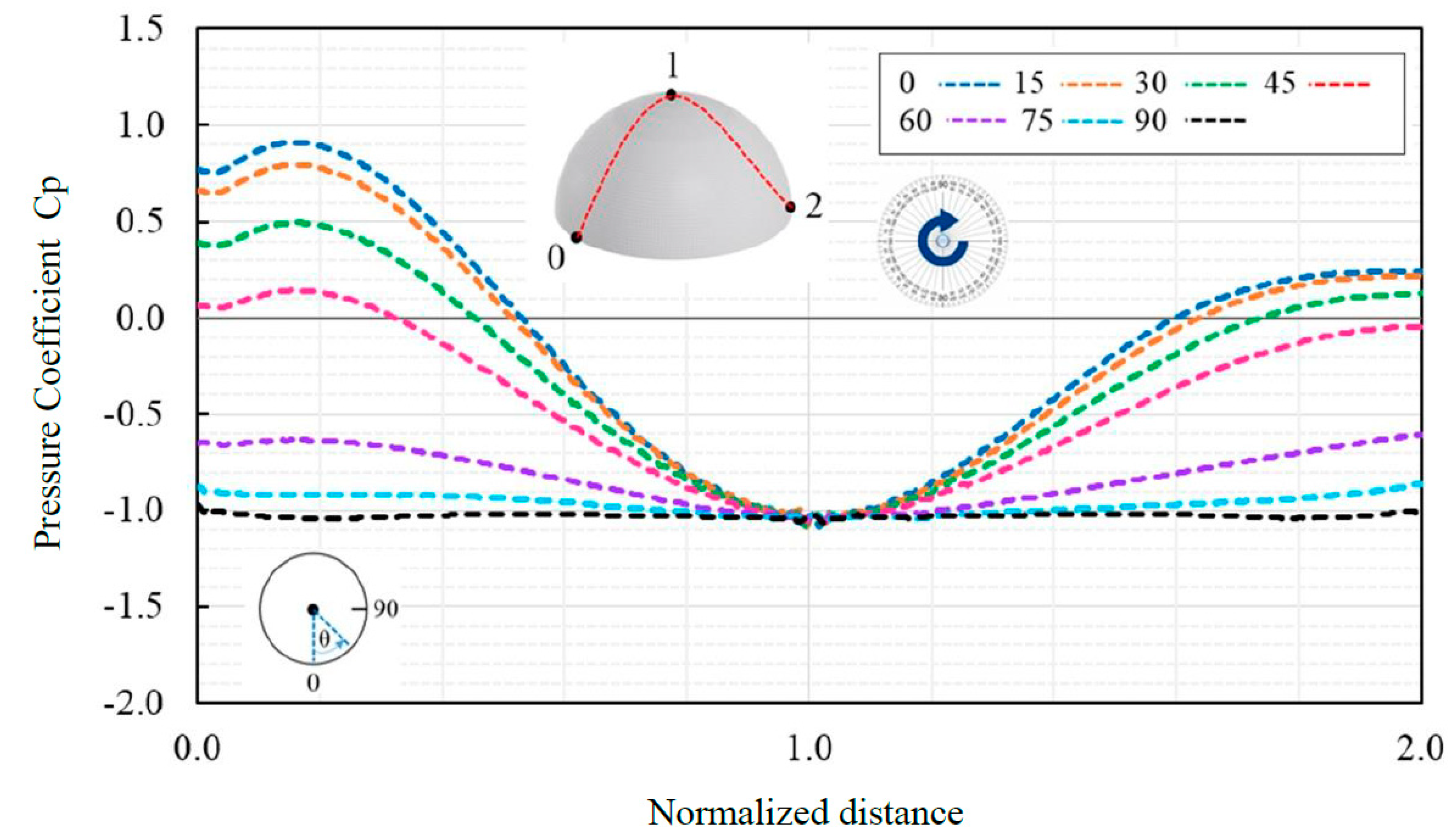
Figure 27.
Average of average wind pressure distribution on horizontal probe lines for hemisphere shape.
Figure 27.
Average of average wind pressure distribution on horizontal probe lines for hemisphere shape.

Figure 28.
Average Cp contour for hemisphere form.
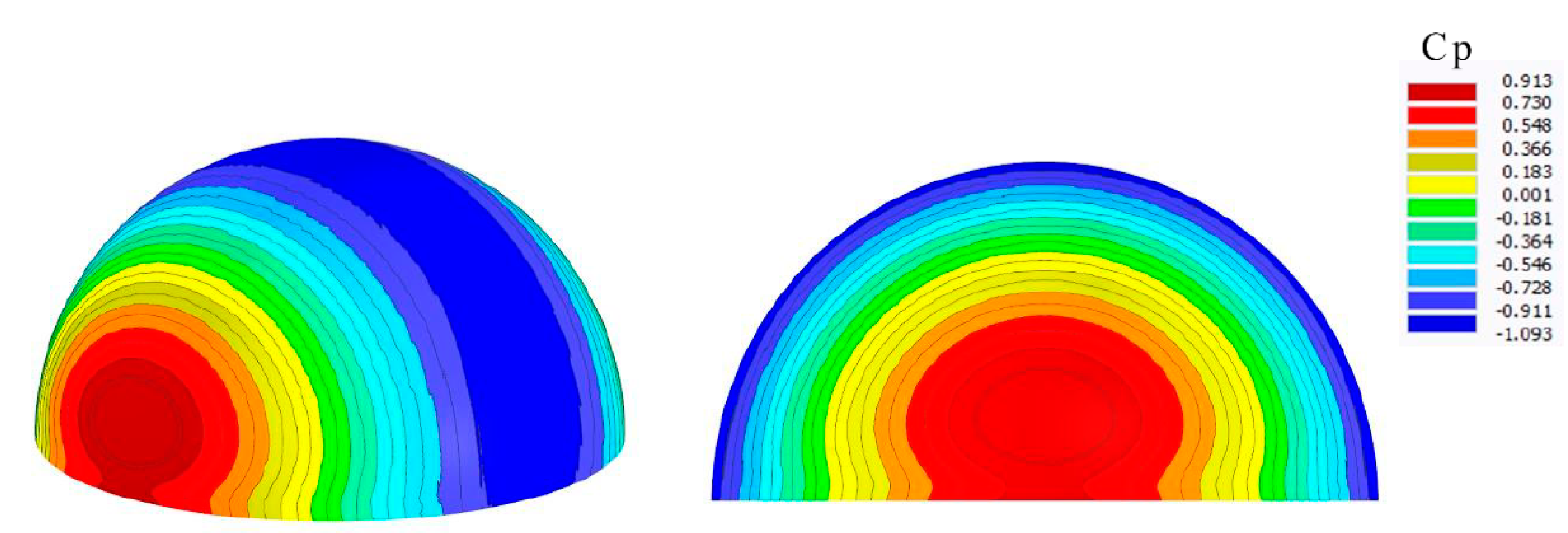

Table 1.
Model specifications.
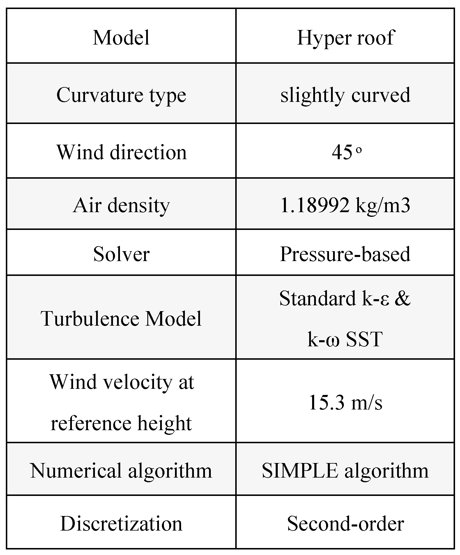
Table 2.
Drag forces and wind coefficient for conical form.

Table 3.
Drag forces and wind coefficient for tensile ridge valley form.
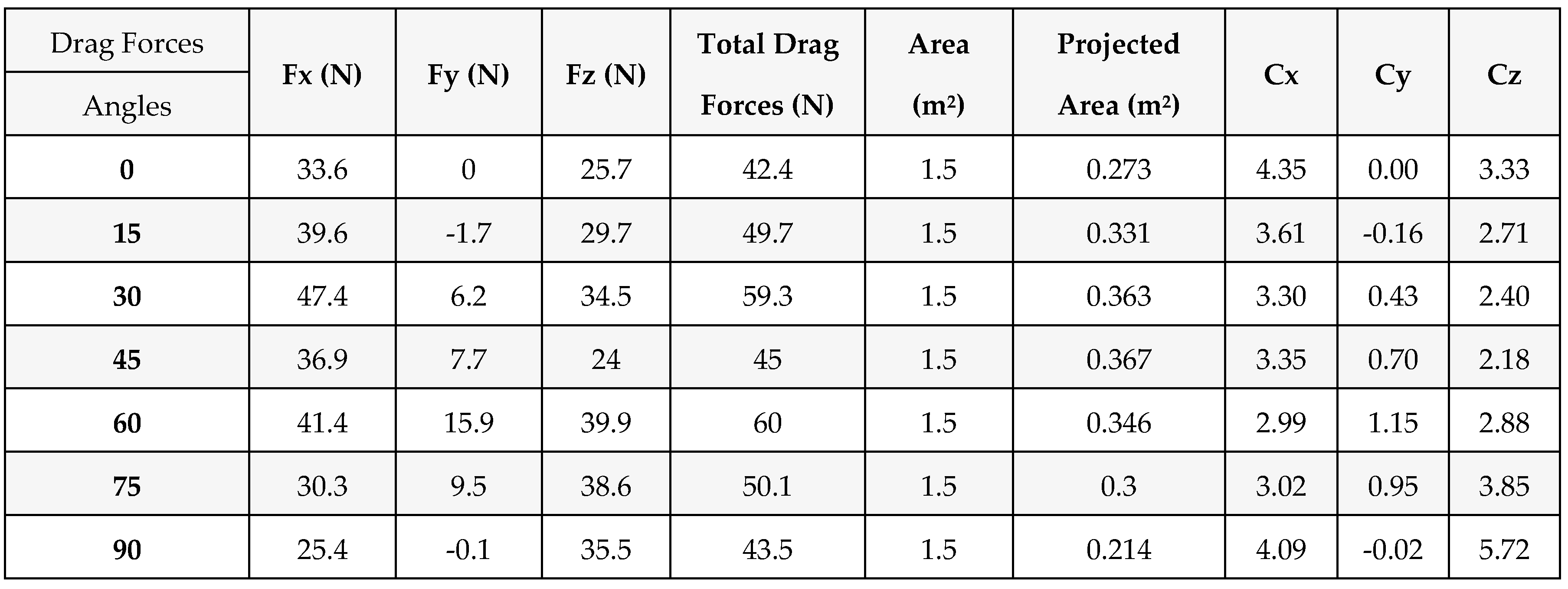
Table 4.
Drag forces and wind coefficient for Saddle form.

Table 5.
Drag forces and wind coefficient for cube form.
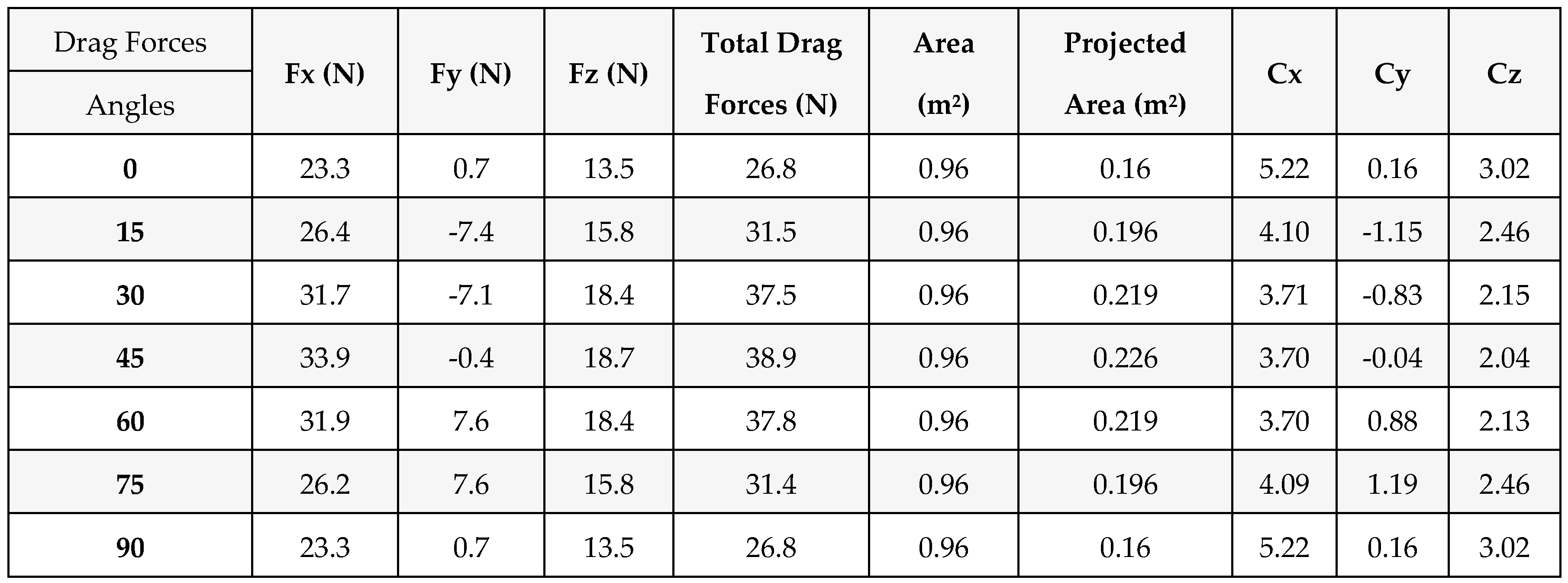
Table 6.
Drag forces and wind coefficient for the cylindrical shape.
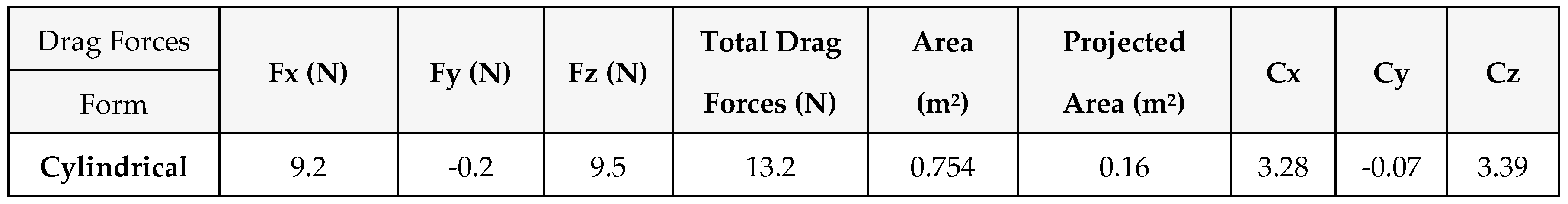
Table 7.
Drag forces and wind coefficient for Hemisphere form.
Disclaimer/Publisher’s Note: The statements, opinions and data contained in all publications are solely those of the individual author(s) and contributor(s) and not of MDPI and/or the editor(s). MDPI and/or the editor(s) disclaim responsibility for any injury to people or property resulting from any ideas, methods, instructions or products referred to in the content. |
© 2023 by the authors. Licensee MDPI, Basel, Switzerland. This article is an open access article distributed under the terms and conditions of the Creative Commons Attribution (CC BY) license (http://creativecommons.org/licenses/by/4.0/).
Copyright: This open access article is published under a Creative Commons CC BY 4.0 license, which permit the free download, distribution, and reuse, provided that the author and preprint are cited in any reuse.


