

Submitted:
09 October 2023
Posted:
11 October 2023
Read the latest preprint version here
Abstract
This article develops duality principles, a related convex dual formulation and primal dual formulations suitable for the local and global optimization of non-convex primal formulations for a large class of models in physics and engineering. The results are based on standard tools of functional analysis, calculus of variations and duality theory. In particular, we develop applications to a Ginzburg-Landau type equation. Other applications include primal dual variational formulations for a Burger's type equation and a Navier-Stokes system. We emphasize the novelty here is that the first dual variational formulation developed is convex for a primal formulation which is originally non-convex. Finally, we also highlight the primal dual variational formulations presented have a large region of convexity around any of their critical points.
Keywords:
convex dual variational formulations
; duality principles for non-convex local and global primal optimization
; Ginzburg-Landau type equation
MSC: 49N15
1. Introduction
In the first part of this article, we establish a duality principle and a related convex dual formulation suitable for the local optimization of a primal formulation for a large class of models in non-convex optimization. We highlight the first dual variational formulation presented is convex and such a feature may be very useful for a large class of similar models, in particularly for large systems in a three or higher dimensional context.
For such large systems the convexity obtained is relevant for an easier numerical computation, since in such a case of strict convexity, the standard Newton, Newton-type and other similar methods are always convergent.
We also emphasize the main duality principle is applied to the Ginzburg-Landau system in superconductivity in the absence of a magnetic field.
Other applications include primal dual formulations for a Burger’s type equation and a Navier-Stokes system.
For the duality principles, the results are based on the works of J.J. Telega and W.R. Bielski [1,2,3,4] and on a D.C. optimization approach developed in Toland [5].
About the other references, details on the Sobolev spaces involved are found in [6]. Related and more recent results on convex analysis and duality theory are addressed in [7,8,9,10,11]. In particular, the results in the present work are extensions and improvements of those results found in the recent book [12] and recent article [13], which by the way, are also based on the articles [1,2,3,4]. Similar models on the superconductivity physics may be found in [14,15].
Finally, we also emphasize in the last section we develop a duality principle for the quasi-convex relation of a general model in the vectorial calculus of variations.
Remark 1.
It is worth highlighting, we may generically denote
simply by
where denotes a concerning identity operator. Here it is also worth clarifying in general we will denote simply as
Other similar notations may be used along this text as their indicated meaning are sufficiently clear.
Finally, denotes the Laplace operator and for real constants and , the notation means that is much larger than
Now we present some basic definitions and statements.
Definition 1.
Let V be a Banach space. We define the topological dual space of V, denoted by , as the set of all continuous and linear functionals defined on V.
We assume may be represented through another Banach space denoted by and a bilinear form
More specifically, for each , we suppose there exists a unique such that
Moreover, we define the norm of f, denoted by
by
For an open, bounded and connected set and we recall that
More specifically, for each continuous and linear functional there exists a unique such that
Definition 2
(The first variation). Let V be a Banach space. Let be a functional.
We define the first variation of F at on the direction , denoted by as
if such a limit exists.
If there exists such that
we say that F is Gâteaux differentiable at u. Moreover, in such a case, is said to be the Gâteaux derivative of F at u.
We may also denote
Definition 3
(The second variation). Let V be a Banach space. Let be a functional.
We define the second variation of F at on the directions and , denoted by , as
if such a limit exists.
Definition 4
(Polar functional). Let V be a Banach space and let be a functional.
We define the polar functional of F, denoted by , by
Another important definition refers to the Legendre transform one and respective relevant propriety, which are summarized in the next theorem.
Theorem 1
(Legendre transform theorem). Let V be a Banach space and let be a twice continuously Fréchet differentiable functional.
Let . Assume there exists a unique such that
Suppose also
in a neighborhood of
Under such hypotheses, defining the Legendre tranform of F at by where
we have that
Remark 2.
Concerning such a last definition, observe that if F is convex on V, then the extremal condition
corresponds to globally maximize
on V, so that, in such a case,
Summarizing, if F is convex, under the hypotheses of the last theorem, the polar functional coincides with the Legendre transform of F on already denoted by , that is,
2. The primal variational formulation and the dual functional definitions
At this point we start to describe the primal and dual variational formulations.
Let be an open, bounded, connected set with a regular (Lipschitzian) boundary denoted by
Consider a functional where
Here , and
Moreover, and we denote
Define the functionals , by
and
At this point we assume a finite dimensional version for this concerning model. For example, we may define a new domain for the primal functional considering the projection of V on the space spanned by the first N (in general N=10, is enough) eigen-vectors of the Laplace operator, corresponding to the first N eigen-values. On this new not relabeled finite dimensional space V, since corresponds to a diagonal matrix, there exists such that
, where
for an appropriate real constant .
We define also by
and , by
and,
respectively.
Furthermore, we define
and by
Assuming (through a re-scaling, if necessary) and
by directly computing we may easily obtain that for such specified real constants, in convex in on
3. The main duality principle and a concerning convex dual formulation
Considering the statements and definitions presented in the previous section, we may prove the following theorem.
Theorem 2.
Let be such that
and be such that
Under such hypotheses, we have
and
Proof.
Observe that so that, since is convex in on , we obtain
Now we will show that
From
and
we have
and
Observe now that denoting
there exists such that
and
so that
Summarizing, we have got
Also, denoting
from
we have
so that
From such results, we may infer that
Moreover, from
we have
so that
From such last results we get
and thus
Furthermore, also from such last results and the Legendre transform properties, we have
so that
Finally, observe that from a concerning convexity,
Joining the pieces, we have got
The proof is complete.
□
4. A primal dual formulation for a local optimization of the primal one
In this section we develop a primal dual formulation corresponding to a non-convex primal formulation.
We start by describing the primal formulation.
Let be an open, bounded, connected set with a regular (Lipschitzian) boundary denoted by
For the primal formulation, consider a functional where
Here , and
Moreover, and we denote
Define the functional , by
We define also
for an appropriate real constant .
Furthermore, we define
for an appropriate real constant and
Now observe that denoting , we have
and
Denoting we have also that
In such a case, we obtain
Observe that at a critical point
and
From such results we may infer that
around any critical point.
With such results in mind, at this point and on assuming a related not relabeled finite dimensional model version, in a finite differences or finite elements context, we may prove the following theorem.
Theorem 3.
Let be such that
Under such hypotheses, we have
and there exists such that
Proof.
The proof that
and
may be done similarly as in the previous sections.
Observe that, as previously obtained, there exists such that
and
Since for a sufficiently large we have
from these last results and the standard Saddle point theorem, we have
The proof is complete. □
6. A numerical example
In order to illustrate the applicability of such results we have developed the following numerical example.
For , , and on we have solved the Ginzburg-Landau type equation
with
To obtain such numerical results, refereing to those previous ones of Section 3, we have used the following primal dual functional where
where
and,
Observe that a critical point of corresponds to a critical of the dual functional . From the convexity of , such a critical point corresponds a to a global optimal one for .
We have obtained results through finite differences combined with a MAT-LAB optimization tool. For an extensive approach on finite differences schemes, please see reference [16].
For the corresponding solution , please see Figure 1.
7. A primal dual variational formulation for a Burger’s type equation
In this section we develop a primal dual variational formulation for a Burger’s type equation.
Let be an open, bounded and connected set with a regular (Lipschitzian) boundary denoted by
Consider the Burger’s type equation in given by
where , and
At this point we define the functional where
Here Let
Observe that
and denoting we have
Therefore
Observe that at a critical point we have .
From this and (29) we may infer that is positive definite in a neighborhood of any critical point of J.
Thus, we may also conclude that the functional J has a large region of convexity around any of its critical points.
7.1. A numerical example concerning a Burger’s type equation
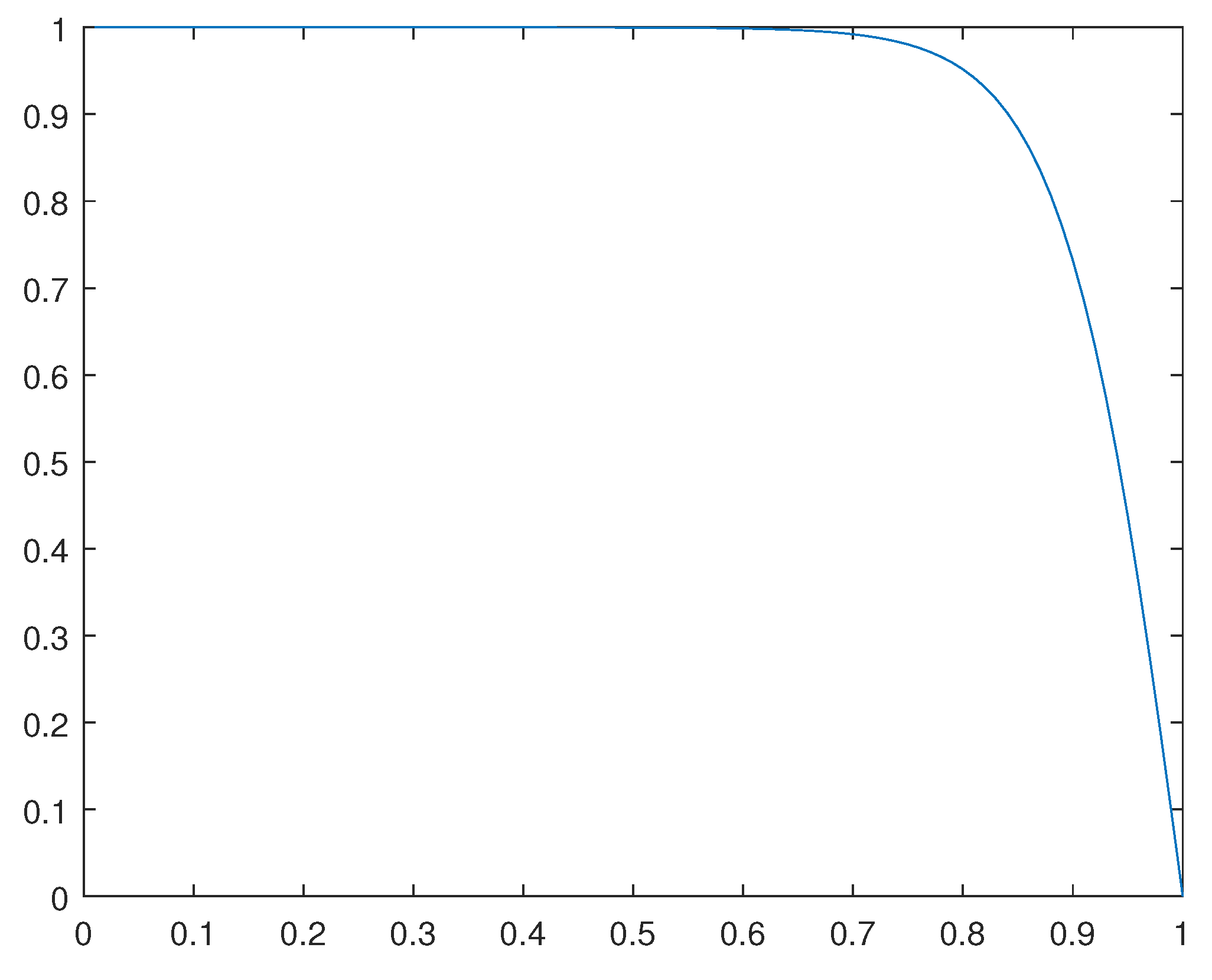
In this subsection we present numerical results related to a solution of the one-dimensional Burger’s equation
with the boundary conditions
For a first example we set and for the second one we set
To obtain the numerical results, we have used an adaptation with small changes of the primal dual variational formulation presented in the previous section.
For the solution for the case in which , please see Figure 2.
For the case in which , please see Figure 3.
Here we present the software in MAT-LAB through which we have obtained such numerical results.
We highlight to have searched for a critical point of the primal dual formulation previously presented with some small changes and adaptations. Indeed, we have developed a procedure similar to the matrix version of the generalized method of lines.
Here the software in a finite difference context, where A stands for :
**********
-
clear allm8=100;d=1/m8;K=5.0;A=0.5;for i=1:m8uo(i,1)=1.0;u1(i,1)=1.0;v3(i,1)=K*uo(i,1);end;k2=1;b14=1.0;while andk2=k2+1;k1=1;b12=1.0;while andk1=k1+1;i=1;m12=A*2+uo(i,1)*d+K*;m50(i)=A/m12;z(i)=1/m12*(A+v3(i,1)*+uo(i,1)*d);for i=2:m8-1m12=A*2-A*m50(i-1)+uo(i,1)*d-uo(i,1)*m50(i-1)*d+K*;m50(i)=A/m12;z(i)=1/m12*(v3(i,1)*+A*z(i-1)+uo(i,1)*z(i-1)*d);end;u(m8,1)=0.0;for i=1:m8-1u(m8-i,1)=m50(m8-i)*u(m8-i+1,1)+z(m8-i);end;b12=max(abs(u-uo));uo=u;end;b14=max(abs(u-u1));u1=u;for i=1:m8-1v3(i,1)=K*u(i,1);end;uo(50,1)end;for i=1:m8x(i)=i*d;end;plot(x,u)
************
10. Conclusion
In this article we have developed convex dual and primal dual variational formulations suitable for the local optimization of non-convex primal formulations.
It is worth highlighting, the results may be applied to a large class of models in physics and engineering.
We also emphasize the first duality principles here presented are applied to a Ginzburg-Landau type equation. In particular, we highlight the primal dual formulation presented in Section 5 which is suitable for the global optimization of a originally non-convex primal formulation.
Among the results, we have included primal dual variational formulations for a Burger’s type equation and for a time independent incompressible Navier-Stokes system. Concerning the Burger’s equation model, we have presented numerical examples and a related software in MAT-LAB.
Finally, in the last section, we have developed a new duality principle suitable for the relaxed quasi-convex primal formulation for a general model in a vectorial calculus of variations context.
In a future research, we intend to extend such results for some models of plates and shells and other models in the elasticity theory.
Data Availability Statement
Details on the software for numerical results available upon request.
Conflicts of Interest
The author declares no conflict of interest concerning this article.
References
- W.R. Bielski, A. Galka, J.J. Telega, The Complementary Energy Principle and Duality for Geometrically Nonlinear Elastic Shells. I. Simple case of moderate rotations around a tangent to the middle surface. Bulletin of the Polish Academy of Sciences, Technical Sciences, Vol. 38, No. 7-9, 1988.
- W.R. Bielski and J.J. Telega,A Contribution to Contact Problems for a Class of Solids and Structures, Arch. Mech., 37, 4-5, pp. 303-320, Warszawa 1985.
- J.J. Telega, On the complementary energy principle in non-linear elasticity. Part I: Von Karman plates and three dimensional solids, C.R. Acad. Sci. Paris, Serie II, 308, 1193-1198; Part II: Linear elastic solid and non-convex boundary condition. Minimax approach, ibid, pp. 1313-1317 (1989).
- A.Galka and J.J.Telega, Duality and the complementary energy principle for a class of geometrically non-linear structures. Part I. Five parameter shell model; Part II. Anomalous dual variational priciples for compressed elastic beams, Arch. Mech. 47 (1995) 677-698, 699-724.
- J.F. Toland, A duality principle for non-convex optimisation and the calculus of variations, Arch. Rat. Mech. Anal., 71, No. 1 (1979), 41-61. [CrossRef]
- R.A. Adams and J.F. Fournier, Sobolev Spaces, 2nd edn. (Elsevier, New York, 2003).
- F. Botelho, Functional Analysis and Applied Optimization in Banach Spaces, Springer Switzerland, 2014. [CrossRef]
- F.S. Botelho, Variational Convex Analysis, Ph.D. thesis, Virginia Tech, Blacksburg, VA -USA, (2009).
- F. Botelho, Topics on Functional Analysis, Calculus of Variations and Duality, Academic Publications, Sofia, (2011).
- F. Botelho, Existence of solution for the Ginzburg-Landau system, a related optimal control problem and its computation by the generalized method of lines, Applied Mathematics and Computation, 218, 11976-11989, (2012). [CrossRef]
- R.T. Rockafellar, Convex Analysis, Princeton Univ. Press, (1970).
- F.S. Botelho, Functional Analysis, Calculus of Variations and Numerical Methods in Physics and Engineering, CRC Taylor and Francis, Florida, 2020.
- F.S. Botelho, Dual Variational Formulations for a Large Class of Non-Convex Models in the Calculus of Variations, Mathematics 2023, 11(1), 63. [CrossRef]
- J.F. Annet, Superconductivity, Superfluids and Condensates, 2nd edn. ( Oxford Master Series in Condensed Matter Physics, Oxford University Press, Reprint, 2010).
- L.D. Landau and E.M. Lifschits, Course of Theoretical Physics, Vol. 5- Statistical Physics, part 1. (Butterworth-Heinemann, Elsevier, reprint 2008).
- J.C. Strikwerda, Finite Difference Schemes and Partial Differential Equations, SIAM, second edition (Philadelphia, 2004).
- P. Constantin and C. Foias, Navier-Stokes Equation, University of Chicago Press, Chicago, 1989.
- Makram Hamouda, Daozhi Han, Chang-Yeol Jung and Roger Temam, Boundary layers for the 3D primitive equations in a cube: the zero-mode, Journal of Applied Analysis and Computation, 8, No. 3, 2018, 873-889. [CrossRef]
- Andrea Giorgini, Alain Miranville and Roger Temam, Uniqueness and regularity for the Navier-Stokes-Cahn-Hilliard system, SIAM J. of Mathematical Analysis (SIMA), 51, 3, 2019, 2535-2574. [CrossRef]
- Ciprian Foias, Ricard M.S. Rosa and Roger M. Temam, Properties of stationary statistical solutions of the three-dimensional Navier-Stokes equations, J. of Dynamics and Differential Equations, Special issue in memory of George Sell, 31, 3, 2019, 1689-1741. [CrossRef]
- R. Temam, Navier-Stokes Equations, AMS Chelsea, reprint (2001).
- F.S. Botelho, Approximate Numerical Procedures for the Navier-Stokes System Through the Generalized Method of Lines. Preprints.org 2023, 2023020422. [CrossRef]
Figure 1.
Solution for the primal formulation.
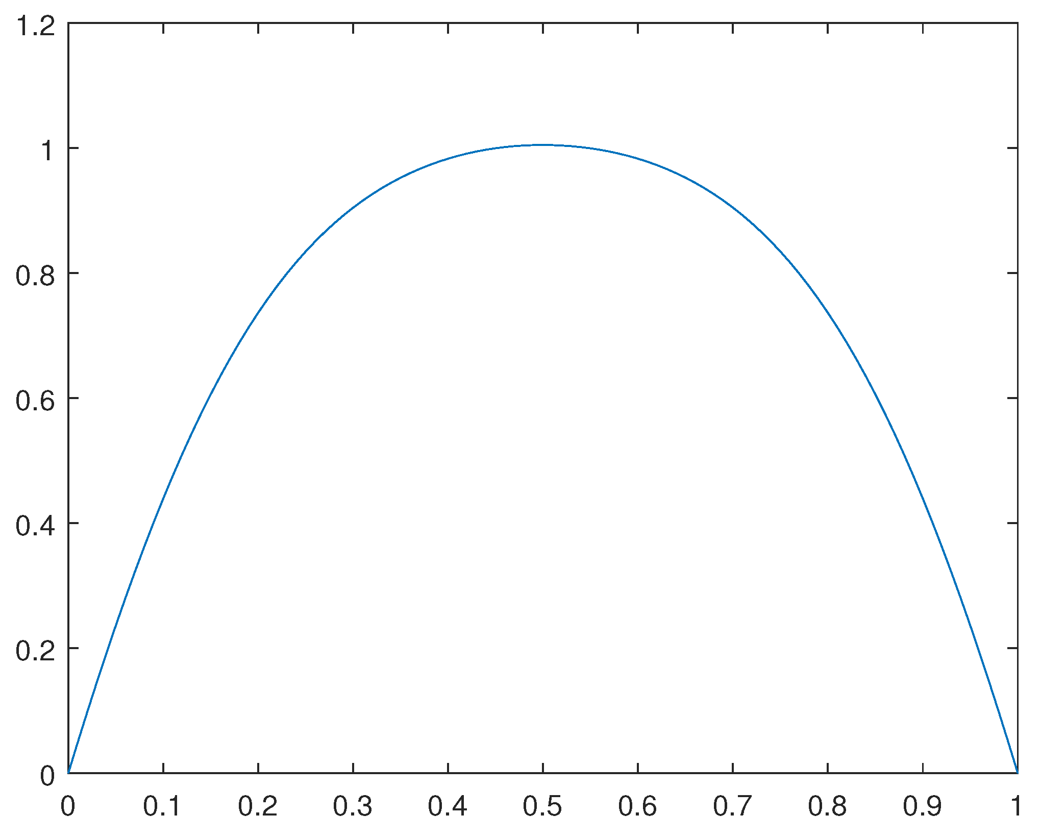
Figure 2.
Solution for a Burger’s type equation with .
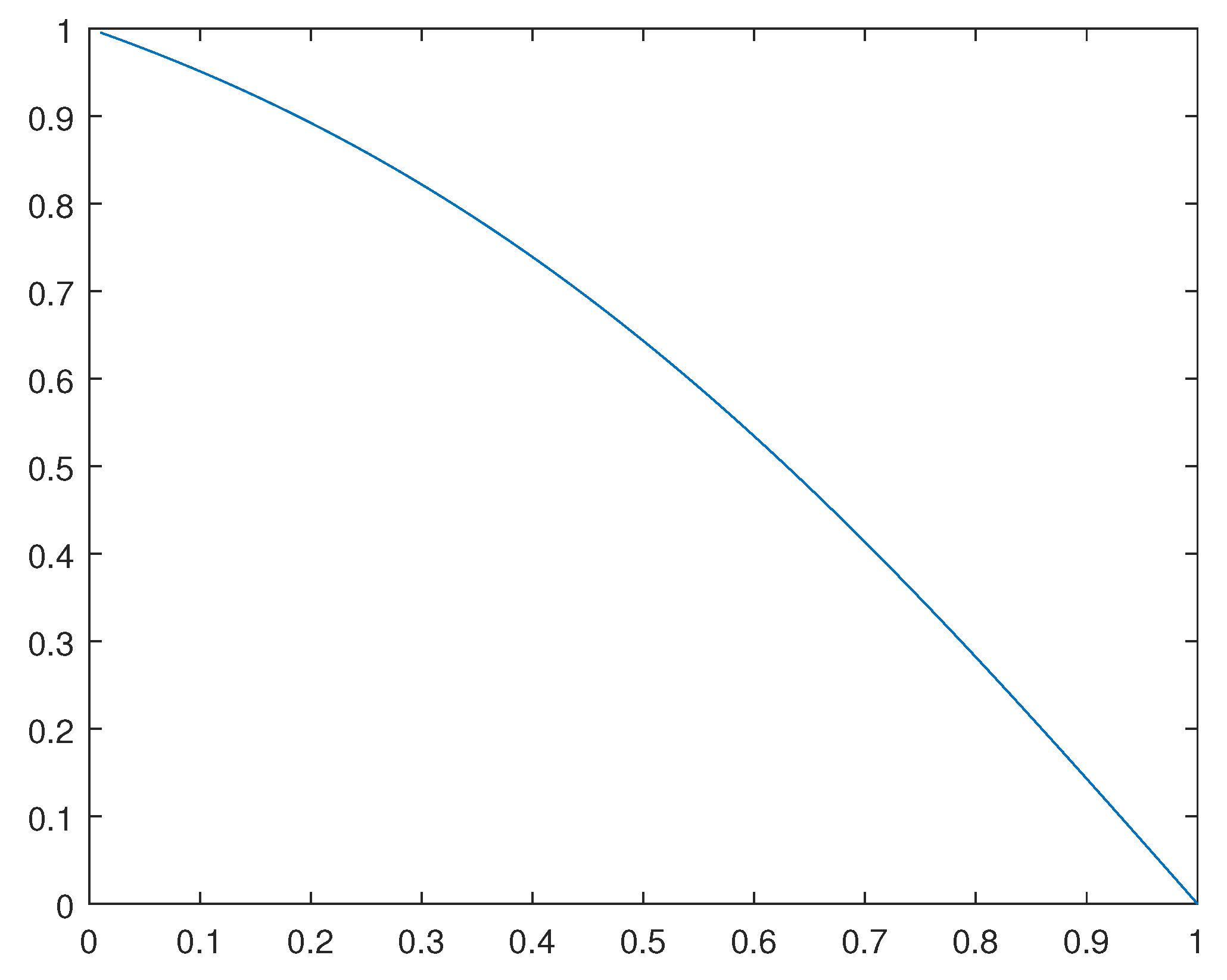
Figure 3.
Solution for a Burger’s type equation with .
Disclaimer/Publisher’s Note: The statements, opinions and data contained in all publications are solely those of the individual author(s) and contributor(s) and not of MDPI and/or the editor(s). MDPI and/or the editor(s) disclaim responsibility for any injury to people or property resulting from any ideas, methods, instructions or products referred to in the content. |
© 2023 by the authors. Licensee MDPI, Basel, Switzerland. This article is an open access article distributed under the terms and conditions of the Creative Commons Attribution (CC BY) license (http://creativecommons.org/licenses/by/4.0/).
Copyright: This open access article is published under a Creative Commons CC BY 4.0 license, which permit the free download, distribution, and reuse, provided that the author and preprint are cited in any reuse.