
Submitted:
17 November 2026
Posted:
18 November 2026
You are already at the latest version
Abstract
Small and medium-sized enterprises (SMEs) in the Peruvian metalworking sector plan production empirically, which leads to overstock, stockouts, and inefficient consumption of metal sheets. A systematic review of 97 recent studies showed that no previous solution integrates demand classification, per-product model selection, production deployment, and multi-company validation. This paper presents Predicast, a multi-tenant web platform with a ten-stage Machine Learning pipeline that combines Pareto-based product selection, ADI/CV² demand classification, feature engineering, and a Selective Algorithm Ensemble that chooses, for each product, among XGBoost, Random Forest, and Ridge through time-series cross-validation, translating 52-week forecasts into production recommendations. The system was validated with transactional data from 2021 to 2025 from four companies in the sector: the mean absolute percentage error (MAPE) was 10.79% at Electro SVM, 11.30% at Metal Perú, 11.65% at CMETAL, and 15.83% at Promelsa, the only distributor, for an overall MAPE of 12.39% and an R² of 0.77. User acceptance tests with 20 users yielded a SUS score of 75.8, and all 50 functional test cases passed. At the pilot company, a retrospective evaluation estimated that Predicast would have reduced overproduction costs by up to PEN 284,606 over 2021–2025, at an operating cost of about PEN 66 per month.
Keywords:
demand forecasting
; machine learning
; ADI/CV² classification
; MLOps
; metalworking SMEs
; XGBoost
1. Introduction
The metalworking sector is a strategic engine for Peru’s economic development: it contributes more than 9% of manufacturing GDP, comprises more than 74,000 companies, and generates around 350,000 formal jobs, according to the Ministry of Production [1]. Its products supply the construction, mining, and electrical industries across the board. Despite its importance, according to ComexPerú [2], organizations in the sector face logistical inefficiencies that consume on average 16% of their sales value, a figure that rises to 21.1% in smaller companies. In these organizations, raw material—mainly metal sheets and profiles—is the central input of production, and the adoption of digital innovation to use resources efficiently is a topic of recent interest in the metal industry [3]; therefore, any misalignment between what is manufactured and what is sold translates into tied-up capital and wasted inputs.
In practice, most metalworking SMEs plan their production manually, based on the plant manager’s experience and simple historical averages. As Gao and Sarvghadi [4] point out, under Make-to-Stock schemes the absence of quantitative estimates of future demand causes overstock in some products and stockouts in others, two symptoms of the same planning problem. The difficulty is compounded because demand for these products is erratic: orders are frequent, but their size varies considerably from week to week, a pattern that the Syntetos and Boylan framework identifies as one of the most difficult to forecast [5]. According to the studies by Zhang et al. [6] and Tjøstheim [7], classical statistical methods, such as ARIMA or exponential smoothing, struggle to capture nonlinear relationships between demand and its drivers.
The consequences of this way of planning are not limited to the company. Forecast errors propagate upstream in the supply chain and amplify order variability—the well-known bullwhip effect—which recent literature seeks to mitigate through better forecasting strategies and the use of artificial intelligence [8,9]. Demand forecasting for steel products and construction materials has also received recent attention, as in the studies by Sukolkit et al. [10] and Magableh et al. [11]. For an SME that buys sheets in batches and manufactures in advance, an inaccurate forecast implies both capital tied up in finished goods and poorly sized purchases of inputs.
From a technical standpoint, recent analyses of forecasting competitions and their application in retail show that tree ensembles, such as gradient boosting, combined with feature engineering, achieve outstanding results on real demand series [7,12,13], although no single approach is suitable for all products [14]. Transferring these advances to an SME also requires addressing data cleaning, model selection, and deployment in a system that the planner can use daily, with the engineering challenges this entails [15,16,17]. According to Lada et al. [18], Segarra-Blasco et al. [19], and Mandal et al. [20], SMEs face additional adoption barriers, such as a lack of digital skills, organizational readiness, and data.
As the systematic reviews by Vlachos and Reddy [21] and Babai et al. [22] show, the use of ML in the supply chain has become well established, and, according to Dey et al. [23], artificial intelligence can strengthen the resilience of manufacturing SMEs. However, its implementation faces organizational challenges: at an Italian manufacturer, a deep learning–based forecasting system required specific enablers and transformed the organization’s information processes [24], and the technological, organizational, and environmental barriers to adopting AI in forecasting reinforce one another [20]. In the case of SMEs, this gap is explained both by the adoption barriers already mentioned and by the absence of tools that integrate forecasting with the operational decisions that the planner makes each week.
Previous efforts address parts of the problem: ML models for demand forecasting in different sectors, specific methods for intermittent demand, MLOps architectures, and decision support systems (Section 2). In Latin America, recent studies published in high-impact journals analyze a single organization or rely on synthetic data [25,26], and the systematic review did not identify studies on Peruvian metalworking SMEs. The motivation for this work arises from a previous study by the authors at a manufacturer of metal electrical boxes, which observed systematic overproduction of between 6% and 7.6% in its critical products and validated a first prototype of the system; the open question was whether this approach could be generalized to other companies in the sector without manual adjustments.
Among the works closest to the present one, Kang et al. evaluated statistical, ML, and hybrid models in a Make-to-Stock manufacturing SME without extensive digital infrastructure [27]; Fries et al. analyzed how to integrate AI into the planning of three German metalworking SMEs [28]; da Silva et al. combined demand classification with ML and statistical models in a single company [25]; and the MLOps architectures reported in manufacturing correspond to large organizations, such as a steel plant [29]. None of them combines demand classification, per-product model selection, a system deployed in production, and evaluation with several companies from the same sector, and none addresses the context of Latin American metalworking SMEs.
The authors’ previous study also showed that the cost of the surplus raw material associated with the overproduction of seven products reached hundreds of thousands of soles (Section 4.12), which demonstrated that the problem had a concrete economic impact and not merely an operational one. At the same time, companies in the sector share features that favor a common solution: they manufacture catalog products—boxes, cable trays, rails, and accessories—from metal sheets, sell to customers in construction and the electrical industry, and record their warehouse movements in ERP systems with similar structures. Therefore, this work adopts the Design Science Research approach [30]: an artifact—a complete information system—is built and evaluated with real data from several companies to determine the extent to which the same design is applicable across the sector.
Objective. The objective of this work is to design, implement, and validate with real data from several companies a web-based demand forecasting and production planning support system for metalworking SMEs that automates the entire cycle, from loading ERP data to the weekly production recommendation. Its contributions are as follows:
- A systematic review of recent literature (2023–2026, Q1/Q2 journals) on ML-based demand forecasting, demand classification, MLOps, and decision support in SMEs, which identifies the gap that this work addresses.
- An automated ten-stage Machine Learning pipeline that integrates Pareto-based product selection, ADI/CV² classification, and a Selective Algorithm Ensemble (SAE) that selects, for each SKU, the best model among XGBoost, Random Forest, and Ridge Regression.
- A full-stack multi-tenant web system deployed in production on AWS, with containers, continuous integration, and automated deployment.
- An empirical validation with real transactional data from four companies in the Peruvian metalworking sector (18 SKUs, 2021–2025), which makes it possible to analyze the generalization capability of the approach within a single sector.
The remainder of the article is organized as follows: Section 2 presents the state of the art through a systematic review; Section 3 describes the proposal (architecture and pipeline); Section 4 details the validation protocol and results; Section 5 discusses the findings, their practical implications, and the threats to validity; and Section 6 presents the conclusions and future work.
2. Related Work
The state of the art was built through a systematic literature review that followed the guidelines of Kitchenham and Charters [31] and the PRISMA 2020 statement [32]. Four research questions guided it: which ML methods are used for demand forecasting and how they compare with statistical methods (RQ1); how demand is classified and how this conditions the choice of model (RQ2); which MLOps architectures are reported for deploying models in production (RQ3); and which decision support systems and ML adoption experiences are reported for SMEs (RQ4). Five search strings were applied to title and abstract in OpenAlex on 30 September 2026, limited to articles from 2023–2026 in Q1 or Q2 journals of the SCImago Journal Rank. Of the 1,498 records identified, 325 belonged to Q1/Q2 journals and 132 were assessed after screening and duplicate removal; 97 studies were included: 20 for RQ1, 27 for RQ2, 22 for RQ3, and 28 for RQ4.
The synthesis of the 97 included studies reveals four trends. First, tree ensembles—XGBoost in particular—are the most frequent Machine Learning approach for demand forecasting and usually outperform classical statistical models, but most evidence comes from retail, food, and spare parts, and the few studies with manufacturer data analyze a single organization. Second, the ADI/CV² classification remains the reference for characterizing demand, yet it is rarely used as a step prior to selecting ML models. Third, the MLOps literature is mostly conceptual or describes architectures for large organizations. Fourth, studies on SMEs stress that adoption requires affordable tools that work with limited data and that the planner can understand. Table 1 compares the works closest to this proposal.
None of these works combines, in a single solution, formal demand classification, automatic model selection per product, a system deployed in production, and validation with several companies of the same sector in an emerging market. Predicast contributes to closing this gap in three ways: it integrates the ADI/CV² classification as an explicit stage before per-SKU model selection; it operationalizes the pipeline in a web system deployed on low-cost infrastructure accessible to an SME; and it evaluates the same design with four companies of the Peruvian metalworking sector, which makes it possible to analyze its generalization within the sector.
3. Materials and Methods: the Predicast System
This work is framed within Design Science Research, in which the contribution is an artifact—in this case, an information system—that is designed to solve a relevant problem and is rigorously evaluated in its context of use [30]. The problem was identified at the pilot company; the artifact was designed and implemented as a web platform; and its evaluation was carried out with real data from four companies (Section 4). This section describes the software architecture, the data flow, and the Machine Learning pipeline.
3.1. Software Architecture
Predicast was implemented as a multi-tenant web application in which each company accesses its data, models, and forecasts in isolation. Figure 1 summarizes its three blocks: the continuous integration and deployment workflow, the production infrastructure, and the Machine Learning pipeline.
Presentation layer. The frontend is an application developed in Next.js 14 (Pages Router) and React, available on the system’s domain. All routes, except those for authentication, are protected by the NextAuth.js middleware, which delegates sign-in to Auth0 (Universal Login); user roles are carried as a token claim, and the administrator role enables user management through the Auth0 Management API with machine-to-machine (M2M) credentials. The interface is organized into four modules—Sales and Stock History, Finance, Production, and Administration—which cover historical analysis, sheet purchasing, production planning with operator targets, and user administration.
Service layer. The system logic is distributed across three services. (i) The Next.js API routes handle the business logic of the dashboards—historical series, sheet GAP, production plan, finance, operator assignment, and data upload—based on the pipeline outputs. (ii) A FastAPI REST API (Python 3.11), with Pydantic schemas and JWT authentication, exposes the forecasting (`/forecast/predict`), recommendation (`/forecast/recommend`), and pipeline execution (`/forecast/pipeline/run`) services, in addition to a health check endpoint. (iii) The Pipeline Service, implemented in Flask, exposes the `/run`, `/status`, `/logs`, `/cancel`, and `/health` endpoints; upon receiving an execution request, it launches the ten stages in a separate thread, logs the start and end of each stage, and checks between stages whether the user has requested cancellation, which allows the process to be interrupted safely.
Persistence layer. PostgreSQL 16 stores the platform entities (companies or tenants, users, and predictions), and Redis 7 is deployed as a cache. Operational data are shared among services through a file volume that contains the ERP exports, the exploratory analysis outputs, the optimization reports, and the 52-week forecasts; the finance configuration, the operator catalog, and the weekly assignments are stored as JSON documents in that same volume. This file-based design simplifies deployment on a single instance and makes the outputs of each run traceable.
Infrastructure and security. The five services—PostgreSQL, Redis, backend, frontend, and pipeline—are defined in Docker Compose with health checks and explicit dependencies, and run on an AWS EC2 t3.micro instance (us-east-1). Nginx acts as a reverse proxy, redirects HTTP traffic to HTTPS, and terminates TLS 1.2/1.3. The choice of a low-cost instance responds to the resource constraints typical of SMEs described by Mandal et al. [20] and Venanzi et al. [35].
Continuous integration and deployment. The GitHub Actions workflow consists of four chained jobs: (1) static analysis with ruff; (2) automated testing with pytest (15 cases covering the pipeline stages, feature selection, and the forecasting API), with a minimum coverage threshold of 25% on the pipeline scripts; (3) building of the backend, frontend, and pipeline images with docker buildx and their publication to Amazon ECR, tagged with the commit identifier; and (4) deployment to the EC2 instance via SSH, restricted to the main branch and the production environment. This workflow applies the principles of automation, versioning, and reproducibility proposed for MLOps [15,36] and reduces the risks associated with manual model deployment [16,17]. Unlike architectures aimed at large organizations [29,37], the solution is limited to open-source components on a single instance, in line with the open architecture of Burgueño-Romero et al. [38].
3.2. Data Flow
The usage cycle follows five steps. (1) The user authenticates through Auth0. (2) From the Production module, the user uploads the movement export from their ERP (`Movimientos_MayorAuxiliar_AAAA.csv`, semicolon-separated); the ingestion route verifies the file name and the presence of the date, inflow, and outflow columns, saves it in the new data directory, and records the upload in a log. (3) When “Run pipeline” is clicked, the frontend sends the request to the Pipeline Service and periodically queries its status and logs; the interface estimates a duration of 60 to 90 minutes for the full pipeline. (4) The pipeline writes to the shared volume the exploratory analysis results, the optimization report with the winning algorithm and the metrics for each SKU, and the 52-week forecasts with their confidence bands. (5) The frontend API routes read these files to build the dashboards, the production plan, and the financial analyses.
3.3. Input Data and Preprocessing
The data come from the companies’ ERP systems, exported in transactional format (warehouse movements, one or more files per year). Each record contains the variables summarized in Table 2, with daily granularity. At the pilot company, the period from January 2021 to May 2025 comprises 53,701 movements, of which 29,339 correspond to sales; the catalog includes 2,924 codes, 1,518 of them with sales, distributed across three warehouses and two channels (online and in-store).
Domain cleaning rules. Before any analysis, transfers between warehouses and delivery notes whose inflows and outflows offset each other are excluded, as they represent internal movements rather than demand. Next, for each SKU, outflow and inflow values above the 99th percentile are capped at that percentile, which corrects data-entry errors without removing legitimate large orders from the business channel.
Outlier treatment. The interquartile range (IQR) method is applied to TOP20 sales independently for each SKU, a criterion that is robust to extreme values, defined as
with the outlier detection limits given by
Observations outside these limits are replaced by the median of the SKU’s sales, rather than removed, to preserve the temporal continuity of the series.
Imputation. After weekly aggregation, weeks without transactions for a SKU are reconstructed using the complete ISO calendar, and their demand is linearly interpolated, bounded to non-negative values.
3.4. Product Selection and Demand Classification
Since each company handles hundreds of items, the pipeline ranks SKUs by sales volume, retains the 20 with the highest turnover (stage 03), and applies to them the Pareto principle, the basis of ABC inventory classification [39], to retain the subset that accounts for most of the volume (stage 05A). At the pilot company, with data from 2021 to 2025, six SKUs accounted for 78.1% of TOP20 sales. In the multi-company validation, this procedure yielded between 4 and 6 critical SKUs per company, 18 in total (Section 4).
The classification of Syntetos, Boylan, and Croston [5] (stage 05B) is applied to the selected SKUs, based on two metrics:
where N is the total number of periods, n the number of periods with positive demand, σy the standard deviation, and ȳ the mean of demand in the periods with positive demand. With the thresholds ADI = 1.32 and CV² = 0.49, demand is classified as smooth, erratic, intermittent, or lumpy [5]. The pipeline computes both metrics on the weekly series of each critical SKU and assigns series with ADI < 1.32 to the local modeling group—an independent model per SKU, trained on its own historical features—while reserving intermittent series for a joint global model. Specific methods exist for intermittent series, such as Croston’s method and its variants [40] or those based on temporal aggregation [41,42]; as shown in Section 4.5, all evaluated SKUs exhibited demand in every week, so only the local strategy was applied in this study.
3.5. Feature Engineering and Selection
The daily transactions of the critical SKUs were aggregated into ISO weeks (with Monday as the first day). For each week, in addition to total sales, the number of transactions; the mean, minimum, and maximum sale; the intra-week standard deviation; and the mode of the customer, channel, and dispatch point were calculated. From these, features of seven types were generated: calendar and Fourier, lags, moving averages and volatility, trends, intermittency and anomaly indicators, behavioral ratios, and encoded contextual features.
Calendar and Fourier features. These capture the seasonality and cyclicality of the series (Table 3). Fourier encoding represents time continuously and avoids the discontinuity of ordinal variables; According to the study by Ye et al. [43], Fourier terms are useful to model demand seasonality in retail.
Demand lags. These constitute the historical memory of the process:
Short-term lags (k = 1, 2, 3, 4) capture immediate autocorrelation; k = 13 represents the quarterly pattern and k = 52 the annual seasonality, a common practice in weekly sales forecasting with tree ensembles [12,44].
Moving averages and volatility. These are calculated as
with span ∈ {4, 13}. As described by Borucka [45], exponential smoothing assigns greater weight to recent observations and acts as a smoothed trend indicator.
Behavioral ratios. These are constructed from the intra-week statistics:
- Ratio_Transacciones: number of transactions in the week relative to its average over the last four weeks.
- Ratio_Min_Max: ratio between the minimum and maximum sale of the week; values close to 0 indicate a one-off large order.
- Variabilidad_Intra: coefficient of variation of the week’s transactions; it distinguishes many small customers from a few large customers.
Trends and additional indicators. These include the relative deviations from the 4- and 8-week moving averages, a linear time trend, the year-over-year ratio relative to the same week of the previous year (bounded to [0, 5]), the number of weeks elapsed since the last sale [40], and an anomaly indicator that flags weeks whose demand falls more than 30% below its 4-week moving average.
Contextual features. The predominant customer, sales channel, and dispatch point of each week, as well as the quarter, are encoded as binary variables.
Feature selection. In stage 07, the Pearson correlation of each feature with demand and the variance inflation factor (VIF) were calculated to detect multicollinearity. Based on these analyses, three sets are constructed (Table 4): the conservative and intermediate sets exclude features with VIF > 10 and retain only the 2- and 13-week moving averages, whereas the aggressive set keeps all features without problematic multicollinearity. In the evaluated version, the three sets are exported as analysis artifacts, and hyperparameter optimization is performed on the full feature set, leaving implicit selection to the algorithm through regularization and feature importance. The relevance of this stage is consistent with Giannopoulos et al. [46] and Nathan et al. [47], who found that feature engineering matters more than model complexity.
3.6. Selective Algorithm Ensemble (SAE)
Instead of applying a single global model, the SAE has three algorithm families compete for each SKU: Ridge Regression [48] as a regularized linear baseline, Random Forest [49] as a bagging ensemble, and XGBoost [50] as a boosting ensemble with L1/L2 regularization. The models were implemented with scikit-learn and XGBoost 2.0.3, with a fixed random seed to ensure reproducibility. Hyperparameters were optimized through grid search (`GridSearchCV`), a strategy also used in retail sales forecasting [51], with time-series cross-validation (Section 4.2) and R² as the criterion, over the following spaces:
- XGBoost: n_estimators ∈ {100, 200, 300}, max_depth ∈ {3, 4, 5, 6}, learning_rate ∈ {0.05, 0.1}, subsample = 0.8, colsample_bytree = 0.8, min_child_weight = 3.
- Random Forest: n_estimators ∈ {100, 200}, max_depth ∈ {5, 8}, min_samples_split ∈ {5, 8}, min_samples_leaf = 2.
- Ridge: alpha ∈ {1.0, 10.0, 100.0}.
Algorithm 1 formalizes the procedure. For each SKU, the algorithm with the highest mean R² across the validation folds is selected as the winner; for that model, the MAE, RMSE, and MAPE are recalculated using the same temporal partition. The final model is retrained on the last 104 weeks (two years) to reflect the recent demand level and reduce level-drift bias in recursive forecasting.
| Algorithm 1. Selective Algorithm Ensemble (SAE) per SKU. |
| 1: Input: weekly series with features (Xs, ys) for each critical SKU s; families = {Ridge, RF, XGBoost} with their grids Θm 2: Output: winning model fs and validation metrics per SKU 3: for each SKU s do 4: split (Xs, ys) into k = 5 consecutive temporal folds (TimeSeriesSplit) 5: for each family m ∈ do 6: for each combination θ ∈ Θm do 7: train on folds 1…i and validate on fold i + 1, for each fold i 8: R²(m, θ) ← mean validation R² across the five folds 9: θ*m ← arg maxθ R²(m, θ) 10: m* ← arg maxm R²(m, θ*m) 11: fs ← retrain m* with θ* on the last 104 weeks 12: record validation MAPE, RMSE, MAE, and R² of m* 13: return {fs} and their metrics |
3.7. Recursive Forecasting and Planning Logic
With the winning model, a 52-week forecast is generated using the recursive strategy, one of the two common multi-step strategies alongside the direct strategy [52]:
where ŷ is the predicted value, t the current time, h the horizon, and f(·) the learned function. The strategy trains a single one-step model and applies it iteratively for h = 1, …, 52: lags and moving averages are updated with the previous predictions, and calendar features are computed from the actual date of each future week. According to Sarıcıoğlu et al. [8], the choice between one-step and multi-step strategies also affects error propagation along the chain. Negative predictions are truncated at zero. A seasonal index by week of the year, bounded to the range [0.2, 4.0], is applied to the base prediction; to prevent seasonality from being amplified cumulatively, the lag buffer is fed with the base prediction rather than the adjusted one:
The 95% confidence bands are obtained by propagating the standard error with the square root of the horizon, under the assumption of independent errors:
The forecasts feed a decision-support module that computes the production plan per SKU for the 52 weeks of the horizon (Algorithm 2). The safety stock equals w weeks of mean forecast demand, with w = 2 by default; production is recommended only when projected stock would fall below that level, in the quantity required to restore it. Before planning, each weekly forecast is capped at five times the historical median of sales, which prevents an atypical peak from triggering excessive production. From the recommended production and the sheet consumption per unit of each product, the system calculates the required sheets and the sheet GAP, which expresses the accumulated overstock in units of raw material.
| Algorithm 2. Weekly production recommendation per SKU (planning module). |
| 1: Input: forecast ŷ1…52; current stock I0; historical median of weekly sales m; safety weeks w ∈ [0.5, 12] (default 2) 2: Output: weekly schedule of demand, production, and stock 3: ŷh ← min(ŷh, max(5m, 100)) for all h ▹ cap for atypical peaks 4: SS ← w · mean(ŷ1…52) ▹ safety stock 5: I ← I0 6: for h = 1…52 do 7: if I − ŷh < SS then Ph ← max(0, ŷh + SS − I) ▹ trigger 8: else Ph ← 0 9: flag the week as urgent if I − ŷh < 0 10: I ← I + Ph − ŷh 11: return {ŷh, Ph, I}; the required sheets are obtained from Ph and the per-unit consumption |
4. Validation and Results
4.1. Experimental Design: Companies and Data
Validation was performed with transactional data from four companies in the Peruvian metalworking sector—Electro SVM, Metal Perú, Promelsa, and CMETAL—provided by the companies themselves as warehouse movement exports and covering the period 2021–2025. The same automated pipeline described in Section 3 was applied to each company, with no company-specific manual adjustments. Corporación Electro SVM, a manufacturer of metal electrical boxes, is the pilot company of the previous study.
Table 5 characterizes the companies based on their public information (corporate websites), compiled and cross-checked with NotebookLM. Three of them manufacture metal products for electrical installations—boxes, condulets, cable trays, raceways, and support hardware—and one, Promelsa, is mainly engaged in the distribution of electrical materials, which makes it possible to contrast the approach on manufacturers and on a distributor. The descriptions of the SKUs evaluated in each dataset are consistent with these product lines: condulets and pull boxes at CMETAL, octagonal and rectangular boxes at Electro SVM, NEMA trays and fittings at Metal Perú, and EMT conduit and raceways at Promelsa.
Table 6 summarizes the datasets. Electro SVM provides the largest dataset, with 2,924 codes and three warehouses; for the other three companies, the data supplied correspond to their seven main products, with between 12,900 and 15,800 sales over five years. The Pareto analysis retained between 4 and 6 critical SKUs per company, which account for between 69.7% and 78.5% of TOP20 sales; in total, 18 SKUs were evaluated.

Table 6.
Characteristics of the datasets and critical SKUs selected by the pipeline.
| Company | Records | Sales | Codes | Period | Critical SKUs | % TOP20 sales |
|---|---|---|---|---|---|---|
| CMETAL | 16,657 | 12,948 | 7 | 2021-01 a 2026-01 | 4 | 69.7% |
| Electro SVM | 65,031 | 35,032 | 2,924 | 2021-01 a 2025-12 | 6 | 78.1% |
| Metal Perú | 16,712 | 12,963 | 7 | 2021-01 a 2026-01 | 4 | 78.5% |
| Promelsa | 20,414 | 15,822 | 7 | 2021-01 a 2026-01 | 4 | 78.3% |
Table 7.
Critical SKUs evaluated per company.
| Company | No. of SKUs | SKUs evaluated |
|---|---|---|
| CMETAL Condulet Perú | 4 | CAP 010, CDL 001, CDL 002, CDL 003 |
| Electro SVM | 6 | CEO 001, CEO 006, CER 001, CER 004, CER 005, CER 008 |
| Metal Perú S.A.C. | 4 | BNV 001, CPM 001, CPM 002, UNM 001 |
| Promelsa S.R.L. | 4 | CAJ 020, CAN 001, TCD 001, TCD 002 |
| Total | 18 |
4.2. Execution Environment and Reproducibility
All results in this section were obtained by running stages 03 to 09 of the pipeline in the project repository (version 92256ce) on the data of the four companies, in an environment isolated from the deployed system: Python 3 with pandas 3.0.2, scikit-learn 1.8.0, XGBoost 2.0.3, and statsmodels 0.15, on 2 vCPUs and 7 GB of memory, with a fixed random seed. Hyperparameter optimization and validation of one SKU took 48 s on average, and the full evaluation of the 18 SKUs took about 14 minutes. This run reproduces a previous validation performed by the authors with the same code: the winning algorithm matches for all 18 SKUs, and the mean absolute difference in MAPE is 0.21 points (maximum 1.04), attributable to library versions.
4.3. Time-Series Cross-Validation
To prevent the evaluation from using future observations, time-series cross-validation with an expanding window (TimeSeriesSplit) was used, whose finite-sample behavior has recently been analyzed [53], and which addresses the importance of data partitioning highlighted in the ML forecasting literature [46]. The number of folds is set to min(5, max(2, ⌊n/4⌋)), which, with the 259 to 263 weeks available per SKU, equals k = 5. In fold i, the model is trained on folds 1 to i and validated on fold i + 1; the metrics are computed on each validation fold and averaged.
4.4. Evaluation Metrics
Four complementary metrics, commonly used in the reviewed studies [33,54], are reported, where yt is the actual demand, ŷt the forecast demand, ȳ the mean of the actual demand, and n the number of validation weeks:
MAPE expresses the error in relative terms and allows SKUs and companies of different scales to be compared; in the implementation, it is computed only over weeks with positive demand, and each percentage error is capped at 200%. RMSE and MAE measure the error in product units, and R² indicates the proportion of variability explained by the model; a negative R² means that the model is worse than predicting the mean of the validation fold. As a reference, three naïve methods were evaluated on the same folds: the value of the previous week (t − 1), that of the same week of the previous year (t − 52), and the moving average of the four previous weeks.
4.5. Demand Classification of the Evaluated SKUs
All 18 SKUs had demand in every week (ADI = 1.00) and CV² values of the weekly series between 0.14 and 0.22 (Table 8). According to the Syntetos and Boylan thresholds, this pattern corresponds to smooth, non-erratic demand: weekly aggregation dampens the variability of individual orders, whose squared coefficient of variation is close to 1 (for example, between 0.90 and 0.99 for the SKUs of the pilot company). The pipeline groups series with ADI < 1.32 into the local modeling strategy—labeling them as “hybrid erratic” when CV² < 0.49—so the 18 SKUs were modeled with an independent model per product. The highest CV² values correspond to Promelsa, the company with the largest error (Section 4.9).
4.6. Results by Company
Table 9 summarizes the metrics by company, sorted from lowest to highest MAPE, and Figure 2(a) presents them graphically. The average MAPE of the four companies was 12.39% (standard deviation of 2.32 points), and the average R² was 0.77. Electro SVM achieved the lowest MAPE (10.79%) and the highest R² (0.8528), whereas Promelsa showed the weakest performance (MAPE of 15.83% and R² of 0.5943).
The three manufacturing companies are concentrated in a narrow MAPE band between 10.79% and 11.65% (mean of 11.25% and standard deviation of 0.43 points), with an average R² of 0.830; XGBoost was the dominant algorithm in all of them. Promelsa shows a larger relative error and the highest RMSE in the sample (923.58 units).
4.7. Comparison Between Algorithms
Figure 3 shows the cross-validation R² of the three algorithms for each SKU, and Table 10 summarizes the selection frequency. XGBoost won in 12 of the 18 SKUs (66.7%), Ridge in 5 (27.8%), and Random Forest in 1 (5.6%). Averaged over the 18 SKUs, R² was 0.756 for XGBoost, 0.705 for Random Forest, and 0.390 for Ridge. Ridge shows the greatest dispersion: it is the best model for five SKUs—CEO 001 and CER 005 of Electro SVM and CAN 001, TCD 001, and TCD 002 of Promelsa—but obtains a negative R² for 3 SKUs. Random Forest almost always falls below XGBoost and wins only for CAJ 020 of Promelsa. This pattern supports the decision to select the model per SKU rather than imposing a single algorithm, as recommended by Ma et al. [14] and Sfiris and Koulouriotis [55].
Table 11 details, for each SKU, the R² of the three algorithms and the metrics of the winner. At the SKU level, MAPE ranged from 9.06% (CER 004, Electro SVM) to 17.17% (TCD 001, Promelsa), with a median of 11.63%; 15 of the 18 SKUs (83.3%) obtained a MAPE equal to or below 15%.
4.8. Comparison with Baseline Methods
Figure 4 compares the MAPE of the winning model with the three naïve methods evaluated on the same folds. In the pipeline configuration, the selected model obtained a mean MAPE of 12.21%, compared with 35.13% for the 4-week moving average, 44.90% for the naïve method (t − 1), and 43.07% for the seasonal naïve method (t − 52), and it outperformed all three methods on all 18 SKUs. As discussed in Section 4.10, this advantage depends on the features built with information from the forecast week.
4.9. Generalization Within the Sector
The correlation between MAPE and R² was -0.88 at the SKU level and -0.99 at the company level (Figure 2(b)). The 3 SKUs with MAPE above 15% belong exclusively to Promelsa, whereas the 14 SKUs of the three manufacturing companies remained below that threshold. Consequently, the coefficient of variation of MAPE across companies, 18.7%, drops to 3.8% when Promelsa is excluded. With only four companies, the company-level correlation should be read as descriptive.
The characteristics of the company offer a plausible explanation for this case. Promelsa is the only distributor in the sample (Table 5), with a broad portfolio of electrical materials whose demand depends on third parties; it has the highest CV² values and is the only company where linear models dominated. Its demand could be more influenced by project orders or by external factors not included in the model, which suggests that the approach is better suited to manufacturers of catalog products.
4.10. Sensitivity Analysis: Forecast-Week Features
A review of the feature importance of the winning model showed that, for all 18 SKUs, the most influential feature belongs to the group of features computed with information from the very week being forecast: the deviations from the moving averages (`Trend_vs_MA4` and `Trend_vs_MA8`), which use that week’s sales in their numerator; the anomaly indicator; the intra-week ratios (transactions, minimum/maximum, and variability); the counters of weeks with sales; and the modes of customer, channel, and dispatch point. In cross-validation, these features are available, but in a real forecast they are not known until the week ends, which constitutes target information leakage, a methodological error documented in numerous ML applications and also in time-series forecasting [56,57].
To quantify its effect, the evaluation was repeated with two additional configurations, keeping the data, temporal folds, and hyperparameter grids identical: (i) excluding these features and (ii) retaining them but lagged by one week, so that they use only information available at forecast time. Table 12 summarizes the results. In the corrected configuration, the mean MAPE increased from 12.21% to 34.59%, and the mean R² went from 0.78 to -0.26; the selected model outperformed the 4-week moving average on 10 of the 18 SKUs, and Random Forest became the winner for all of them. In other words, with information strictly available at forecast time, the performance of the models is comparable to that of the moving average (35.13%), and the advantage observed in the pipeline configuration is mainly explained by these features.
This result does not invalidate the system, but it does delimit the scope of the metrics in Sections 4.6 to 4.9: they measure the ability of the models to estimate a week’s demand when contemporaneous information is available, not their ability to forecast in advance. Correcting the computation of these features in the pipeline, together with the evaluation of additional methods, is part of future work (Section 6).
4.11. Behavior of the 52-Week Forecast
Figure 5 shows the recursive forecast for the SKU with the lowest error (CER 004, Electro SVM) and for the one with the highest error (TCD 001, Promelsa). In both cases, the forecast level falls below the recent historical level: across the 18 SKUs, the median ratio between the mean forecast demand and the mean demand of the last 52 weeks was 0.33, and for one SKU with a Ridge model (TCD 002, Promelsa), the recursion produced divergent values. This behavior is consistent with the previous finding: during recursion, the forecast-week features cannot be recomputed and retain the value of the last observed week. In the planning module, the cap of five times the historical median contains the divergent values but does not correct the underestimation of the level; therefore, production recommendations should be interpreted with caution until the correction is applied.
4.12. Economic Impact on the Pilot Company
The exploratory analysis of the relationship between production and sales at Electro SVM, generated by stages 01 and 02 of the pipeline for its seven target products, revealed systematic overproduction. Production efficiency is defined as:
Table 13 shows that efficiency ranged between 92.4% and 94.0%, which implies that between 6% and 7.6% of production was not converted into sales. CERE 002 appears in this analysis, but not among the validated SKUs, because it records only 137 weeks with sales and was not retained by the Pareto analysis.
The potential savings are calculated as the cost of avoidable overproduction:
Table 14.
Retrospective savings by SKU at the pilot company.
| SKU | Actual overprod. (units) | Predicast overprod. (units) | Actual cost (PEN) | Cost w/ Predicast (PEN) | Savings (PEN) |
|---|---|---|---|---|---|
| CER 001 | 39,238 | 4,692 | 36,163 | 4,324 | 31,839 |
| CER 005 | 41,147 | 4,346 | 37,922 | 4,005 | 33,917 |
| CEO 001 | 53,445 | 5,498 | 61,462 | 6,323 | 55,139 |
| CEO 006 | 45,376 | 4,964 | 52,182 | 5,709 | 46,473 |
| CER 008 | 36,985 | 3,404 | 64,846 | 5,968 | 58,878 |
| CER 004 | 28,912 | 2,822 | 41,344 | 4,035 | 37,309 |
| CERE 002 | 16,603 | 1,882 | 23,742 | 2,691 | 21,051 |
| TOTAL | 261,706 | 27,608 | PEN 317,661 | PEN 33,055 | PEN 284,606 |
Source: authors’ own elaboration with transactional data from Corporación Electro SVM.
According to this retrospective analysis, planning with the forecasts would have reduced the overproduction cost from PEN 317,661 to PEN 33,055, a potential savings of PEN 284,606 (89.6%). These savings are obtained by applying the forecasts to the already known historical period and, given what is discussed in Section 4.10 and Section 4.11, should be understood as an upper bound; their prospective validation with the corrected model remains a pending line of work.
4.13. Functional Validation of the Prototype
In addition to the predictive validation, it was verified that the artifact fulfills its function in a production environment. The system runs in the cloud with its own domain, delegated authentication, and TLS encryption; it executes the complete pipeline from the interface based on an ordinary ERP export; and it presents the user with the production plan, sheet requirements, and the assignment of targets to operators. Each code change is automatically validated through static analysis, 15 automated tests, and a coverage threshold before deployment, which corresponds to the production-readiness practices recommended in the literature [58,59]. In addition, the functional quality of the system was certified by the quality assurance (QA) team of the academic program, which reviewed the 50 test cases covering 21 user stories in six modules and executed them on the deployed system; its final review report, issued on 11 October 2026, recorded all 50 cases as conforming (100% functional conformance).
4.14. User Acceptance Testing
To assess quality in use, user acceptance tests were conducted following the ISO/IEC 25022 model of effectiveness, efficiency, and satisfaction [60]. Between 19 and 22 October 2026, 20 users from the four companies took part—five per company: a production manager, a finance or purchasing manager, a system administrator, and two production operators. Each participant performed on the deployed system the tasks corresponding to their role (eight tasks in total, from reviewing the production plan to loading an ERP export) and then completed a questionnaire with the ten items of the System Usability Scale (SUS) [61], three perceived-usefulness items on a 1–5 scale, and open questions. The acceptance criteria were at least 80% of tasks completed without assistance, a mean SUS score of at least 68—the average reference value [62]—and a mean perceived usefulness of at least 4.0; the time per task was recorded as a baseline (Table 15).
Overall, the three criteria were met: 84.1% of the 44 assigned tasks were completed without assistance, the mean SUS score was 75.8 (median 77.5; range 52.5–95.0; 14 of the 20 participants at or above 68), and the mean perceived usefulness was 4.13; the mean time per task was 3.8 min. By company, Promelsa and Metal Perú obtained the highest values, whereas Electro SVM and CMETAL completed 72.7% of their tasks without assistance, below the criterion, and CMETAL’s perceived usefulness (3.83) did not reach 4.0. By role, operators were the only profile below the effectiveness (75.0%) and usefulness (3.88) criteria. The most difficult task was loading the ERP export and running the pipeline: two of the four administrators completed it without assistance and one did not complete it. Nineteen of the 20 participants stated that they would use the system’s recommendations for planning, several of them conditionally—after contrasting them with actual demand for some weeks or provided that the ERP data are kept up to date. The suggested improvements—more specific error messages and a template for data loading, a clearer mobile operator portal, and export to spreadsheet formats—were prioritized for the next iteration of the system.
5. Discussion
5.1. Interpretation of the Findings
The evaluation yields three findings. First, the system is technically viable and reproducible: the same pipeline, without company-specific adjustments, runs on the ERP exports of four companies and produces consistent results across executions. Second, in its current configuration, the pipeline achieves MAPE errors between 10.79% and 11.65% in the three manufacturing companies and selects different algorithms depending on the SKU; in our view, this confirms that selecting the model per product is more appropriate than imposing a single algorithm on the whole catalog. Third, the sensitivity analysis reveals that these metrics rely on features that use information from the forecast week; with only the information available at forecasting time, the models perform comparably to a four-week moving average. We interpret this result as evidence that, for short and relatively smooth weekly series, the advantage of Machine Learning depends more on how the data are partitioned and how the features are built than on the complexity of the algorithm, and that any accuracy figure must be checked against simple baselines before it is used to make decisions.
5.2. Practical Implications
For SMEs, the system already provides value as an integrated tool for historical analysis, planning, and control: it consolidates ERP exports, quantifies overproduction and the sheet GAP, translates a production plan into purchasing requirements, and distributes targets among operators. For production recommendations to be supported by reliable forecasts, it is necessary to apply the identified feature correction and to verify its performance against simple methods. Our experience with the participating companies also suggests that adoption depends on people and on the organization as much as on accuracy; therefore, offering explanations of the forecasts that planners can understand is a natural next step.
5.3. Threats to Validity
Internal validity. The main threat is information leakage from the forecast-week features, quantified in Section 4.10. In addition, hyperparameter selection and evaluation share the same time folds, which may produce optimistic estimates even in the corrected configuration.
External validity. The validation covers four companies in the Peruvian metalworking sector—three manufacturers and one distributor—and between 4 and 6 critical SKUs per company; in three of them, the available data are limited to their seven main products. The sample size limits generalization: the results should not be extrapolated to other companies without validation, nor to low-turnover products, intermittent demand, or other sectors.
Construct validity. MAPE is calculated only over weeks with demand and with errors capped at 200%, and the per-company metrics are simple averages not weighted by volume; scaled or weighted metrics could change the ranking among companies.
Conclusion validity. No statistical significance tests were applied between algorithms; therefore, differences between models for the same SKU, particularly those smaller than 0.01 in R², should be interpreted with caution.
5.4. Limitations
The model does not incorporate exogenous variables (steel prices, macroeconomic indicators, or disruptive events). Recursive forecasting underestimates the demand level for most SKUs, and the uncertainty of its bands grows with √h. The economic evaluation was limited to the pilot company and is retrospective in nature. Finally, the infrastructure was sized for the current volume of users, and its scalability was not evaluated. User acceptance testing involved 20 users in single sessions, so long-term adoption was not evaluated.
6. Conclusions and Future Work
This work presented Predicast, a demand forecasting and production planning system for metalworking SMEs, deployed in production and evaluated with data from four Peruvian companies and with their users. The main conclusions are as follows:
- The systematic review showed that no previous work integrates demand classification, per-product model selection, production deployment, and multi-company validation in SMEs from emerging markets.
- The pipeline achieved an overall MAPE of 12.39% and an R² of 0.77, with errors close to 11% in the three manufacturing companies; selecting the model per product proved more suitable than using a single algorithm.
- Users accepted the system: all the defined usability and effectiveness criteria were met, and all functional test cases passed.
- A low-cost architecture based on containers and CI/CD is sufficient to operate a Machine Learning system in production for an SME.
As future work, we propose correcting the forecast-week features so that they use only past information, comparing the corrected models with simpler alternatives, adding external variables and explanations of the forecasts, and validating the economic impact prospectively in more companies of the sector.
Author Contributions
Conceptualization, L.H.S.S. and P.C.J.S.; methodology, L.H.S.S. and P.C.J.S.; software, L.H.S.S. and P.C.J.S.; validation, L.H.S.S. and P.C.J.S.; formal analysis, L.H.S.S. and P.C.J.S.; investigation, L.H.S.S. and P.C.J.S.; data curation, L.H.S.S. and P.C.J.S.; writing—original draft preparation, L.H.S.S. and P.C.J.S.; writing—review and editing, C.A.A.Q.; visualization, L.H.S.S. and P.C.J.S.; supervision, C.A.A.Q.; project administration, C.A.A.Q. All authors have read and agreed to the published version of the manuscript.
Funding
This research received no external funding.
Data Availability Statement
The transactional data analyzed in this study were provided by the participating companies for the purposes of this research and contain commercially sensitive information; therefore, they are not publicly available. Aggregated results are reported in the article.
Acknowledgments
The authors thank Corporación Electro SVM, Metal Perú, CMETAL, and Promelsa for providing the data used in this study. During the preparation of this study, the authors used NotebookLM (Google) to synthesize the public information of the participating companies (Table 5). The authors have reviewed and edited the output and take full responsibility for the content of this publication.
Conflicts of Interest
The authors declare no conflicts of interest.
Abbreviations
The following abbreviations are used in this manuscript:
| ADI | Average demand interval |
| CI/CD | Continuous integration and continuous deployment |
| CV2 | Squared coefficient of variation |
| ERP | Enterprise resource planning |
| EWMA | Exponentially weighted moving average |
| IQR | Interquartile range |
| MAE | Mean absolute error |
| MAPE | Mean absolute percentage error |
| ML | Machine Learning |
| MLOps | Machine Learning operations |
| QA | Quality assurance |
| RMSE | Root mean square error |
| SAE | Selective Algorithm Ensemble |
| SKU | Stock-keeping unit |
| SLR | Systematic literature review |
| SME | Small and medium-sized enterprise |
| SUS | System Usability Scale |
References
- Ministerio de la Producción (PRODUCE). Sector Metalmecánico Genera Más de 350 000 Empleos y Agrupa a 74 000 Empresas en el País [The Metalworking Sector Generates More than 350,000 Jobs and Comprises 74,000 Companies in the Country]. Plataforma del Estado Peruano. 2024. Available online: https://www.gob.pe/institucion/produce/noticias/1208998-produce-sector-metalmecanico-genera-mas-de-350-000-empleos-y-agrupa-a-74-000-empresas-en-el-pais (accessed on 24 October 2026). (In Spanish)
- ComexPerú. Los Costos Logísticos de las Empresas en el País Son del 16% en Promedio, Pero un 21.1% para las Microempresas [Logistics Costs of Companies in the Country Average 16%, but 21.1% for Microenterprises]. Semanario 1115. 2022. Available online: https://www.comexperu.org.pe/articulo/los-costos-logisticos-de-las-empresas-en-el-pais-son-del-16-en-promedio-pero-un-211-para-las-microempresas (accessed on 24 October 2026). (In Spanish)
- Rahmani, A.; Aboojafari, R.; Bonyadi Naeini, A.; Mashayekh, J. Adoption of digital innovation for resource efficiency and sustainability in the metal industry. Resour. Policy 2024, 90, 104719. [Google Scholar] [CrossRef]
- Gao, H.; Sarvghadi, M.A. From prediction to diagnostic support: a data-driven system for retail demand forecasting and inventory risk assessment. Information 2026, 17, 909. [Google Scholar] [CrossRef]
- Syntetos, A.A.; Boylan, J.E.; Croston, J.D. On the categorization of demand patterns. J. Oper. Res. Soc. 2005, 56, 495–503. [Google Scholar] [CrossRef]
- Zhang, Z.; Chai, H.; Wu, L.; Zhang, N.; Wu, F. Automobile-demand forecasting based on trend extrapolation and causality analysis. Electronics 2024, 13, 3294. [Google Scholar] [CrossRef]
- Tjøstheim, D. Selected topics in time series forecasting: statistical models vs. machine learning. Entropy 2025, 27, 279. [Google Scholar] [CrossRef]
- Sarıcıoğlu, A.; Erol Genevois, M.; Cedolin, M. Analyzing one-step and multi-step forecasting to mitigate the bullwhip effect and improve supply chain performance. IEEE Access 2024, 12, 180161–180174. [Google Scholar] [CrossRef]
- Kandil, T.T. Artificial intelligence (AI) and alleviating supply chain bullwhip effects: social network analysis-based review. J. Glob. Oper. Strateg. Sourc. 2024, 18, 5–35. [Google Scholar] [CrossRef]
- Sukolkit, N.; Arunyanart, S.; Apichottanakul, A. An open innovative inventory management based demand forecasting approach for the steel industry. J. Open Innov. Technol. Mark. Complex. 2024, 10, 100407. [Google Scholar] [CrossRef]
- Magableh, G.M.; Al-Tahat, S.Y.; Tamimi, M.F. Machine learning-driven demand forecasting to improve construction procurement and inventory decisions. J. Eng. Res. 2026, 14, 3231–3246. [Google Scholar] [CrossRef]
- Wellens, A.P.; Boute, R.N.; Udenio, M. Simplifying tree-based methods for retail sales forecasting with explanatory variables. Eur. J. Oper. Res. 2024, 314, 523–539. [Google Scholar] [CrossRef]
- Long, X.; Bui, Q.; Oktavian, G.; Schmidt, D.F.; Bergmeir, C.; et al. Scalable probabilistic forecasting in retail with gradient boosted trees: a practitioner’s approach. Int. J. Prod. Econ. 2024, 279, 109449. [Google Scholar] [CrossRef]
- Ma, B.J.; Jackson, I.; Huang, M.; Villegas, S.; Macias-Aguayo, J. A data-driven and context-aware approach for demand forecasting in the beverage industry. Int. J. Logist. Res. Appl. 2025, 1–28. [Google Scholar] [CrossRef]
- Kreuzberger, D.; Kühl, N.; Hirschl, S. Machine learning operations (MLOps): overview, definition, and architecture. IEEE Access 2023, 11, 31866–31879. [Google Scholar] [CrossRef]
- Eken, B.; Pallewatta, S.; Tran, N.K.; Tosun, A.; Babar, M.A. A multivocal review of MLOps practices, challenges and open issues. ACM Comput. Surv. 2025, 58, 1–35. [Google Scholar] [CrossRef]
- Shankar, S.; Garcia, R.; Hellerstein, J.M.; Parameswaran, A. “We have no idea how models will behave in production until production”: how engineers operationalize machine learning. Proc. ACM Hum.-Comput. Interact. 2024, 8, 1–34. [Google Scholar] [CrossRef]
- Lada, S.; Chekima, B.; Abdul Karim, M.R.; Fabeil, N.F.; Ayub, M.S.; et al. Determining factors related to artificial intelligence (AI) adoption among Malaysia’s small and medium-sized businesses. J. Open Innov. Technol. Mark. Complex. 2023, 9, 100144. [Google Scholar] [CrossRef]
- Segarra-Blasco, A.; Tomàs-Porres, J.; Teruel, M. AI, robots and innovation in European SMEs. Small Bus. Econ. 2025, 65, 719–745. [Google Scholar] [CrossRef]
- Mandal, S.; Babu, A.S.; Dubey, R.K.; Srinija, M.; Sukruthi, M. From infrastructure to insight: a systemic analysis of AI adoption barriers in supply chain forecasting. Int. J. Product. Perform. Manag. 2026, 75, 1721–1751. [Google Scholar] [CrossRef]
- Vlachos, I.P.; Reddy, P.G. Machine learning in supply chain management: systematic literature review and future research agenda. Int. J. Prod. Res. 2025, 63, 5987–6016. [Google Scholar] [CrossRef]
- Babai, M.Z.; Arampatzis, M.; Hasni, M.; Lolli, F.; Tsadiras, A. On the use of machine learning in supply chain management: a systematic review. IMA J. Manag. Math. 2025, 36, 21–49. [Google Scholar] [CrossRef]
- Dey, P.K.; Chowdhury, S.; Abadie, A.; Vann Yaroson, E.; Sarkar, S. Artificial intelligence-driven supply chain resilience in Vietnamese manufacturing small- and medium-sized enterprises. Int. J. Prod. Res. 2024, 62, 5417–5456. [Google Scholar] [CrossRef]
- Scarton, G.; Benini, N.; Formentini, M. AI-enhanced demand forecasting: an organizational information processing view. Int. J. Phys. Distrib. Logist. Manag. 2025, 56, 485–508. [Google Scholar] [CrossRef]
- da Silva, L.F.; Christo, E.S.; Costa, K.A.; Tavares, H.P. Combining demand classification and forecasting models in spare parts inventory management for the energy sector. Int. J. Adv. Manuf. Technol. 2026, 144, 355–366. [Google Scholar] [CrossRef]
- Cruz Martins, M.; Koboldt, M.; Guimaraes, A.A.M.; de Sousa Pereira, M.; de Sousa Filho, C.V.; et al. Integrating machine learning and operations research for sustainable demand forecasting and production planning in craft breweries. Sustainability 2026, 18, 3971. [Google Scholar] [CrossRef]
- Kang, P.S.; McWhirter, B.; Bhawna, B.; Law, A.Y.M. Improving business process performance in SMEs through predictive modeling: a comparative study of statistical and machine learning models. Bus. Process Manag. J. 2025, 1–25. [Google Scholar] [CrossRef]
- Fries, M.; Nießner, J.; Ludwig, T.; Kotthaus, C. Exploring AI integration in SME production planning: design spaces and the role of workers. Comput. Support. Coop. Work (CSCW) 2025, 34, 293–330. [Google Scholar] [CrossRef]
- Ahmed, B.S.; Azzalin, T.; Kassler, A.; Thore, A.; Lindbäck, H. Smart manufacturing: MLOps-enabled event-driven architecture for enhanced control in steel production. J. Syst. Softw. 2025, 230, 112542. [Google Scholar] [CrossRef]
- Zeng, N.; Han, L.; Liu, Y.; Yuan, J.; Li, Q. Design science research (DSR) in construction: theoretical conceptualization of practice and practical realization of theory. Autom. Constr. 2025, 176, 106298. [Google Scholar] [CrossRef]
- Kitchenham, B.; Charters, S. Guidelines for Performing Systematic Literature Reviews in Software Engineering; Technical Report EBSE-2007-01; Keele University and Durham University: Keele, UK, 2007. [Google Scholar]
- Page, M.J.; McKenzie, J.E.; Bossuyt, P.M.; Boutron, I.; Hoffmann, T.C.; et al. The PRISMA 2020 statement: an updated guideline for reporting systematic reviews. BMJ 2021, 372, n71. [Google Scholar] [CrossRef]
- Obaidat, M.H.; Almomani, H.A.; Mallouhy, R.E.; Almotari, A.; Al Meanazel, O.T. A hybrid machine learning framework for daily dairy demand forecasting: integrating SARIMAX and XGBoost for seasonal production optimization. IEEE Access 2025, 13, 162668–162680. [Google Scholar] [CrossRef]
- Dodin, P.; Xiao, J.; Adulyasak, Y.; Alamdari, N.E.; Gauthier, L.; et al. Bombardier aftermarket demand forecast with machine learning. Inf. J. Appl. Anal. 2023, 53, 425–445. [Google Scholar] [CrossRef]
- Venanzi, R.; Dahdal, S.; Solimando, M.; Campioni, L.; Cavalucci, A.; et al. Enabling adaptive analytics at the edge with the Bi-Rex Big Data platform. Comput. Ind. 2023, 147, 103876. [Google Scholar] [CrossRef]
- Steidl, M.; Felderer, M.; Ramler, R. The pipeline for the continuous development of artificial intelligence models—current state of research and practice. J. Syst. Softw. 2023, 199, 111615. [Google Scholar] [CrossRef]
- Mateo-Casalí, M.Á.; Fraile, F.; Boza, A.; Nazarenko, A.A. An industry maturity model for implementing machine learning operations in manufacturing. Int. J. Prod. Manag. Eng. 2023, 11, 179–186. [Google Scholar] [CrossRef]
- Burgueño-Romero, A.M.; Benítez-Hidalgo, A.; Barba-González, C.; Aldana-Montes, J.F. Toward an open source MLOps architecture. IEEE Softw. 2025, 42, 59–64. [Google Scholar] [CrossRef]
- Qaffas, A.A.; Ben HajKacem, M.A.; Ben N’Cir, C.-E.; Nasraoui, O. Interpretable multi-criteria ABC analysis based on semi-supervised clustering and explainable artificial intelligence. IEEE Access 2023, 11, 43778–43792. [Google Scholar] [CrossRef]
- Segerstedt, A.; Levén, E. A study of different Croston-like forecasting methods. Oper. Supply Chain Manag. An. Int. J. 2023, 413–423. [Google Scholar] [CrossRef]
- Sanguri, K.; Patra, S.; Nikolopoulos, K.; Punia, S. Intermittent demand, inventory obsolescence, and temporal aggregation forecasts. Int. J. Prod. Res. 2024, 62, 1663–1685. [Google Scholar] [CrossRef]
- Wang, C.; Ning, G. A multi-period forecasting method for intermittent demand based on non-overlapping temporal aggregation. Int. J. Manag. Sci. Eng. Manag. 2026, 1–19. [Google Scholar] [CrossRef]
- Ye, L.; Xie, N.; Boylan, J.E.; Shang, Z. Forecasting seasonal demand for retail: a Fourier time-varying grey model. Int. J. Forecast. 2024, 40, 1467–1485. [Google Scholar] [CrossRef]
- Soleimani, A.; Hassanzadeh Amin, S.; Baki, F.; Shah, B. Forecasting weekly sales using lag-based feature engineering and a bagged tree ensemble. Mach. Learn. With Appl. 2026, 24, 100922. [Google Scholar] [CrossRef]
- Borucka, A. Seasonal methods of demand forecasting in the supply chain as support for the company’s sustainable growth. Sustainability 2023, 15, 7399. [Google Scholar] [CrossRef]
- Giannopoulos, P.G.; Dasaklis, T.K.; Tsantilis, I.; Patsakis, C. Machine learning algorithms in intermittent demand forecasting: a review. Int. J. Prod. Res. 2025, 1–43. [Google Scholar] [CrossRef]
- Nathan, B.S.; Aravinth, P.M.; Reddy, B.V.S.; Sastry, C.C.; Salunkhe, S.S.; Čep, R. Primacy of feature engineering over architectural complexity for intermittent demand forecasting. Sci. Rep. 2026, 16, 4792. [Google Scholar] [CrossRef]
- Hoerl, A.E.; Kennard, R.W. Ridge regression: biased estimation for nonorthogonal problems. Technometrics 1970, 12, 55–67. [Google Scholar] [CrossRef]
- Breiman, L. Random forests. Mach. Learn. 2001, 45, 5–32. [Google Scholar] [CrossRef]
- Chen, T.; Guestrin, C. XGBoost: A Scalable Tree Boosting System. In Proceedings of the 22nd ACM SIGKDD International Conference on Knowledge Discovery and Data Mining, San Francisco, CA, USA, 13–17 August 2016; pp. 785–794. [Google Scholar] [CrossRef]
- Vhatkar, M.S.; Mahajan, P.S.; Raut, R.D.; Cheikhrouhou, N.; Ghoshal, S. Optimized hyperparameters for retail sales forecasting using grid search. Eng. Appl. Artif. Intell. 2025, 158, 111472. [Google Scholar] [CrossRef]
- Méndez Garcés, E.F.; Buldain-Pérez, J.D.; Comech, M.P. Comparative evaluation of direct and recursive multi-step forecasting for electricity demand using deep learning and gradient boosting models. Energies 2026, 19, 3563. [Google Scholar] [CrossRef]
- Deng, A.P. Time series cross validation: a theoretical result and finite sample performance. Econ. Lett. 2023, 233, 111369. [Google Scholar] [CrossRef]
- Arvind, V.R.; Shrinidhi, R.H.; Deepa, T.P.; Maheedhar, M. Intelligent warehousing: a machine learning and IoT framework for precision inventory optimization. IEEE Access 2025, 13, 169381–169414. [Google Scholar] [CrossRef]
- Sfiris, D.S.; Koulouriotis, D.E. A new approach to forecast intermittent demand and stock-keeping-unit level optimization for spare parts management. Appl. Sci. 2025, 15, 12030. [Google Scholar] [CrossRef]
- Kapoor, S.; Narayanan, A. Leakage and the reproducibility crisis in machine-learning-based science. Patterns 2023, 4, 100804. [Google Scholar] [CrossRef]
- Yang, X.; Li, J.; Jiang, X. Research on information leakage in time series prediction based on empirical mode decomposition. Sci. Rep. 2024, 14, 28362. [Google Scholar] [CrossRef]
- Zarour, M.; Alzabut, H.; Al-Sarayreh, K.T. MLOps best practices, challenges and maturity models: a systematic literature review. Inf. Softw. Technol. 2025, 183, 107733. [Google Scholar] [CrossRef]
- Warnett, S.J.; Ntentos, E.; Zdun, U. A model-driven, metrics-based approach to assessing support for quality aspects in MLOps system architectures. J. Syst. Softw. 2024, 220, 112257. [Google Scholar] [CrossRef]
- ISO/IEC 25022:2016; Systems and Software Engineering—Systems and Software Quality Requirements and Evaluation (SQuaRE)—Measurement of Quality in Use. International Organization for Standardization: Geneva, Switzerland, 2016.
- Brooke, J. SUS: A “Quick and Dirty” Usability Scale. In Usability Evaluation in Industry; Jordan, P.W., Thomas, B., Weerdmeester, B.A., McClelland, I.L., Eds.; Taylor & Francis: London, UK, 1996; pp. 189–194. [Google Scholar]
- Sauro, J.; Lewis, J.R. Quantifying the User Experience: Practical Statistics for User Research, 2nd ed.; Morgan Kaufmann: Cambridge, MA, USA, 2016. [Google Scholar]
Figure 1.
Predicast architecture: CI/CD with GitHub Actions, production infrastructure on AWS EC2 with Docker Compose, and a ten-stage Machine Learning pipeline.
Figure 1.
Predicast architecture: CI/CD with GitHub Actions, production infrastructure on AWS EC2 with Docker Compose, and a ten-stage Machine Learning pipeline.
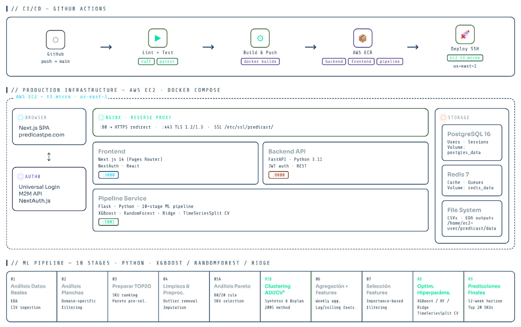
Figure 2.
(a) Average MAPE by company and dominant algorithm; (b) relationship between MAPE and R² for the 18 SKUs according to the selected algorithm.
Figure 2.
(a) Average MAPE by company and dominant algorithm; (b) relationship between MAPE and R² for the 18 SKUs according to the selected algorithm.
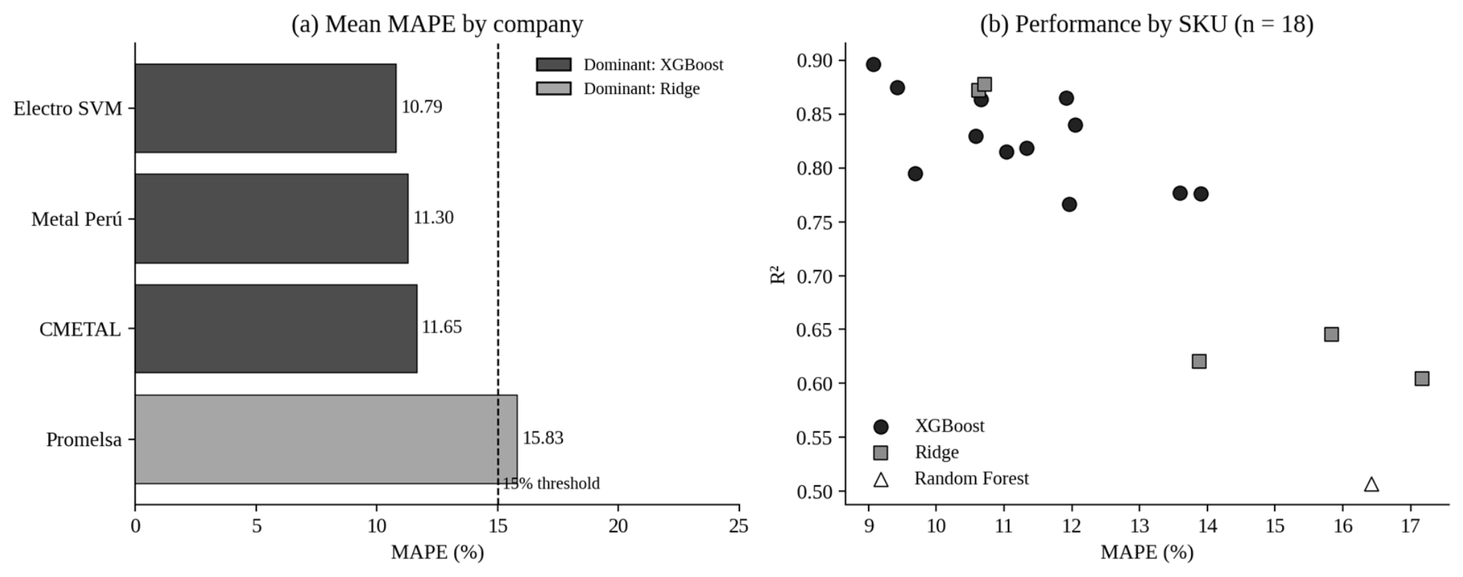
Figure 3.
Cross-validation R² of XGBoost, Random Forest, and Ridge by SKU and company.
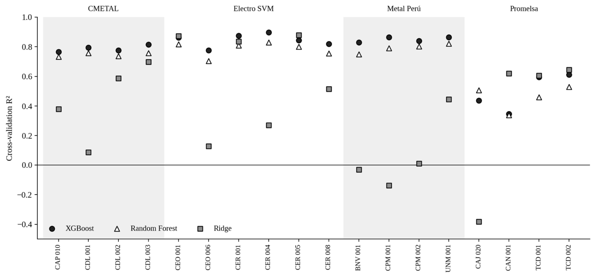
Figure 4.
MAPE per SKU of the winning model (pipeline configuration) and of three naïve baseline methods.
Figure 4.
MAPE per SKU of the winning model (pipeline configuration) and of three naïve baseline methods.
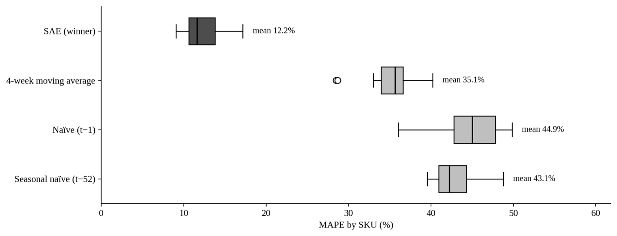
Figure 5.
Weekly demand over the last two years and 52-week recursive forecasting with a 95% confidence band: (top) CER 004 from Electro SVM; (bottom) TCD 001 from Promelsa.
Figure 5.
Weekly demand over the last two years and 52-week recursive forecasting with a 95% confidence band: (top) CER 004 from Electro SVM; (bottom) TCD 001 from Promelsa.
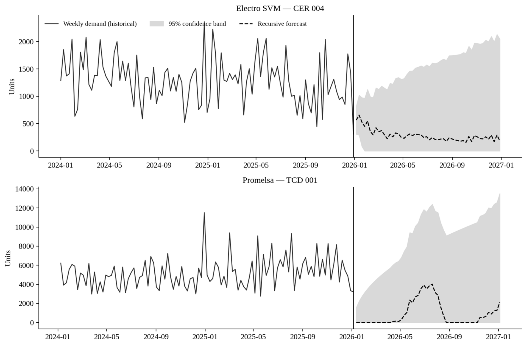
Table 1.
Comparison of the closest works.
| Work | Sector | Methods | ADI/CV² | Deployed System | Companies |
|---|---|---|---|---|---|
| Sukolkit et al. [10] | Steel | Prophet, SVR, CNN, RNN, GRU, LSTM | N/R | N/R | 1 |
| Obaidat et al. [33] | Dairy | XGBoost, SARIMAX | N/R | N/R | 1 |
| Ma et al. [14] | Beverages | Selection by SKU group | Other | N/R | 1 |
| da Silva et al. [25] | Energy (spare parts) | RF, XGBoost, Holt-Winters, SARIMA | Yes | N/R | 1 |
| Dodin et al. [34] | Aeronautics | ML and time series | N/R | Yes (in the company) | 1 |
| Kang et al. [27] | Manufacturing SME | Statistical, ML, and hybrid | N/R | No | 1 |
| Cruz Martins et al. [26] | Brewing SMEs | ML and operations research | N/R | N/R | Synthetic data |
| Fries et al. [28] | Metalworking | Qualitative study | No | Conceptual | 3 |
| This work | Metalworking (Peru) | XGBoost, RF, Ridge (SAE) | Yes | Yes (web, AWS) | 4 |
Note. N/R: not reported in the article; “Other”: classification by volume and volatility.
Table 2.
Source variables of the transactional dataset.
| Variable | Description |
|---|---|
| Código | SKU identifier |
| Fecha | Transaction date |
| Salida | Units sold (actual demand) |
| Saldo | Stock available at the time |
| Empresa_Cliente | Customer who made the purchase |
| Canal_Venta | Distribution channel (online / in-store) |
| Punto_Venta | Dispatch warehouse (Sector A / Sector B) |
Table 3.
Calendar and seasonal features.
| Feature | Description |
|---|---|
| Mes, Trimestre | Calendar variables |
| Semana_Sin, Semana_Cos | Fourier encoding of the ISO week |
| Mes_Sin, Mes_Cos | Fourier encoding of the month |
| Trim_1—Trim_4 | Quarter indicator variables |
| Día_Año, Num_Semana_Año | Position in the year |
Table 4.
Evaluated feature sets.
| Set | No. of features | Inclusion criterion |
|---|---|---|
| Conservative | 15 | Only lags, moving averages, volatilities, and ratios |
| Intermediate | 36 | The above plus customer, channel, and quarterly features |
| Aggressive | 48 | All available features |
Table 5.
Profile of the participating companies according to their public information.
| Company | Activity | Main product lines | Location |
|---|---|---|---|
| CMETAL Condulet Perú | Manufactures and distributes | Condulet boxes and covers, neoprene gaskets | San Isidro |
| Electro SVM | Manufactures and distributes | Flush-mount boxes (rectangular, octagonal, pull), raceways, DIN and Unistrut rails, panelboards | Cercado de Lima |
| Metal Perú S.A.C. | Manufactures and distributes | Cable trays and ladder trays, pull boxes, strut channels, supports | Lurín |
| Promelsa | Distributes | Cables, panelboards, conduit, trays, strut channels, junction and condulet boxes | La Victoria |
Source: corporate websites of the companies, synthesized with NotebookLM (September 2026). Locations in Metropolitan Lima and Callao.
Table 8.
ADI/CV² classification of the weekly series of the evaluated SKUs.
| Company | SKU | CV² | Company | SKU | CV² |
|---|---|---|---|---|---|
| CMETAL | CAP 010 | 0.164 | Electro SVM | CER 008 | 0.166 |
| CMETAL | CDL 001 | 0.143 | Metal Perú | BNV 001 | 0.152 |
| CMETAL | CDL 002 | 0.154 | Metal Perú | CPM 001 | 0.157 |
| CMETAL | CDL 003 | 0.164 | Metal Perú | CPM 002 | 0.171 |
| Electro SVM | CEO 001 | 0.138 | Metal Perú | UNM 001 | 0.149 |
| Electro SVM | CEO 006 | 0.171 | Promelsa | CAJ 020 | 0.222 |
| Electro SVM | CER 001 | 0.152 | Promelsa | CAN 001 | 0.187 |
| Electro SVM | CER 004 | 0.158 | Promelsa | TCD 001 | 0.195 |
| Electro SVM | CER 005 | 0.140 | Promelsa | TCD 002 | 0.195 |
Note. ADI = 1.00 for all SKUs. Syntetos and Boylan thresholds: ADI = 1.32, CV² = 0.49.
Table 9.
Cross-validation metrics by company (average over its SKUs).
| Company | MAPE (%) | RMSE | MAE | R² | Dominant algorithm | SKUs |
|---|---|---|---|---|---|---|
| Electro SVM | 10.79 | 236.97 | 179.19 | 0.8528 | XGBoost | 6 |
| Metal Perú S.A.C. | 11.30 | 236.39 | 173.93 | 0.8499 | XGBoost | 4 |
| CMETAL Condulet Perú | 11.65 | 462.06 | 336.98 | 0.7883 | XGBoost | 4 |
| Promelsa S.R.L. | 15.83 | 923.58 | 689.06 | 0.5943 | Ridge | 4 |
| Average | 12.39 | 464.75 | 344.79 | 0.7713 | — | 18 |
Source: authors’ own elaboration based on running the pipeline on the companies’ data (2021–2025).
Table 10.
Selection frequency and mean performance of the winning algorithm.
| Algorithm | SKUs won | % | Mean MAPE (%) | Mean R² |
|---|---|---|---|---|
| XGBoost | 12 | 66.7 | 11.27 | 0.827 |
| Ridge | 5 | 27.8 | 13.64 | 0.724 |
| Random Forest | 1 | 5.6 | 16.42 | 0.507 |
Table 11.
Results by SKU: cross-validation R² of the three algorithms and metrics of the winner.
| Company | SKU | R² XGB | R² RF | R² Ridge | Winner | MAPE (%) | RMSE | MAE |
|---|---|---|---|---|---|---|---|---|
| CMETAL | CAP 010 | 0.767 | 0.734 | 0.380 | XGB | 11.96 | 464.4 | 336.3 |
| CMETAL | CDL 001 | 0.795 | 0.757 | 0.086 | XGB | 9.68 | 540.6 | 388.4 |
| CMETAL | CDL 002 | 0.776 | 0.738 | 0.587 | XGB | 13.90 | 456.1 | 350.6 |
| CMETAL | CDL 003 | 0.815 | 0.757 | 0.698 | XGB | 11.03 | 387.1 | 272.6 |
| Electro SVM | CEO 001 | 0.862 | 0.818 | 0.872 | Ridge | 10.63 | 273.9 | 199.2 |
| Electro SVM | CEO 006 | 0.777 | 0.704 | 0.127 | XGB | 13.60 | 350.7 | 271.9 |
| Electro SVM | CER 001 | 0.875 | 0.808 | 0.836 | XGB | 9.42 | 237.0 | 178.0 |
| Electro SVM | CER 004 | 0.897 | 0.830 | 0.271 | XGB | 9.06 | 131.6 | 95.6 |
| Electro SVM | CER 005 | 0.844 | 0.801 | 0.878 | Ridge | 10.71 | 208.5 | 166.9 |
| Electro SVM | CER 008 | 0.818 | 0.755 | 0.516 | XGB | 11.34 | 220.1 | 163.4 |
| Metal Perú | BNV 001 | 0.830 | 0.750 | -0.032 | XGB | 10.58 | 203.8 | 150.9 |
| Metal Perú | CPM 001 | 0.865 | 0.791 | -0.138 | XGB | 11.92 | 311.8 | 223.1 |
| Metal Perú | CPM 002 | 0.840 | 0.803 | 0.009 | XGB | 12.05 | 209.7 | 153.9 |
| Metal Perú | UNM 001 | 0.864 | 0.820 | 0.446 | XGB | 10.66 | 220.2 | 167.8 |
| Promelsa | CAJ 020 | 0.437 | 0.507 | -0.382 | RF | 16.42 | 1390.1 | 1034.9 |
| Promelsa | CAN 001 | 0.347 | 0.339 | 0.620 | Ridge | 13.88 | 631.6 | 455.8 |
| Promelsa | TCD 001 | 0.596 | 0.459 | 0.605 | Ridge | 17.17 | 806.7 | 597.2 |
| Promelsa | TCD 002 | 0.611 | 0.529 | 0.645 | Ridge | 15.84 | 865.9 | 668.4 |
Source: authors’ own elaboration (TimeSeriesSplit, k = 5).
Table 12.
Sensitivity analysis: mean performance over the 18 SKUs according to the treatment of the forecast-week features.
Table 12.
Sensitivity analysis: mean performance over the 18 SKUs according to the treatment of the forecast-week features.
| Configuration | Mean MAPE | Median MAPE | Mean R² | Better than MA(4) | Winners |
|---|---|---|---|---|---|
| Repository pipeline | 12.21 | 11.63 | 0.780 | 18/18 | XGB 12, Ridge 5, RF 1 |
| Features lagged by one week (t − 1) | 34.59 | 34.19 | -0.258 | 10/18 | RF 18 |
| 4-week moving average | 35.13 | 35.68 | -0.164 | — | — |
Source: authors’ own elaboration. Same data, temporal folds, and hyperparameter grids in all three configurations.
Table 13.
Production efficiency indicators by SKU at the pilot company.
| SKU | Sheet | Produced | Sold | Over-prod. | Eff. | Excess RM cost (PEN) | Total impact (PEN) |
|---|---|---|---|---|---|---|---|
| CER 001 | F.G. 0.75 | 656,212 | 616,974 | 39,238 | 94.0% | 36,163 | 54,968 |
| CER 005 | F.G. 0.75 | 612,744 | 571,597 | 41,147 | 93.3% | 37,922 | 57,642 |
| CER 004 | F.G. 1.20 | 399,882 | 370,970 | 28,912 | 92.8% | 41,344 | 62,843 |
| CERE 002 | F.G. 1.20 | 264,085 | 247,482 | 16,603 | 93.7% | 23,742 | 36,088 |
| CEO 001 | F.G. 0.75 | 776,415 | 722,970 | 53,445 | 93.1% | 61,462 | 93,422 |
| CEO 006 | F.G. 0.75 | 698,074 | 652,698 | 45,376 | 93.5% | 52,182 | 79,317 |
| CER 008 | F.G. 1.20 | 484,674 | 447,689 | 36,985 | 92.4% | 64,846 | 98,566 |
| Total | — | — | — | 261,706 | 93.3% | 317,662 | 482,846 |
Source: authors’ own elaboration with transactional data from Corporación Electro SVM.
Table 15.
Results of user acceptance testing by company.
| Company | Participants | Tasks Completed without Assistance | Mean Time per Task (min) | Mean SUS | Mean Usefulness |
|---|---|---|---|---|---|
| Electro SVM (pilot) | 5 | 72.7% (8/11) | 4.2 | 69.5 | 4.10 |
| Metal Perú | 5 | 90.9% (10/11) | 3.5 | 81.5 | 4.17 |
| CMETAL | 5 | 72.7% (8/11) | 4.6 | 68.0 | 3.83 |
| Promelsa | 5 | 100% (11/11) | 3.0 | 84.0 | 4.43 |
| Total | 20 | 84.1% (37/44) | 3.8 | 75.8 | 4.13 |
| Criterion | — | ≥ 80% | Baseline | ≥ 68 | ≥ 4.0 |
Source: authors’ own elaboration from the questionnaires and task-recording sheets (19–22 October 2026).
Disclaimer/Publisher’s Note: The statements, opinions and data contained in all publications are solely those of the individual author(s) and contributor(s) and not of MDPI and/or the editor(s). MDPI and/or the editor(s) disclaim responsibility for any injury to people or property resulting from any ideas, methods, instructions or products referred to in the content. |
© 2026 by the authors. Licensee MDPI, Basel, Switzerland. This article is an open access article distributed under the terms and conditions of the Creative Commons Attribution (CC BY) license.
Copyright: This open access article is published under a Creative Commons CC BY 4.0 license, which permit the free download, distribution, and reuse, provided that the author and preprint are cited in any reuse.