
Submitted:
17 November 2026
Posted:
18 November 2026
You are already at the latest version
Abstract
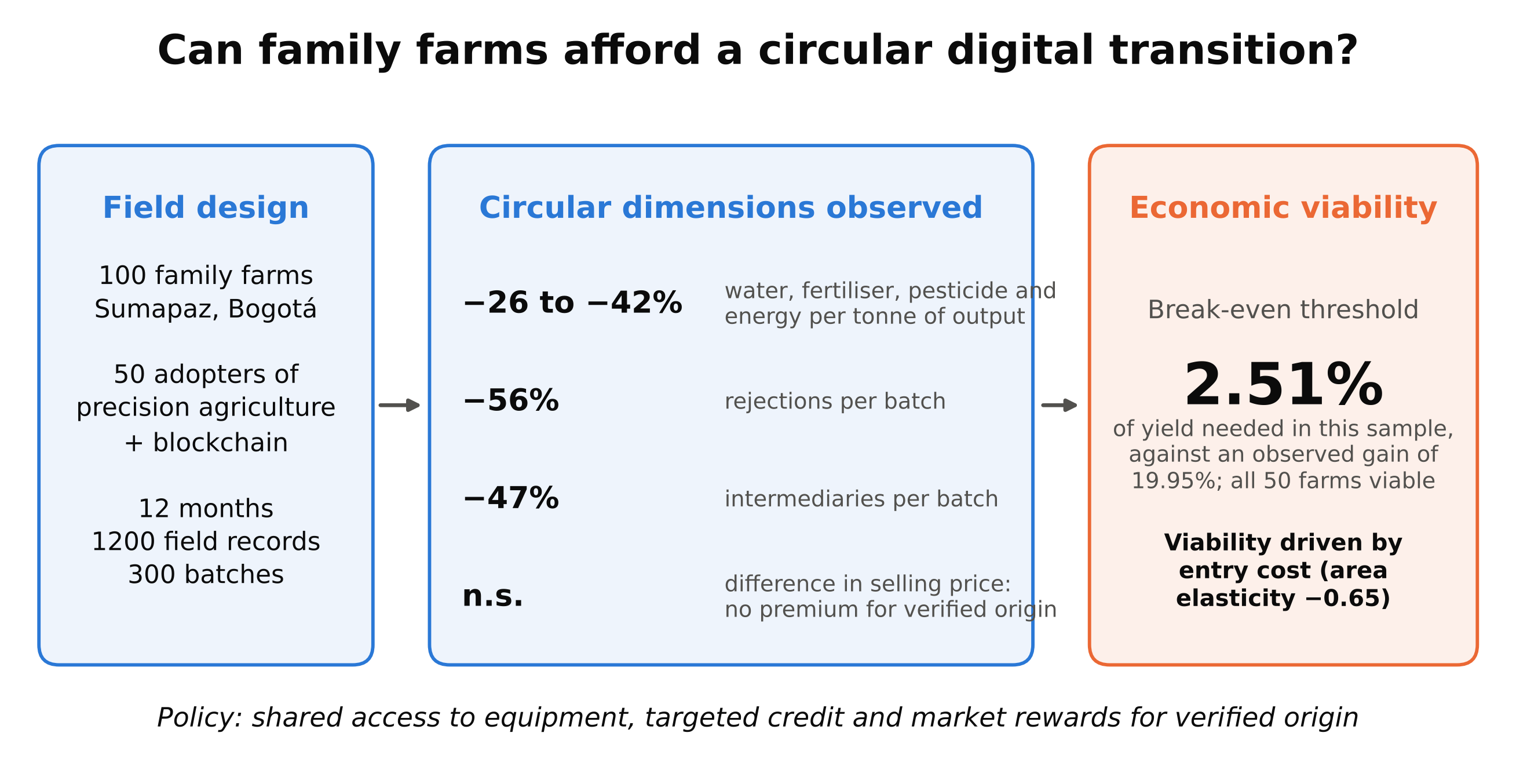
Digital technologies are promoted as enablers of circular agri-food systems, yet family farms lack tools to judge whether such investments pay off, and economic data at this scale are often unreliable. This study develops a break-even threshold framework that evaluates digital investments using only physical and price variables, derives three propositions on entry costs, decision robustness and unreliable data, and applies it to precision agriculture with blockchain traceability on 100 family farms in Sumapaz, Bogotá, Colombia, 50 of them adopters. Three circular dimensions were assessed: the narrowing of resource flows, value retention and chain governance. Adopting farms used 26 to 42% fewer inputs per tonne of output and recorded fewer batch rejections and intermediaries. The investment broke even with a yield gain of 2.51% against an observed differential of 19.95%, and all farms remained viable if only half of that differential were retained, if half of the additional output went unsold or if technology costs doubled. Viability depended on the ratio of investment to farm area, with an elasticity of −0.65, and no price premium for verified origin was found. The framework turns transition narratives into a computable decision rule and identifies entry cost as the main barrier for smallholders.
Keywords:
circular economy
; decision support
; resource efficiency
; precision agriculture
; blockchain traceability
; break-even analysis
; family farming
; value retention
; sustainability assessment
; Colombia
1. Introduction
Agri-food systems sit at the centre of current debates on circular economy and bioeconomy transitions. The circular economy concept has consolidated around the idea that resource value should be retained within production and consumption systems, while questions remain about how environmental and economic goals can be pursued together [1]. In agriculture, this idea has been translated into strategies that narrow, slow and close resource loops at farm level [2], and bioeconomy strategies increasingly frame biological production within a circular logic that values resource efficiency, residues and cascading uses [3,4]. Recent work has also framed the bioeconomy through the environmental, economic, social and governance pillars of sustainable development and as a matter of spatial planning [5]. Digital technologies appear in almost every version of these transition narratives as tools that could raise productivity, reduce input use and make agri-food chains more transparent [6,7,8,9,10,11], and the links between digitalisation and circular strategies have been mapped in industrial settings [12].
Two digital technologies carry most of these expectations in primary production. Precision agriculture combines sensors, positioning systems and decision platforms to match inputs and operations to the variability of the production system [13,14], while blockchain has been proposed as infrastructure that strengthens the integrity and verifiability of the information accompanying a product along the chain [15,16,17]. Their integration forms a coupled architecture in which the first layer acts on resource allocation within the farm and the second on the flow of information that allows the farm to be coordinated with buyers and verified by them. From a circular economy perspective, the first layer is expected to reduce the material and energy inputs needed per unit of output, which corresponds to what the literature calls narrowing resource flows [18], and the second is expected to support value retention, accountability and new forms of chain coordination [19,20,21,22].
The evidence behind these expectations remains uneven, since conceptual proposals, architectures and prototypes are far more common than evaluations of real agricultural implementations [23,24,25], and the field studies that exist tend to be exploratory and focused on specific performance indicators [26,27]. Empirical work on blockchain for the circular economy suggests that practitioners see the technology as an infrastructural resource that moderates the transition rather than as a solution in itself [21]. For precision agriculture, a recent meta-analysis found that economic and environmental benefits at farm level are weaker and less stable on small farms and in developing countries [28], even though systematic reviews of fertiliser management report clear reductions in environmental footprints when the technology is applied [29]. Evidence on technology bundles adds a further complication, because gains often depend on how tools are combined. In the United States, farms using advanced bundles of precision agriculture were more technically efficient than non-adopters [30], whereas within-farm panel data from Kansas showed gains for only a few bundles, concentrated on less efficient farms [31]. In Bolivia, neither improved rice varieties nor fertiliser raised yields when adopted alone, while their joint adoption almost doubled productivity [32]. For blockchain, ex-ante work with smallholder cocoa producers in Peru found that some sustainability attributes cannot be verified through digital tracing alone and that implementation challenges are highly context-specific [33].
Who can take part in a digital and circular transition is therefore as important as what the technology delivers. Access to digital infrastructure is strongly skewed by farm size, with only 24 to 37% of farms under 1 ha served by 3G or 4G networks against 74 to 80% of farms above 200 ha [34], and reviews of smallholder digital agriculture identify affordability, digital skills and underdeveloped digital ecosystems as persistent barriers [35]. Adoption cost, scalability and firm size appear among the critical determinants of blockchain implementation in food chains [36,37]. Precision agriculture remains limited in small-scale farming regions [38]. In Latin America, economic, financial and infrastructure constraints recur among the barriers to digital agriculture [39], and in Colombia a review of adoption studies found that producer and farm characteristics, together with perceived usefulness and ease of use, are the main determinants [40]. Adoption also responds to a broad set of farm-level and system-level determinants [41], and cost, together with farmers’ perceptions of what the technology delivers, shapes adoption decisions [42,43]. Profitability depends on scale, since net present value turns positive only above a certain economic farm size [44]. Critical reviews have examined the circular economy through the lens of inclusion and argued that a more inclusive society strengthens the transition [45]. The same concern appears in work on farmer inclusion in bioeconomy policy [46], on the inclusion and exclusion effects of Agriculture 4.0 technologies [10] and on policy visions of digital agriculture that prioritise maximising output [47]. These determinants, however, are rarely quantified against outcomes measured in the field.
Measuring the economics of such transitions at small scale raises a further difficulty. The magnitudes that bear on an adoption decision, such as income, consolidated costs and margins, are usually collected through recall-based interviews without documentary support. Recall-based agricultural data carry nonrandom measurement error that grows with the length of the recall period [48], farmer-reported production can differ substantially from objective measurements [49], and the methodological literature recommends collecting self-reported and objectively measured data for the same variable whenever feasible [50]. When return on investment is estimated from such declarations, the result displays a precision that the sources do not support, in a domain where the decision to invest falls on producers with constrained capital.
This study addresses both gaps by developing an assessment framework and applying it to records from Sumapaz, the rural locality of Bogotá, Colombia. Instead of estimating the return actually obtained, which requires income data whose validity is often doubtful at this scale, the framework determines the performance threshold, that is, the productivity gain needed for an investment in digital technology to break even, and reads it alongside indicators of resource efficiency, value retention and chain governance. The study pursues three objectives: to formalise the threshold framework and the propositions that follow from it; to apply it to a twelve-month quasi-experimental follow-up of 100 family farmers who did or did not adopt precision agriculture with blockchain traceability; and to test how far the resulting adoption decision withstands changes in discount rate, horizon, price and the size of the observed effect.
The study does not measure circularity as a whole. It evaluates three dimensions of a circular digital transition that can be observed with farm and batch records, namely the narrowing of resource flows, value retention and chain governance, and treats closing and slowing loops as a research agenda. Within that scope, it makes three contributions. First, it extends the argument on fixed costs and indivisible technologies to digital packages and shows, farm by farm, how entry cost filters participation. Second, it states an adoption decision rule that remains valid without full identification of the effect, together with a stress test of how much error the decision can absorb. Third, it proposes an evaluation procedure that relies only on verifiable physical and price variables, which suits family-farming programmes whose economic survey data are unreliable. The result is a replicable decision-support tool, in the sense discussed for Agriculture 4.0 [51], for a country that has adopted bioeconomy policies and regional bioeconomy ambitions [52,53,54]. Section 2 describes the design, the data, the conceptual framework and the model. Section 3 reports the resource, chain and threshold results. Section 4 discusses them in relation to circular economy and bioeconomy transitions, and Section 5 concludes.
2. Materials and Methods
2.1. Study Design and Setting
The study used data from an applied quasi-experimental design with two parallel groups and twelve months of longitudinal follow-up, conducted with 100 adult family farmers in five rural settlements (veredas) of Sumapaz: Betania, La Unión, Las Ánimas, Nazareth and San Juan. Fifty farmers formed the adopting group, which operated precision agriculture systems integrated with blockchain traceability, and fifty continued with their usual practices. The crops represented were pea, onion, potato and leafy vegetables, and allocation to groups was not random. All participants completed the follow-up, which yielded 1200 monthly field records and 300 batch records.
The groups were comparable at baseline in age (47.70 ± 13.12 and 49.26 ± 12.56 years in the adopting and comparison groups; p = 0.545), total farm area (6.46 ± 3.27 and 7.27 ± 3.05 ha; p = 0.205), study plot area (3.67 ± 1.57 and 3.43 ± 1.55 ha; p = 0.448), sex (p = 0.839), education level (p = 0.673) and main crop (p = 0.298). Farming experience was lower in the adopting group (16.94 ± 9.78 years) than in the comparison group (21.48 ± 8.77 years; p = 0.016) and was therefore included as a covariate in the robustness analysis. The comparison group was not entirely free of digital tools, since 16 of its 50 farmers reported prior use of some precision agriculture component and 52 of its 150 batches carried an origin that consumers could verify. This partial exposure works against finding differences between groups, and Section 3.9 reports the main contrasts with these 16 farmers excluded.
The technology package combined field sensing, positioning and data platforms with blockchain registration of each commercial batch. According to the participant records, all 50 adopting farms used sensors, GPS or GIS tools and internet-of-things devices, 39 used smart irrigation and 26 used drones. In the comparison group, 17 farms used some sensors and 27 used GPS or GIS tools, while none used internet-of-things devices, smart irrigation or drones. Every batch of the adopting group was registered on the blockchain platform and carried a QR code with which consumers could verify its origin.
2.2. Conceptual Framework
The analysis follows the distinction between narrowing, slowing and closing resource loops proposed for circular business models [18] and adapted to agricultural production systems [2]. Figure 1 summarises how the study connects these strategies with economic viability. Three channels can be observed with the available records: the narrowing of resource flows, measured as inputs per tonne of output; value retention along the chain, measured through batch rejections, product recall time and record errors; and chain governance, measured through the number of intermediaries, buyer type and the presence of a price premium. These channels feed into the break-even threshold, whose distribution across farms reveals the distributional filter created by entry costs and points to the policy mixes that could widen participation. Closing loops through residue and nutrient recovery, slowing loops, cascading uses and bio-based value chains were not measured and are treated as a research agenda rather than as findings.
2.3. Information Sources and Prior Verification
The data come from three instruments of differing nature and reliability, and that distinction shapes the analysis. The monthly field record produced 1200 observations, twelve per participant, covering yield, cultivated area, total output and the use of water, fertiliser, pesticide, energy and labour. Its internal identities were verified, since total output reproduces the product of yield and area with a maximum relative error of 0.00001 and total water use reproduces per-hectare use multiplied by area with a maximum error of 0.00022. The batch record covered 300 batches, three per participant, with harvest date, traceability indicators, product recall time, record errors, data discrepancies, rejections, number of intermediaries, buyer type and selling price per kilogram.
The direct economic survey collected, through recall-based interviews without documentary support, the annual cost structure by item, annual income, gross margin and initial technology investment. This instrument is internally coherent, because its cost components sum exactly to total cost and the difference between income and cost reproduces the margin, but it cannot be reconciled with the field record. At participant level, reported income is not associated with measured output (r = 0.08 in the adopting group and 0.03 in the comparison group) or with the price recorded at batch level (r = −0.08 and −0.03), and consolidated cost is not associated with the operating cost derived from the monthly record (r = −0.25 and −0.02). The ratio between measured output and the output implied by reported income varies by a factor of about three across participants (from 5.4 to 16.7 when measured output is taken per monthly record), which rules out a simple problem of scale or time unit.
The analysis used the original database of the project, compiled by the principal investigator during the fieldwork, which contains the participant, monthly field, batch and economic survey records. The records do not specify whether each monthly yield value corresponds to a single harvest or to accumulated output, so the model adopts the conservative interpretation described in Section 2.6. The internal consistency checks reported above were carried out before any analysis, and the anonymised database is provided as Supplementary File S2.
This pattern agrees with the literature on recall error in agricultural surveys [48,49], and the design allows the comparison between self-reported and measured data that has been recommended for this kind of evaluation [50]. Income, consolidated total cost and gross margin were therefore excluded from the analysis. From the survey, only the initial technology investment and the recurring technology costs were retained, because they correspond to discrete and recent outlays and no alternative source exists for them. The sensitivity of the conclusions to errors in these costs is assessed through the maximum justifiable initial investment.
2.4. Resource Efficiency and Chain Indicators
Resource efficiency was expressed as input intensity per tonne of output, a measure that captures the narrowing of resource flows more directly than input use per hectare because it accounts for the yield response at the same time. For each participant, the twelve monthly values of water, fertiliser, pesticide, energy and labour use per hectare were summed and divided by the sum of the twelve monthly yields per hectare, giving cubic metres, kilograms, litres, kilowatt-hours and hours per tonne. Chain indicators were averaged over the three batches of each participant. They include the share of the product traceable from farm to buyer, the time needed to trace a batch, the time needed to recall a product, the number of record errors and data discrepancies, the number of rejections per batch, the number of intermediaries and the delivery time.
2.5. Model Parameters
The threshold model uses four observed parameters and two set by the authors (Table 1). The recurring technology cost combines the operating cost of the blockchain platform and equipment maintenance. Technology subscription was excluded from the incremental cost because the comparison group also reports it, at a slightly higher mean value (69,619 against 65,783 COP/ha per year).
2.6. Threshold Specification
For each farm i, the investment was annualised with the capital recovery factor
and the annual technology cost per hectare was obtained as
where Ri is the recurring cost per hectare, Ii the initial investment and Ai the study plot area. The additional output required to break even is
with Pi the mean selling price of the farm. The relative threshold was expressed with respect to the mean yield of the comparison group,
and the coverage ratio as the quotient of the observed advantage and the threshold,
CRF(r, N) = r(1 + r)N / [(1 + r)N − 1],
Ci = Ri + Ii · CRF(r, N) / Ai,
Δq*i = Ci / Pi,
δ*i = Δq*i / ȳc,
Ki = (ȳi − ȳc) / Δq*i.
The ratio of the relative threshold to the observed relative differential gives the minimum fraction of the yield advantage that would have to be attributable to the intervention for the investment to break even. At farm level, this fraction equals 1/Ki. Yield enters the model as the participant mean of the twelve monthly records and is treated as the yield of one annual production cycle, while technology costs are annual. This choice is conservative, because if each record corresponded to a separate harvest, annual output would be larger, the relative threshold smaller and the coverage ratio higher. Appendix A (Table A2) reports the model under two, three and twelve cycles per year to show the size of this margin.
2.7. Analytical Propositions
The specification yields three propositions. Their mathematical content is elementary, and their contribution lies in what they imply for evaluating digital investments on small farms, which is discussed after they are stated. Combining Equations (2) to (4), the relative threshold can be written as
δ*i = [Ri + Ii · CRF(r, N) / Ai] / (Pi · ȳc).
Proposition 1 (structural viability).The threshold rises with the initial investment and the recurring cost and falls with the selling price and with the plot area. In particular,
and the elasticity of the threshold with respect to area equals minus the share of the annualised investment in the annual technology cost,
∂δ*i / ∂Ai = −Ii · CRF(r, N) / (Ai2 · Pi · ȳc) < 0,
εi = −[Ii · CRF(r, N) / Ai] / Ci.
When technology costs are dominated by a fixed investment, viability therefore depends on the ratio of investment to area rather than on the agronomic response, and differences in viability across farms are expected to reflect differences in entry cost.
Proposition 2 (decision robustness under non-random assignment).For an adoption decision, the relevant quantity is not the causal effect itself but whether it exceeds the threshold. The ratio δ*i/δi, equal to 1/Ki, is the minimum share of the observed differential that must be causal for the decision to hold, so a conclusion about viability can be robust even when the effect is not fully identified.
Proposition 3 (evaluation under unreliable economic data).Equation (6) involves only investment, recurring cost, price, area and yield. Where survey-based economic data cannot be reconciled with physical measurements, reformulating the evaluation as a threshold problem preserves the economic question while relying only on verifiable variables.
These properties follow directly from Equation (6), so their value does not lie in the derivation. Proposition 1 extends to digital technologies the long-standing argument that fixed costs make the adoption of indivisible technologies sensitive to farm size [55], and adds that, because digital packages combine an indivisible equipment layer with recurring per-hectare costs, the sensitivity to area is bounded by the share of the investment in the annual cost and can be computed for each farm. Proposition 2 changes the object of evaluation from the size of an effect to whether the effect clears a threshold. In observational designs, where every adjustment rests on assumptions that cannot be fully tested [56], this allows a decision to be stated together with the share of the effect that would have to be spurious to overturn it. Proposition 3 makes the choice of variables part of the design, so that the economic question is answered with the information whose validity can be checked rather than with the information that happens to be available.
2.8. Sources of Heterogeneity
To identify the sources of heterogeneity in coverage, the variance of log Ki was decomposed into the covariance contributions of its three additive components, the log yield advantage, the negative log annualised cost and the log selling price. Since log Ki = log(ȳi − ȳc) − log Ci + log Pi, the variance decomposes exactly as
and each term divided by Var(log Ki) gives the share of the variance attributable to that component. Spearman rank correlations were also computed between the coverage ratio and each model input.
Var(log Ki) = Cov[log(ȳi − ȳc), log Ki] + Cov(−log Ci, log Ki) + Cov(log Pi, log Ki),
2.9. Scenarios and Sensitivity Analysis
The reference scenario uses a discount rate of 12% and a five-year horizon. Rates of up to 18% represent the higher discount rates that private producers may face, and lower rates represent the opportunity cost of public funds. Rates of 0, 8, 12, 15 and 18% and horizons of 3, 5, 7 and 10 years were evaluated, together with variations in the selling price between 50 and 150% of the observed value. A stress test then recomputed the share of farms that break even when only a fraction of the observed yield differential is retained, from 0 to 100%, which shows how much measurement error or confounding the adoption decision can absorb. The minimum price that sustains the investment and the maximum justifiable initial investment given the observed yield differential were also estimated. Further scenarios relaxed the assumptions on which the model is most optimistic: the share of the additional output that is actually sold (100, 75, 50 and 40%), joint increases of 25, 50 and 100% in initial investment and recurring cost, the replacement of 50 or 100% of the equipment in the third year, and combinations of these changes (Appendix A, Table A2).
2.10. Statistical Treatment
All group comparisons were made at participant level, aggregating each farmer’s monthly or batch records to avoid treating repeated observations as independent, and were tested with Welch’s t-test, 95% confidence intervals and Hedges’ g. The yield differential was re-estimated by ordinary least squares with heteroskedasticity-robust HC3 standard errors [57], adjusting for farming experience, study plot area and main crop. The threshold was computed farm by farm and is reported as a distribution, and both aggregation procedures, the mean of individual ratios and the ratio of group means, are reported because they differ. No inference was performed on variables from the economic survey. Three robustness checks were applied to all outcomes. First, a propensity score was estimated by logistic regression of adoption on age, total farm area, plot area, farming experience, education level, main crop and sex, and differences were re-estimated with inverse probability weights for the effect on adopters and HC3 standard errors. Overlap was assessed through the distribution of the propensity score in each group, the common support, the largest weight and the effective sample size of the weighted comparison group, following current guidance on weighting diagnostics [56,58], and the weighted estimate was repeated within the common support. Second, each adopting farm was matched with replacement to the comparison farm with the closest propensity score. Third, the comparisons were repeated after excluding the 16 comparison farmers who reported prior use of precision agriculture. Because fourteen outcomes were tested, p-values were also adjusted with the Holm procedure. Analyses were carried out in IBM SPSS Statistics 27 and Python 3.11. The threshold model, with editable parameters and the farm-level data required to reproduce the results, is provided as Supplementary File S1.
Generative artificial intelligence (Claude, Anthropic; Claude Opus 5.5) was used as an assistant under the direction of the authors to write the Python code for the analyses and figures, and to support the writing and English translation of the manuscript. The authors designed the study, collected the data and reviewed all outputs against the original database and Supplementary Files S1 and S2.
3. Results
3.1. Productivity Differential
Mean yield per record was 8468.83 ± 187.27 kg/ha in the adopting group and 7060.11 ± 197.45 kg/ha in the comparison group. The difference of 1408.71 kg/ha (95% CI 1332.34 to 1485.09) was statistically significant (t = 36.60; df = 97.7; p < 0.001), with a Hedges’ g of 7.26 that reflects the low dispersion of participant-level means within each group (coefficients of variation of 2.2 and 2.8%), since each value averages twelve monthly records. This corresponds to a relative differential of 19.95%. Adjusting for farming experience, study plot area and main crop left the estimate almost unchanged (1404.27 kg/ha; 95% CI 1321.85 to 1486.68; p < 0.001), and farming experience itself was not associated with yield (p = 0.380). This differential is the gross benefit against which the threshold is assessed.
3.2. Narrowing of Resource Flows
Higher yields came with lower input use. Per hectare, the adopting group used 17.4% less water (430.75 against 521.25 m3/ha), 19.0% less fertiliser (178.95 against 220.91 kg/ha), 30.1% less pesticide (6.98 against 9.98 L/ha), 15.4% fewer labour hours (74.71 against 88.31 h/ha) and 11.8% less energy (84.42 against 95.71 kWh/ha), all with p < 0.001. Because output rose at the same time, the reductions are larger when expressed per tonne of product (Figure 2 and Table 2). Water use fell by 31.1%, fertiliser by 32.5%, pesticide by 41.7%, energy by 26.5% and labour by 29.5% per tonne, and the two groups barely overlapped on any of the five indicators. These figures describe input use per unit of output. They are not estimates of environmental impact, which would also require emission factors, leaching and run-off measurements or a life-cycle inventory that the records do not contain.
3.3. Value Retention and Chain Governance
The batch record shows that adoption changed how product and information moved along the chain (Table 2). The share of product traceable from farm to buyer rose from 67.6 to 95.8%, the time needed to trace a batch fell from 11.5 to 1.2 h and the time needed to recall a product fell from 22.1 to 2.3 h. Record errors and data discrepancies were four to five times less frequent. Rejections per batch fell from 0.99 to 0.43, a reduction of 56.1% that points to less product leaving the commercial chain. Adopting farms sold through 1.9 intermediaries on average against 3.5 in the comparison group, while delivery time (p = 0.723) and the mix of buyer types (χ2 = 1.79; p = 0.408) did not differ. The mean selling price did not differ either (2870 against 2961 COP/kg; p = 0.218), so a shorter and better documented chain did not translate into a price premium in this sample.
3.4. Break-Even Threshold in the Reference Scenario
Initial investment varied widely, and the farm that invested most spent 3.7 times as much as the farm that invested least. At a discount rate of 12% and a five-year horizon, the annualised technology cost was 501,375 ± 266,614 COP/ha (range 201,067 to 1,577,535). The additional output required to break even was 177.6 ± 101.0 kg/ha per year, with a median of 146.4 and a range of 82.3 to 611.8. Expressed as a share of the comparison group’s yield, the threshold was 2.51 ± 1.43%, ranging from 1.17 to 8.67%. Against the observed differential of 19.95%, the mean coverage ratio was 9.70 ± 3.86, with a median of 9.82 and a minimum of 2.17.
All 50 adopting farms exceeded their own threshold (Figure 3). Even the least favoured farm, which combined the smallest plot in the sample (0.84 ha) with a high investment and a below-average price, obtained a yield advantage 2.17 times greater than required. The ratio of the relative threshold to the observed differential (2.51/19.95) indicates that, for the average farm, only 12.6% of the yield advantage would need to be attributable to the intervention for the investment to break even. Computed farm by farm as 1/Ki, this minimum attributable fraction had a mean of 12.9% and a median of 10.2% and reached 46.1% on the least favoured farm, so the conclusion holds for every farm as long as at least 46.1% of the observed differential is due to the intervention.
3.5. Sources of Heterogeneity and the Role of Farm Size
The decomposition of the variance of the log coverage ratio attributed 85.1% to the annualised technology cost, which combines initial investment, plot area and recurring cost, 10.0% to the yield advantage and 4.9% to the selling price. Investment per hectare was the input most strongly associated with coverage (Spearman ρ = −0.82; p < 0.001), followed by plot area (ρ = 0.59; p < 0.001) and total investment (ρ = −0.56; p < 0.001). The yield advantage showed a weaker association (ρ = 0.34; p = 0.015), and the selling price showed none (ρ = 0.16; p = 0.271).
Consistent with Proposition 1, the annualised investment accounted for 65.3% of the annual technology cost on average (median 66.0%; range 38.5 to 88.2%), so the elasticity of the threshold with respect to plot area averaged −0.65 and ranged from −0.38 to −0.88. On the average farm, a 10% larger area lowers the threshold by about 6.5%. Figure 4 shows this relationship as a viability frontier. For a farm with the median investment, recurring cost and price, the threshold rises from 1.9% of the comparison yield at 4 ha to 5.4% at 1 ha, and it would reach the observed mean differential only on plots of about a quarter of a hectare. The farms whose thresholds lie well above the median curve are those that combined small plots with investments above the median.
3.6. Sensitivity to Discount Rate and Horizon
The threshold remained between 1.38 and 3.68% across the twenty combinations evaluated (Table 3 and Figure 5a). In the most demanding scenario, a three-year horizon at 18%, the requirement of 3.68% is less than one fifth of the observed differential. The horizon proved more decisive than the discount rate. Moving from 0 to 18% raises the threshold by 0.81 percentage points at three years, whereas shortening the horizon from ten to three years at 18% raises it by 1.52 points.
3.7. Sensitivity to Selling Price and Derived Thresholds
Under the observed differential, the investment remained viable on all 50 farms even with the price halved (Table 4 and Figure 5b), although in that scenario the least favoured farm stood almost at break-even, with a coverage ratio of 1.09. Its own break-even price was 1188 COP/kg, which marks the lower limit of the result in this sample. Across farms, the minimum price that sustains the investment averaged 365 COP/kg (range 146 to 1188), equivalent to 12.7% of the mean observed price. The maximum justifiable initial investment, given the observed differential and prices, averaged about 51.0 million COP per farm, roughly 15.8 times the investment actually made, and the lowest ratio of justifiable to actual investment was 2.3.
3.8. Crops and Aggregation Procedures
The four crops showed thresholds within a narrow interval, between 2.09 and 2.82%, and coverage ratios between 8.78 and 11.75 (Table 5). Given the small number of farms per crop, these differences are descriptive rather than evidence of a differential effect. The results above average the ratios computed farm by farm. Deriving the threshold from group means instead gives 2.06% in the reference scenario, against 2.51%, a gap that reflects the skewed distribution of investment. The farm-level procedure was retained because it is more conservative and preserves the individual distribution that the distributional analysis requires.
3.9. Robustness Checks
The results did not depend on how the comparison was constructed (Appendix A, Table A1). The propensity score model balanced the observed characteristics, reducing the largest standardised mean difference, that of farming experience, from −0.49 to −0.02, and all standardised differences after weighting were below 0.08 in absolute value. Overlap was adequate (Appendix A, Table A3). Propensity scores ranged from 0.10 to 0.89 among adopters and from 0.09 to 0.82 among comparison farms, 49 farms of each group lay within the common support, the largest weight was 4.66, and the weighted comparison group had an effective size of 26.9 farms. With inverse probability weighting, the yield differential was 1427.86 kg/ha (95% CI 1341.34 to 1514.37), equivalent to 20.22%, restricting it to the common support gave 20.19%, and nearest-neighbour matching gave 20.83%. Excluding the 16 comparison farmers with prior precision agriculture gave 20.03%. Input intensities per tonne fell by 26 to 44% across the three checks, and the chain indicators kept their direction and size. The selling price remained without significant differences in every specification. All differences that were significant in the main analysis remained significant at p < 0.001 after Holm adjustment. Under the weighted and the restricted comparisons the mean threshold stayed at 2.52%, the minimum coverage ratio at 2.20 and 2.18, and all 50 farms remained viable.
3.10. Stress Test of the Adoption Decision
Figure 6 shows how many farms would still break even if only part of the observed yield differential were real. In the reference scenario, all 50 farms remain viable when half of the differential is retained, 45 farms (90%) remain viable with 22.7% of it, and half of the farms remain viable with about 10%. Under the most demanding combination of an 18% rate and a three-year horizon, 49 of 50 farms remain viable with half of the differential and all 50 with 72.7% of it. Combining that scenario with a selling price halved, and keeping the full differential, 49 farms still break even and only the least favoured farm falls below break-even, with a coverage ratio of 0.69. The adoption decision therefore tolerates large errors in the estimated effect, which is the property that makes the framework useful when field records are incomplete or the effect is not fully identified.
The decision also withstood changes in the assumptions that favour viability (Appendix A, Table A2). If only half of the additional output were sold, the required yield gain would rise to 5.02% and every farm would still break even, with a minimum coverage ratio of 1.09; with 40% sold, 49 farms would. Doubling both the initial investment and the recurring cost raised the threshold to 5.03% without making any farm unviable, and replacing all the equipment in the third year raised it to 3.78% with a minimum coverage of 1.34. The decision began to fail only when several adverse assumptions were combined. With half of the output sold and costs 50% higher, 49 farms remained viable, with costs doubled 46, and adding full equipment replacement to the first combination left 43. Conversely, if each monthly record corresponded to a separate harvest, the threshold would fall to 0.21% of annual output, so the one-cycle interpretation used throughout is the most demanding one.
4. Discussion
4.1. What a 2.5% Threshold Means for a Circular Digital Transition
The framework was designed to answer a practical question with the data that family-farming programmes actually hold, and its application shows that the answer can be robust even when the data are imperfect. The central economic result is that the technology package breaks even with a productivity gain of 2.51% in the reference scenario and that this requirement stays below 3.7% across all combinations of rate and horizon. The figure itself belongs to the costs, prices, plot sizes and yields of this sample and is not a general benchmark. What transfers is the procedure, because a producer or programme in another territory cannot assume the differential documented here but can compute its own threshold with Equation (6) and compare it with the gain it can reasonably expect. That comparison is the decision actually faced by anyone considering adoption, and it addresses the cost and scalability concerns that reviews of blockchain adoption in food chains leave unresolved [36,37]. Table 6 places the study within recent evidence. Most previous work on blockchain and the circular economy is conceptual, review-based or built on expert interviews, while field evaluations of precision agriculture rarely connect resource outcomes with a decision rule for small farms. International evidence on bundles also shows that gains vary widely, from higher technical efficiency among adopters of advanced bundles in the United States [30] to average gains for only a few bundles in Kansas, concentrated on less efficient farms [31]. The size of the differential in Sumapaz may reflect a starting point with more room for improvement, which is plausible in family farming with little prior technology but could not be tested here. Joint adoption effects of a similar order have been documented in Latin American smallholder systems [32], although for a different technology package.
4.2. Narrowing Resource Flows and Value Retention in a Smallholder Chain
The reductions of 26 to 42% in inputs per tonne correspond to the narrowing of resource flows, the circular strategy that seeks to use fewer resources per unit of product [2,18]. They are consistent with evidence that precision management lowers fertiliser use and environmental footprints [28,29] and with the expectation that digital agriculture can reconcile productivity with lower environmental pressure [8,9]. The finding matters for the circular agenda because it was obtained on family farms of a few hectares, a scale at which such benefits have been reported as weaker and less stable [28]. The input reductions should still be read as associations measured under the same design that produced the yield differential, not as separately identified causal effects, and as changes in input intensity rather than in environmental impact, which depends on how and where those inputs are lost to the environment.
The chain indicators add a second circular dimension. Fewer rejections, faster recall and fewer record errors mean that less product leaves the commercial chain and that problems can be located before they spread, which is the kind of value retention that digital monitoring is expected to deliver in food chains [59,60]. Some attributes of interest for sustainability, however, cannot be verified through digital records alone [33]. Blockchain did not act alone here, and the pattern agrees with the view that it works as infrastructure that supports circular practices rather than as a circular practice in itself [19,21]. Whether these gains translate into lower food losses in physical terms remains to be measured, because the batch record counts rejections but not the quantities rejected.
4.3. Attribution and the Magnitude of the Coverage Ratio
A coverage ratio close to ten calls for an explanation, since its size might be taken for a computational artefact. Its origin is a scale asymmetry, since the annualised technology cost is about half a million pesos per hectare per year, whereas the yield differential valued at the recorded price exceeds four million. Because the relative threshold equals 12.6% of the observed differential, the conclusion holds for the average farm even if only that fraction of the advantage were due to the intervention. This matters because the main objection to a quasi-experimental design is attribution, since technology adoption is subject to self-selection [61]. In the terms of Proposition 2, the adoption decision is robust to any degree of confounding that leaves at least 46.1% of the observed differential attributable to the intervention. Invalidating the conclusion for the average farm would require that more than 87% of the differential came from factors unrelated to the intervention, and 53.9% for the least favoured farm. The design cannot rule this out, but the differential was stable after regression adjustment, propensity score weighting, matching and the exclusion of exposed comparison farmers (Section 3.9), and it appeared together with lower input use and better chain performance on the same farms. These checks only address observed characteristics [56], so unobserved differences in management ability or motivation remain possible.
4.4. Entry Cost as a Distributional Filter
The farm-level distribution shows what group means conceal. Yield advantages were fairly homogeneous, between about 950 and 1820 kg/ha, while thresholds ranged from 82 to 612 kg/ha, a span of more than sevenfold. The annualised technology cost explained 85.1% of the variance in log coverage, and the least favoured farm was also the smallest. This is the empirical counterpart of Proposition 1 and of the classic argument on fixed costs and indivisible technologies [55]. In a circular transition, entry cost therefore acts as a distributional filter, since it decides who can capture the resource and chain benefits documented above. This connects the results with concerns about inclusion in circular economy and bioeconomy transitions [45,46] and with the digital divide that separates small from large farms [34,35].
If the critical variability lies in investment rather than in productive response, the most useful policy instruments are those that reduce or share the entry barrier, such as targeted credit, cooperative purchase of equipment, service-based rather than ownership-based access and shared infrastructure among neighbouring producers. Hire-service models allow smallholders to use equipment they could not afford to own, and digital platforms can lower the transaction costs of such services when connectivity and digital skills are in place [62]. Access-based models of this kind are also recognised as circular business models in their own right [18], and policy frameworks for the circular economy organise more than one hundred instruments that governments can combine for this purpose [63]. The interpretation agrees with evidence that net present value turns positive only above a certain farm size [44] and with arguments that public incentives for precision farming can be justified in small-scale farming systems of developing countries [13]. The viability frontier in Figure 4 offers a direct way to target such support, because it shows for any combination of investment and area how far a farm is from break-even.
4.5. Markets, Governance and Price Risk
Adoption shortened the chain without raising the price. This result is relevant for chain governance, because it shows that information quality and fewer intermediaries do not by themselves create a reward for verified origin. Premiums have been documented where traceability reaches export markets. In Ethiopia, the export price of traceable coffee rose by US$0.66 per kilogram more than that of non-traceable coffee [64], and in Colombia a segment of consumers was willing to pay on average 40.2% more for beef certified to environmental and animal welfare standards [65]. The local channels of Sumapaz appear to lack a comparable mechanism. Agricultural prices are volatile, with consequences for producers along the whole value chain [66], and the prices of micronutrient-dense foods such as vegetables have been found more volatile than those of starchy staples in developing countries [67]. The least favoured farm would cross break-even at about 1188 COP/kg, so the technology improves productivity and information but does not shield the producer from price variation. Economic evaluations of digital traceability should therefore include market risk explicitly, something the traceability literature tends to omit when it concentrates on the informational properties of the system [16,17].
4.6. Implications for Bioeconomy Governance in Colombia
Colombia has developed bioeconomy policies and indicators at national and regional levels [52], but regional expectations about bioeconomic potential are uneven and depend on how investment is channelled [53]. Decision support procedures have been proposed to prioritise bioeconomy investments by combining national indicators, regional features and stakeholder views [54]. The threshold and the viability frontier fit within that type of procedure at farm scale, since they turn a transition narrative into a criterion that can be computed with data a programme already collects. They also respond to calls for bioeconomy strategies supported by planning, clearer governance and engagement with local stakeholders [5,46]. In a territory of family farms such as Sumapaz, a programme that subsidised or shared the fixed investment would widen participation more than one focused on refining the technology package. Once access is secured, the next step towards a circular bioeconomy would be to connect these farms with residue valorisation and agro-waste business models [3,68], which this study did not observe.
4.7. Methodological Implication
Beyond the numerical result, the study illustrates a recurrent problem in the economic evaluation of agricultural technology at small scale. Income and consolidated cost data obtained by recall did not correspond to output measured in the field, and estimating return on investment from them would have produced figures that look precise but cannot be checked. The alternative adopted here establishes the threshold that physical evidence must exceed, using only the variables whose internal validity could be confirmed. As stated in Proposition 3, the procedure is not specific to precision agriculture or blockchain and applies to any technology whose costs are recorded more reliably than the income it generates. It also puts into practice the recommendation to collect self-reported and measured data for the same variable [50]. The stress test adds a further safeguard, since it tells the reader how much of an observed effect could be error before the decision changes, a property that matters most when records are incomplete, as they were here.
4.8. Limitations
The design did not include random assignment, so the yield differential, the input reductions and the chain improvements are associations rather than established causal effects, and the threshold analysis inherits that condition even though Section 4.3 limits its bearing on the conclusion. Part of the comparison group already used some digital tools, although excluding these farmers left the results practically unchanged. The model assumes that the additional output is sold in full at the observed price. The database does not record the volume marketed per batch, so the share actually sold, post-harvest losses and on-farm consumption could not be verified. This assumption operates in an optimistic direction, although all farms remained viable with half of the additional output sold (Table A2).
The intervention combined precision agriculture and blockchain traceability, so the design cannot separate their contributions. It is plausible that input reductions relate mainly to precision management and chain indicators mainly to traceability, but this is an interpretation, and the threshold refers to the package as a whole. Studies of technology bundles show that the effects of joint adoption can differ from those of each component [30,32], which makes factorial or staggered designs a priority for future evaluations.
Field procedures are reported at the level of detail contained in the project records. The differences between groups are also large and the dispersion within groups is small, which is unusual for smallholder data. The internal identities of the records hold, the comparison groups were balanced on observed characteristics and the results were stable across all robustness checks, but replication in other territories and with other technological configurations is needed before the magnitudes reported here are generalised.
Technology costs and initial investment come from the same survey instrument whose limitations were documented above. They were retained because they are discrete and recent outlays and no alternative source exists, but their accuracy could not be verified against documents. The effect of such errors on the conclusion is bounded, because the initial investment would have to be understated by a factor of at least 2.3 for the least favoured farm to fall below break-even, and by 15.8 on average. The analysis does not include changes in non-technology costs, and if the lower input use reduced expenditure, the threshold is overestimated and the conclusion conservative. The evaluation covers one territory, four crops and twelve months, and the discount rate and horizon were set by the authors, which is why the sensitivity analysis is reported in full so that readers can apply their own assumptions.
4.9. Research Agenda
The circular economy and bioeconomy dimensions that this study could not observe define a research agenda that follows directly from its results (Table 7). Measured channels need stronger identification and physical accounting, and unmeasured channels need data that current farm records do not contain. Regenerative outcomes, in particular soil health, are a further dimension that farm-level evaluations of digital tools rarely address [69].
5. Conclusions
This study developed a break-even threshold framework for assessing circular digital transitions on family farms and applied it to precision agriculture with blockchain traceability in rural Colombia. Adopting farms used 26 to 42% less water, fertiliser, pesticide and energy per tonne of output and recorded fewer rejections, faster recall and shorter chains, which shows that the narrowing of resource flows and value retention can be observed at the scale of family farming. Because income data collected by recall could not be reconciled with field measurements, the economic question was reformulated as a threshold. The investment broke even with a productivity gain of 2.51% in the reference scenario, between 1.38 and 3.68% across all scenarios, against an observed differential of 19.95%, and all 50 farms exceeded their own threshold.
For the adoption decision, the threshold provides a transferable criterion where the observed return does not, and the stress test shows that it holds for all farms even if half of the observed effect were error or half of the additional output went unsold. The value of 2.51% is specific to this sample, but any producer or programme can compute its own threshold from investment, recurring cost, price, area and yield. For public policy, the main discriminating factor is entry cost rather than agronomic performance, so the instruments with the greatest capacity to broaden participation are those that reduce or share the fixed investment. For market development, the absence of a price premium shows that better information and shorter chains need a market mechanism that rewards verified origin before they can raise farm income. For research, the study extends the fixed-cost argument to digital packages, offers a decision rule that does not require full identification of the effect and an evaluation procedure based on verifiable variables, and it identifies the separate effects of each technology, closing loops, physical food loss accounting and causal identification as the next steps for evaluating digital tools within circular economy and bioeconomy transitions.
Supplementary Materials
The following supporting information can be downloaded at the website of this paper posted on Preprints.org, File S1: Break-even model with editable parameters and farm-level data for the 50 adopting farms (.xlsx); File S2: Anonymised database with participant, monthly field, batch and economic survey records and codebook (.xlsx).
Author Contributions
Conceptualization, O.G.H.A.; methodology, A.C.S.C. and S.R.M.A.; formal analysis, A.C.S.C. and S.R.M.A.; investigation, O.G.H.A.; data curation, O.G.H.A.; validation, S.R.M.A.; visualization, A.C.S.C.; writing—original draft preparation, A.C.S.C.; writing—review and editing, A.C.S.C., S.R.M.A. and O.G.H.A.; supervision, S.R.M.A.; project administration, O.G.H.A.; funding acquisition, S.R.M.A. All authors have read and agreed to the published version of the manuscript.
Funding
This research received no external funding. The APC was funded by Universidad Nacional Abierta y a Distancia (UNAD).
Institutional Review Board Statement
The study was conducted in accordance with Resolution 8430 of 1993 of the Colombian Ministry of Health on research involving human participants and with the institutional research ethics regulation of the Universidad Nacional Abierta y a Distancia (UNAD), Rectoral Resolution 005173 of 9 May 2014, which establishes the University’s Research Ethics and Innovation Committee (CEII). Evaluation by the CEII was not required for this study, as determined by the National School Research Committee of the School of Administrative, Accounting, Economic and Business Sciences (ECACEN) of UNAD, after verifying the classification and minimisation of research risk under Resolution 8430 of 1993, in minutes no. 06 of 2 May 2024. Participants were adult farmers who took part voluntarily, and the study did not involve vulnerable populations, biological samples, laboratory procedures or the collection of sensitive personal data.
Informed Consent Statement
Informed consent was obtained from all subjects involved in the study.
Data Availability Statement
The farm-level data required to reproduce the threshold model are provided in Supplementary File S1, and the complete anonymised database is provided in Supplementary File S2.
Acknowledgments
The authors thank the farming families of Sumapaz who took part in the study. During the preparation of this manuscript/study, the authors used Claude (Anthropic; Claude Opus 5.5) for the purposes of writing Python code for data analysis and figures, writing assistance and translation. The authors have reviewed and edited the output and take full responsibility for the content of this publication.
Conflicts of Interest
The authors declare no conflicts of interest.
Abbreviations
The following abbreviations are used in this manuscript:
| CEII | Research Ethics and Innovation Committee |
| CI | Confidence interval |
| COP | Colombian pesos |
| CRF | Capital recovery factor |
| ECACEN | School of Administrative, Accounting, Economic and Business Sciences |
| HC3 | Heteroskedasticity-consistent covariance estimator, type 3 |
| ROC | Receiver operating characteristic |
| SD | Standard deviation |
| UNAD | Universidad Nacional Abierta y a Distancia |
Appendix A
Table A1 reports the robustness checks described in Section 2.10. Differences are expressed as a percentage of the mean of the comparison group used in each specification.

Table A1.
Robustness of group differences to alternative comparison strategies.
| Indicator | Unadjusted (%) | Weighted difference (95% CI) | Weighted (%) | Matched (%) | Exposed comparison farms excluded (%) |
|---|---|---|---|---|---|
| Yield (kg/ha) | 19.95 | 1427.86 (1341.34 to 1514.37) | 20.22 | 20.83 | 20.03 |
| Water (m3/t) | −31.13 | −23.03 (−24.13 to −21.92) | −31.16 | −31.88 | −30.83 |
| Fertiliser (kg/t) | −32.51 | −10.39 (−11.42 to −9.37) | −33.19 | −33.33 | −32.66 |
| Pesticide (L/t) | −41.73 | −0.62 (−0.66 to −0.58) | −43.77 | −44.19 | −42.16 |
| Energy (kWh/t) | −26.51 | −3.65 (−3.95 to −3.35) | −26.91 | −26.29 | −26.20 |
| Labour (h/t) | −29.49 | −3.76 (−4.06 to −3.46) | −30.07 | −31.73 | −29.80 |
| Product traceable farm to buyer (%) | 41.77 | 27.13 (25.27 to 28.99) | 40.16 | 39.02 | 42.71 |
| Traceability time (h) | −89.99 | −10.61 (−11.27 to −9.95) | −92.13 | −94.36 | −89.77 |
| Product recall time (h) | −89.69 | −20.41 (−21.79 to −19.04) | −92.28 | −88.88 | −89.51 |
| Record errors per batch | −73.83 | −2.95 (−3.43 to −2.47) | −74.29 | −75.67 | −72.59 |
| Data discrepancies per batch | −81.14 | −2.46 (−2.89 to −2.03) | −83.85 | −87.05 | −81.68 |
| Rejections per batch | −56.08 | −0.51 (−0.73 to −0.29) | −51.95 | −62.16 | −58.69 |
| Intermediaries per batch | −46.68 | −1.60 (−1.81 to −1.40) | −45.68 | −48.96 | −46.33 |
| Selling price (COP/kg) | −3.07 | −66 (−210 to 77) | −2.24 | −2.82 | −0.01 |
Weighted: inverse probability weights for the effect on adopters, with HC3 standard errors. Matched: nearest-neighbour matching on the propensity score, one to one with replacement (24 distinct comparison farms used). Exposed comparison farms excluded: Welch comparison with the 16 comparison farmers who reported prior precision agriculture removed (34 comparison farms). All differences except the selling price have Holm-adjusted p < 0.001 in every specification; the selling price is not significant in any (unadjusted p = 0.218, weighted p = 0.365, exposed comparison farms excluded p = 0.997).
Table A2 reports the temporal scaling of the model and the extended sensitivity analysis described in Section 2.6 and Section 2.9. The required yield gain is the additional output needed to break even, divided by the share of that output that is sold and expressed as a percentage of the comparison group yield.
Table A2.
Temporal scaling and extended sensitivity of the break-even threshold.
| Scenario | Required yield gain (%) | Mean coverage | Minimum coverage | Viable farms |
|---|---|---|---|---|
| Production cycles per year | ||||
| One cycle (reference) | 2.51 | 9.70 | 2.17 | 50/50 |
| Two cycles | 1.26 | 19.41 | 4.34 | 50/50 |
| Three cycles | 0.84 | 29.11 | 6.51 | 50/50 |
| Twelve cycles | 0.21 | 116.43 | 26.06 | 50/50 |
| Share of additional output sold | ||||
| 75% | 3.35 | 7.28 | 1.63 | 50/50 |
| 50% | 5.02 | 4.85 | 1.09 | 50/50 |
| 40% | 6.28 | 3.88 | 0.87 | 49/50 |
| Initial investment and recurring cost | ||||
| +25% | 3.14 | 7.76 | 1.74 | 50/50 |
| +50% | 3.77 | 6.47 | 1.45 | 50/50 |
| +100% | 5.03 | 4.85 | 1.09 | 50/50 |
| Equipment replacement in year 3 | ||||
| 50% of initial investment | 3.15 | 7.97 | 1.65 | 50/50 |
| 100% of initial investment | 3.78 | 6.77 | 1.34 | 50/50 |
| Combined scenarios | ||||
| 75% sold; costs +50% | 5.03 | 4.85 | 1.09 | 50/50 |
| 50% sold; costs +50% | 7.54 | 3.23 | 0.72 | 49/50 |
| 50% sold; costs +100% | 10.06 | 2.43 | 0.54 | 46/50 |
| 50% sold; costs +50%; full replacement | 11.34 | 2.26 | 0.45 | 43/50 |
Discount rate 12% and five-year horizon. With more than one cycle per year, the yield of each monthly record is treated as the output of one cycle and annual output is scaled accordingly. Replacement costs are discounted to the present at 12%. A farm is viable when its coverage ratio exceeds one.
Table A3 reports the overlap diagnostics of the propensity score model used for the weighted and matched comparisons.
Table A3.
Propensity score overlap and weighting diagnostics.
| Diagnostic | Adopting group | Comparison group |
|---|---|---|
| Propensity score, minimum | 0.10 | 0.09 |
| Propensity score, first quartile | 0.45 | 0.31 |
| Propensity score, median | 0.61 | 0.43 |
| Propensity score, third quartile | 0.70 | 0.51 |
| Propensity score, maximum | 0.89 | 0.82 |
| Farms within the common support (0.10 to 0.82) | 49 of 50 | 49 of 50 |
| Weight range | 1 (fixed) | 0.10 to 4.66 |
| Share of total weight in the five largest weights (%) | n.a. | 35.1 |
| Effective sample size | 50 | 26.9 |
Weights are inverse probability weights for the effect on adopters, equal to one for adopting farms and to the odds of the propensity score for comparison farms. The effective sample size is the square of the sum of weights divided by the sum of squared weights. The logistic model had a McFadden pseudo-R2 of 0.10 and an area under the ROC curve of 0.72. Standardised mean differences before and after weighting were −0.12 and 0.00 for age, −0.26 and 0.07 for total farm area, 0.15 and −0.01 for plot area and −0.49 and −0.02 for farming experience. The weighted yield differential restricted to the common support was 20.19%. n.a.: not applicable.
References
- Kirchherr, J.; Yang, N.-H.N.; Schulze-Spüntrup, F.; Heerink, M.J.; Hartley, K. Conceptualizing the Circular Economy (Revisited): An Analysis of 221 Definitions. Resour. Conserv. Recycl. 2023, 194, 107001. [Google Scholar] [CrossRef]
- Velasco-Muñoz, J.F.; Mendoza, J.M.F.; Aznar-Sánchez, J.A.; Gallego-Schmid, A. Circular Economy Implementation in the Agricultural Sector: Definition, Strategies and Indicators. Resour. Conserv. Recycl. 2021, 170, 105618. [Google Scholar] [CrossRef]
- Stegmann, P.; Londo, M.; Junginger, M. The Circular Bioeconomy: Its Elements and Role in European Bioeconomy Clusters. Resour. Conserv. Recycl. X 2020, 6, 100029. [Google Scholar] [CrossRef]
- Kardung, M.; Cingiz, K.; Costenoble, O.; Delahaye, R.; Heijman, W.; Lovrić, M.; van Leeuwen, M.; M’Barek, R.; van Meijl, H.; Piotrowski, S.; et al. Development of the Circular Bioeconomy: Drivers and Indicators. Sustainability 2021, 13, 413. [Google Scholar] [CrossRef]
- Faulkner, J.P.; Murphy, E.; Scott, M. Bioeconomy, Planning and Sustainable Development: A Theoretical Framework. Sustainability 2024, 16, 8303. [Google Scholar] [CrossRef]
- Klerkx, L.; Jakku, E.; Labarthe, P. A Review of Social Science on Digital Agriculture, Smart Farming and Agriculture 4.0: New Contributions and a Future Research Agenda. NJAS Wagening. J. Life Sci. 2019, 90–91, 100315. [Google Scholar] [CrossRef]
- Birner, R.; Daum, T.; Pray, C. Who Drives the Digital Revolution in Agriculture? A Review of Supply-Side Trends, Players and Challenges. Appl. Econ. Perspect. Policy 2021, 43, 1260–1285. [Google Scholar] [CrossRef]
- Khanna, M.; Atallah, S.S.; Kar, S.; Sharma, B.; Wu, L.; Yu, C.; Chowdhary, G.; Soman, C.; Guan, K. Digital Transformation for a Sustainable Agriculture in the United States: Opportunities and Challenges. Agric. Econ. 2022, 53, 924–937. [Google Scholar] [CrossRef]
- Basso, B.; Antle, J. Digital Agriculture to Design Sustainable Agricultural Systems. Nat. Sustain. 2020, 3, 254–256. [Google Scholar] [CrossRef]
- Klerkx, L.; Rose, D. Dealing with the Game-Changing Technologies of Agriculture 4.0: How Do We Manage Diversity and Responsibility in Food System Transition Pathways? Glob. Food Secur. 2020, 24, 100347. [Google Scholar] [CrossRef]
- Lezoche, M.; Hernandez, J.E.; Alemany Díaz, M.M.E.; Panetto, H.; Kacprzyk, J. Agri-Food 4.0: A Survey of the Supply Chains and Technologies for the Future Agriculture. Comput. Ind. 2020, 117, 103187. [Google Scholar] [CrossRef]
- Rosa, P.; Sassanelli, C.; Urbinati, A.; Chiaroni, D.; Terzi, S. Assessing Relations between Circular Economy and Industry 4.0: A Systematic Literature Review. Int. J. Prod. Res. 2020, 58, 1662–1687. [Google Scholar] [CrossRef]
- Finger, R.; Swinton, S.M.; El Benni, N.; Walter, A. Precision Farming at the Nexus of Agricultural Production and the Environment. Annu. Rev. Resour. Econ. 2019, 11, 313–335. [Google Scholar] [CrossRef]
- Barbosa Júnior, M.R.; Moreira, B.R.A.; Carreira, V.S.; et al. Precision Agriculture in the United States: A Comprehensive Meta-Review Inspiring Further Research, Innovation, and Adoption. Comput. Electron. Agric. 2024, 221, 108993. [Google Scholar] [CrossRef]
- Kamilaris, A.; Fonts, A.; Prenafeta-Boldú, F.X. The Rise of Blockchain Technology in Agriculture and Food Supply Chains. Trends Food Sci. Technol. 2019, 91, 640–652. [Google Scholar] [CrossRef]
- Pakseresht, A.; Ahmadi Kaliji, S.; Hakelius, K. Blockchain Technology Characteristics Essential for the Agri-Food Sector: A Systematic Review. Food Control 2024, 165, 110661. [Google Scholar] [CrossRef]
- Pang, S.; Teng, S.W.; Murshed, M.; Bui, C.V.; Karmakar, P.; Li, Y.; Lin, H. A Survey on Evaluation of Blockchain-Based Agricultural Traceability. Comput. Electron. Agric. 2024, 227, 109548. [Google Scholar] [CrossRef]
- Bocken, N.M.P.; de Pauw, I.; Bakker, C.; van der Grinten, B. Product Design and Business Model Strategies for a Circular Economy. J. Ind. Prod. Eng. 2016, 33, 308–320. [Google Scholar] [CrossRef]
- Kouhizadeh, M.; Zhu, Q.; Sarkis, J. Blockchain and the Circular Economy: Potential Tensions and Critical Reflections from Practice. Prod. Plan. Control 2020, 31, 950–966. [Google Scholar] [CrossRef]
- Upadhyay, A.; Mukhuty, S.; Kumar, V.; Kazancoglu, Y. Blockchain Technology and the Circular Economy: Implications for Sustainability and Social Responsibility. J. Clean. Prod. 2021, 293, 126130. [Google Scholar] [CrossRef]
- Böhmecke-Schwafert, M.; Wehinger, M.; Teigland, R. Blockchain for the Circular Economy: Theorizing Blockchain’s Role in the Transition to a Circular Economy through an Empirical Investigation. Bus. Strategy Environ. 2022, 31, 3786–3801. [Google Scholar] [CrossRef]
- Rejeb, A.; Appolloni, A.; Rejeb, K.; Treiblmaier, H.; Iranmanesh, M.; Keogh, J.G. The Role of Blockchain Technology in the Transition toward the Circular Economy: Findings from a Systematic Literature Review. Resour. Conserv. Recycl. Adv. 2023, 17, 200126. [Google Scholar] [CrossRef]
- Feng, H.; Wang, X.; Duan, Y.; Zhang, J.; Zhang, X. Applying Blockchain Technology to Improve Agri-Food Traceability: A Review of Development Methods, Benefits and Challenges. J. Clean. Prod. 2020, 260, 121031. [Google Scholar] [CrossRef]
- Dal Mas, F.; Massaro, M.; Ndou, V.; Raguseo, E. Blockchain Technologies for Sustainability in the Agrifood Sector: A Literature Review of Academic Research and Business Perspectives. Technol. Forecast. Soc. Change 2023, 187, 122155. [Google Scholar] [CrossRef]
- Giganti, P.; Borrello, M.; Falcone, P.M.; Cembalo, L. The Impact of Blockchain Technology on Enhancing Sustainability in the Agri-Food Sector: A Scoping Review. J. Clean. Prod. 2024, 456, 142379. [Google Scholar] [CrossRef]
- Stranieri, S.; Riccardi, F.; Meuwissen, M.P.M.; Soregaroli, C. Exploring the Impact of Blockchain on the Performance of Agri-Food Supply Chains. Food Control 2021, 119, 107495. [Google Scholar] [CrossRef]
- Chiaraluce, G.; Bentivoglio, D.; Finco, A.; Fiore, M.; Contò, F.; Galati, A. Exploring the Role of Blockchain Technology in Modern High-Value Food Supply Chains: Global Trends and Future Research Directions. Agric. Food Econ. 2024, 12, 6. [Google Scholar] [CrossRef]
- Lan, J.; Ban, Q. The Farm-Level Economic and Environmental Benefits of Precision Agriculture Technology Adoption: A Meta-Analysis of Global Evidence. Sustainability 2025, 17, 11223. [Google Scholar] [CrossRef]
- Cai, B.; Shi, F.; Geremew, B.A.; Addis, A.K.; Abate, M.C.; Dessie, W.; Bayu, T. Precision Agriculture Techniques for Optimizing Chemical Fertilizer Use and Environmental Sustainability: A Systematic Review. Front. Agron. 2025, 7, 1665444. [Google Scholar] [CrossRef]
- DeLay, N.D.; Thompson, N.M.; Mintert, J. Precision Agriculture Technology Adoption and Technical Efficiency. J. Agric. Econ. 2022, 73, 195–219. [Google Scholar] [CrossRef]
- Fiechter, C.; Brewer, B.; Ifft, J.; Boehlje, M. Farm Efficiency and Precision Agriculture Technology. J. Agric. Appl. Econ. 2026, 58, 179–201. [Google Scholar] [CrossRef]
- Martinez, J.M.; Labarta, R.A.; Gonzalez, C. Impacts of the Joint Adoption of Improved Varieties and Chemical Fertilizers on Rice Productivity in Bolivia: Implications for Global Food Systems. Front. Sustain. Food Syst. 2023, 7, 1194930. [Google Scholar] [CrossRef]
- Steinke, J.; Ivanova, Y.; Jones, S.K.; Minh, T.; Sánchez, A.; Sánchez-Choy, J.; Mockshell, J. Digital Sustainability Tracing in Smallholder Context: Ex-Ante Insights from the Peruvian Cocoa Supply Chain. World Dev. Sustain. 2024, 5, 100185. [Google Scholar] [CrossRef]
- Mehrabi, Z.; McDowell, M.J.; Ricciardi, V.; Levers, C.; Martinez, J.D.; Mehrabi, N.; Wittman, H.; Ramankutty, N.; Jarvis, A. The Global Divide in Data-Driven Farming. Nat. Sustain. 2021, 4, 154–160. [Google Scholar] [CrossRef]
- Gumbi, N.; Gumbi, L.; Twinomurinzi, H. Towards Sustainable Digital Agriculture for Smallholder Farmers: A Systematic Literature Review. Sustainability 2023, 15, 12530. [Google Scholar] [CrossRef]
- Mbadlisa, G.; Jokonya, O. Factors Affecting the Adoption of Blockchain Technologies in the Food Supply Chain. Front. Sustain. Food Syst. 2024, 8, 1497599. [Google Scholar] [CrossRef]
- Nayal, K.; Raut, R.D.; Narkhede, B.E.; Priyadarshinee, P.; Panchal, G.B.; Gedam, V.V. Antecedents for Blockchain Technology-Enabled Sustainable Agriculture Supply Chain. Ann. Oper. Res. 2023, 327, 293–337. [Google Scholar] [CrossRef] [PubMed]
- Gabriel, A.; Gandorfer, M. Adoption of Digital Technologies in Agriculture: An Inventory in a European Small-Scale Farming Region. Precis. Agric. 2023, 24, 68–91. [Google Scholar] [CrossRef]
- Dibbern, T.; Romani, L.; Massruhá, S. Drivers and Barriers to Digital Agriculture Adoption: A Mixed-Methods Analysis of Challenges and Opportunities in Latin American. Sustainability 2025, 17, 3676. [Google Scholar] [CrossRef]
- Pérez-Ortega, D.J.; Bolaños-Alomia, F.A.; da Silva, A.M. Variables That Influence the Application of Precision Agriculture in Colombia: Review of Studies. Cienc. Tecnol. Agropecu. 2022, 23, e2298. [Google Scholar] [CrossRef]
- Shang, L.; Heckelei, T.; Gerullis, M.K.; Börner, J.; Rasch, S. Adoption and Diffusion of Digital Farming Technologies: Integrating Farm-Level Evidence and System Interaction. Agric. Syst. 2021, 190, 103074. [Google Scholar] [CrossRef]
- Kernecker, M.; Knierim, A.; Wurbs, A.; Kraus, T.; Borges, F. Experience versus Expectation: Farmers’ Perceptions of Smart Farming Technologies for Cropping Systems across Europe. Precis. Agric. 2020, 21, 34–50. [Google Scholar] [CrossRef]
- Troiano, S.; Carzedda, M.; Marangon, F. Better Richer than Environmentally Friendly? Describing Preferences toward and Factors Affecting Precision Agriculture Adoption in Italy. Agric. Food Econ. 2023, 11, 16. [Google Scholar] [CrossRef] [PubMed]
- Sanyaolu, M.; Sadowski, A. The Role of Precision Agriculture Technologies in Enhancing Sustainable Agriculture. Sustainability 2024, 16, 6668. [Google Scholar] [CrossRef]
- Liu, Z.; Schraven, D.; de Jong, M.; Hertogh, M. The Societal Strength of Transition: A Critical Review of the Circular Economy through the Lens of Inclusion. Int. J. Sustain. Dev. World Ecol. 2023, 30, 826–849. [Google Scholar] [CrossRef]
- Faulkner, J.P.; Murphy, E.; Scott, M. Downscaling EU Bioeconomy Policy for National Implementation. Clean. Circ. Bioecon. 2024, 9, 100121. [Google Scholar] [CrossRef]
- Lajoie-O’Malley, A.; Bronson, K.; van der Burg, S.; Klerkx, L. The Future(s) of Digital Agriculture and Sustainable Food Systems: An Analysis of High-Level Policy Documents. Ecosyst. Serv. 2020, 45, 101183. [Google Scholar] [CrossRef]
- Wollburg, P.; Tiberti, M.; Zezza, A. Recall Length and Measurement Error in Agricultural Surveys. Food Policy 2021, 100, 102003. [Google Scholar] [CrossRef]
- Gourlay, S.; Kilic, T.; Lobell, D.B. A New Spin on an Old Debate: Errors in Farmer-Reported Production and Their Implications for Inverse Scale-Productivity Relationship in Uganda. J. Dev. Econ. 2019, 141, 102376. [Google Scholar] [CrossRef]
- Abay, K.A.; Wossen, T.; Abate, G.T.; Stevenson, J.R.; Michelson, H.; Barrett, C.B. Inferential and Behavioral Implications of Measurement Error in Agricultural Data. Annu. Rev. Resour. Econ. 2023, 15, 63–83. [Google Scholar] [CrossRef]
- Zhai, Z.; Martínez, J.F.; Beltran, V.; Martínez, N.L. Decision Support Systems for Agriculture 4.0: Survey and Challenges. Comput. Electron. Agric. 2020, 170, 105256. [Google Scholar] [CrossRef]
- Alviar, M.; García-Suaza, A.; Ramírez-Gómez, L.; Villegas-Velásquez, S. Measuring the Contribution of the Bioeconomy: The Case of Colombia and Antioquia. Sustainability 2021, 13, 2353. [Google Scholar] [CrossRef]
- Balanzó Guzmán, A.; Centeno, J.P.; Pinzón Rojas, C.M.; Rojas Jiménez, H.H. Is Bioeconomic Potential Shared? An Assessment of Policy Expectations at the Regional Level in Colombia. Innov. Dev. 2023, 13, 275–300. [Google Scholar] [CrossRef]
- Grilli, G.; Cantillo, T.; Turner, K.; Erazo, J.; Murcia López, M.A.; Valle Parra, J.S.; Cardona, F.G.; Ferrini, S. A Decision Support Procedure for the Bioeconomy Transition: A Colombian Case Study. J. Environ. Manag. 2024, 352, 120042. [Google Scholar] [CrossRef] [PubMed]
- Feder, G.; Just, R.E.; Zilberman, D. Adoption of Agricultural Innovations in Developing Countries: A Survey. Econ. Dev. Cult. Change 1985, 33, 255–298. [Google Scholar] [CrossRef]
- Keele, L.; Grieve, R. So Many Choices: A Guide to Selecting among Methods to Adjust for Observed Confounders. Stat. Med. 2025, 44, e10336. [Google Scholar] [CrossRef] [PubMed]
- MacKinnon, J.G.; White, H. Some Heteroskedasticity-Consistent Covariance Matrix Estimators with Improved Finite Sample Properties. J. Econom. 1985, 29, 305–325. [Google Scholar] [CrossRef]
- Chattopadhyay, A.; Hase, C.H.; Zubizarreta, J.R. Balancing vs Modeling Approaches to Weighting in Practice. Stat. Med. 2020, 39, 3227–3254. [Google Scholar] [CrossRef] [PubMed]
- da Costa, T.P.; Gillespie, J.; Cama-Moncunill, X.; Ward, S.; Condell, J.; Ramanathan, R.; Murphy, F. A Systematic Review of Real-Time Monitoring Technologies and Its Potential Application to Reduce Food Loss and Waste: Key Elements of Food Supply Chains and IoT Technologies. Sustainability 2023, 15, 614. [Google Scholar] [CrossRef]
- An, H.; Galera-Zarco, C. Tackling Food Waste and Loss through Digitalization in the Food Supply Chain: A Systematic Review and Framework Development. Technol. Forecast. Soc. Change 2025, 217, 124175. [Google Scholar] [CrossRef]
- Takahashi, K.; Muraoka, R.; Otsuka, K. Technology Adoption, Impact, and Extension in Developing Countries’ Agriculture: A Review of the Recent Literature. Agric. Econ. 2020, 51, 31–45. [Google Scholar] [CrossRef]
- Daum, T.; Villalba, R.; Anidi, O.; Mayienga, S.M.; Gupta, S.; Birner, R. Uber for Tractors? Opportunities and Challenges of Digital Tools for Tractor Hire in India and Nigeria. World Dev. 2021, 144, 105480. [Google Scholar] [CrossRef]
- Hartley, K.; Schülzchen, S.; Bakker, C.A.; Kirchherr, J. A Policy Framework for the Circular Economy: Lessons from the EU. J. Clean. Prod. 2023, 412, 137176. [Google Scholar] [CrossRef]
- Mbakop, L.; Jenkins, G.P.; Leung, L.; Sertoglu, K. Traceability, Value, and Trust in the Coffee Market: A Natural Experiment in Ethiopia. Agriculture 2023, 13, 368. [Google Scholar] [CrossRef]
- Charry, A.; Narjes, M.; Enciso, K.; Peters, M.; Burkart, S. Sustainable Intensification of Beef Production in Colombia: Chances for Product Differentiation and Price Premiums. Agric. Food Econ. 2019, 7, 22. [Google Scholar] [CrossRef]
- Mustafa, Z.; Vitali, G.; Huffaker, R.; Canavari, M. A Systematic Review on Price Volatility in Agriculture. J. Econ. Surv. 2024, 38, 268–294. [Google Scholar] [CrossRef]
- Alioma, R.; Zeller, M.; Ling, Y.K. Analysis of Long-Term Prices of Micronutrient-Dense and Starchy Staple Foods in Developing Countries. Agric. Food Econ. 2022, 10, 24. [Google Scholar] [CrossRef]
- Donner, M.; Gohier, R.; de Vries, H. A New Circular Business Model Typology for Creating Value from Agro-Waste. Sci. Total Environ. 2020, 716, 137065. [Google Scholar] [CrossRef] [PubMed]
- Schreefel, L.; Schulte, R.P.O.; de Boer, I.J.M.; Pas Schrijver, A.; van Zanten, H.H.E. Regenerative Agriculture: The Soil Is the Base. Glob. Food Secur. 2020, 26, 100404. [Google Scholar] [CrossRef]
Figure 1.
Conceptual framework of the study. Blue boxes show the technology and the three circular economy channels measured in the field; orange boxes show the economic viability analysis and its implications. The dashed box lists circular strategies that were not measured and are discussed as future research.
Figure 1.
Conceptual framework of the study. Blue boxes show the technology and the three circular economy channels measured in the field; orange boxes show the economic viability analysis and its implications. The dashed box lists circular strategies that were not measured and are discussed as future research.
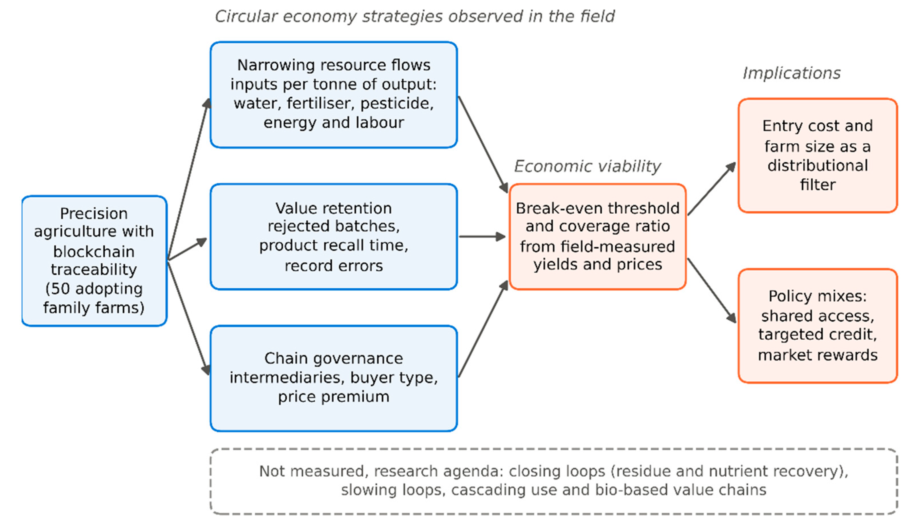
Figure 2.
Input intensity per tonne of output in the comparison group and the adopting group. Each small point is one participant (n = 50 per group), computed from twelve monthly records; large points and bars show the group mean and its 95% confidence interval. The percentage under each title is the relative difference between group means.
Figure 2.
Input intensity per tonne of output in the comparison group and the adopting group. Each small point is one participant (n = 50 per group), computed from twelve monthly records; large points and bars show the group mean and its 95% confidence interval. The percentage under each title is the relative difference between group means.
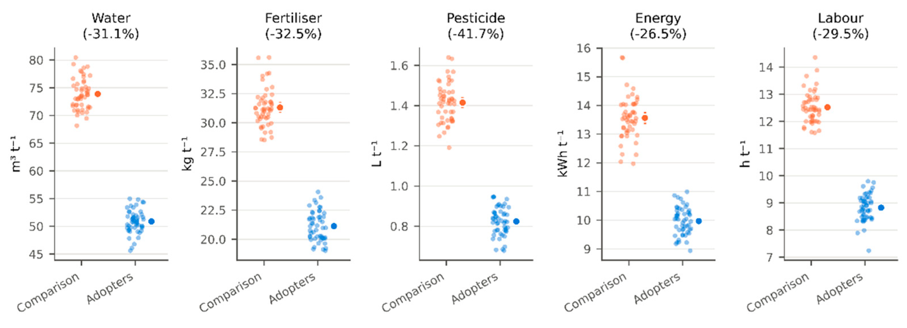
Figure 3.
Observed yield advantage against the break-even threshold, by farm. Each point is one of the 50 adopting farms at a discount rate of 12% and a five-year horizon. The horizontal axis shows the additional output each farm requires to break even, computed from its own investment, plot area and selling price; the vertical axis shows its yield advantage over the mean of the comparison group. The dashed line marks break-even and the shaded area the region of non-viability.
Figure 3.
Observed yield advantage against the break-even threshold, by farm. Each point is one of the 50 adopting farms at a discount rate of 12% and a five-year horizon. The horizontal axis shows the additional output each farm requires to break even, computed from its own investment, plot area and selling price; the vertical axis shows its yield advantage over the mean of the comparison group. The dashed line marks break-even and the shaded area the region of non-viability.
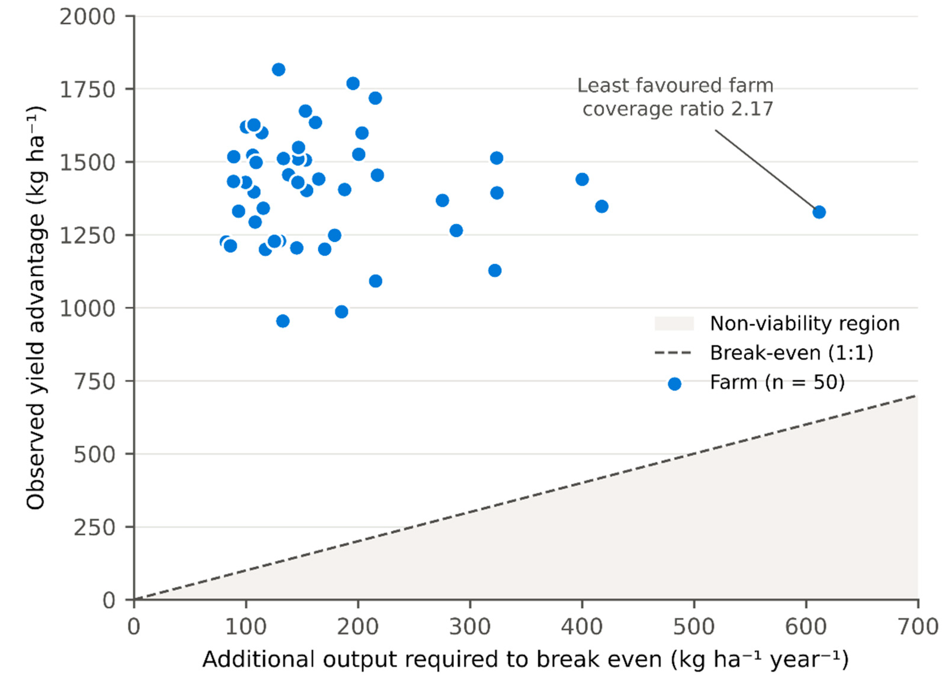
Figure 4.
Viability frontier by plot area. Points are the individual thresholds of the 50 adopting farms. Curves show the threshold implied by Equation (6) for the median recurring cost and selling price and for initial investments at the 10th, 50th and 90th percentiles of the sample. The horizontal line marks the mean observed yield differential. Discount rate 12% and five-year horizon.
Figure 4.
Viability frontier by plot area. Points are the individual thresholds of the 50 adopting farms. Curves show the threshold implied by Equation (6) for the median recurring cost and selling price and for initial investments at the 10th, 50th and 90th percentiles of the sample. The horizontal line marks the mean observed yield differential. Discount rate 12% and five-year horizon.
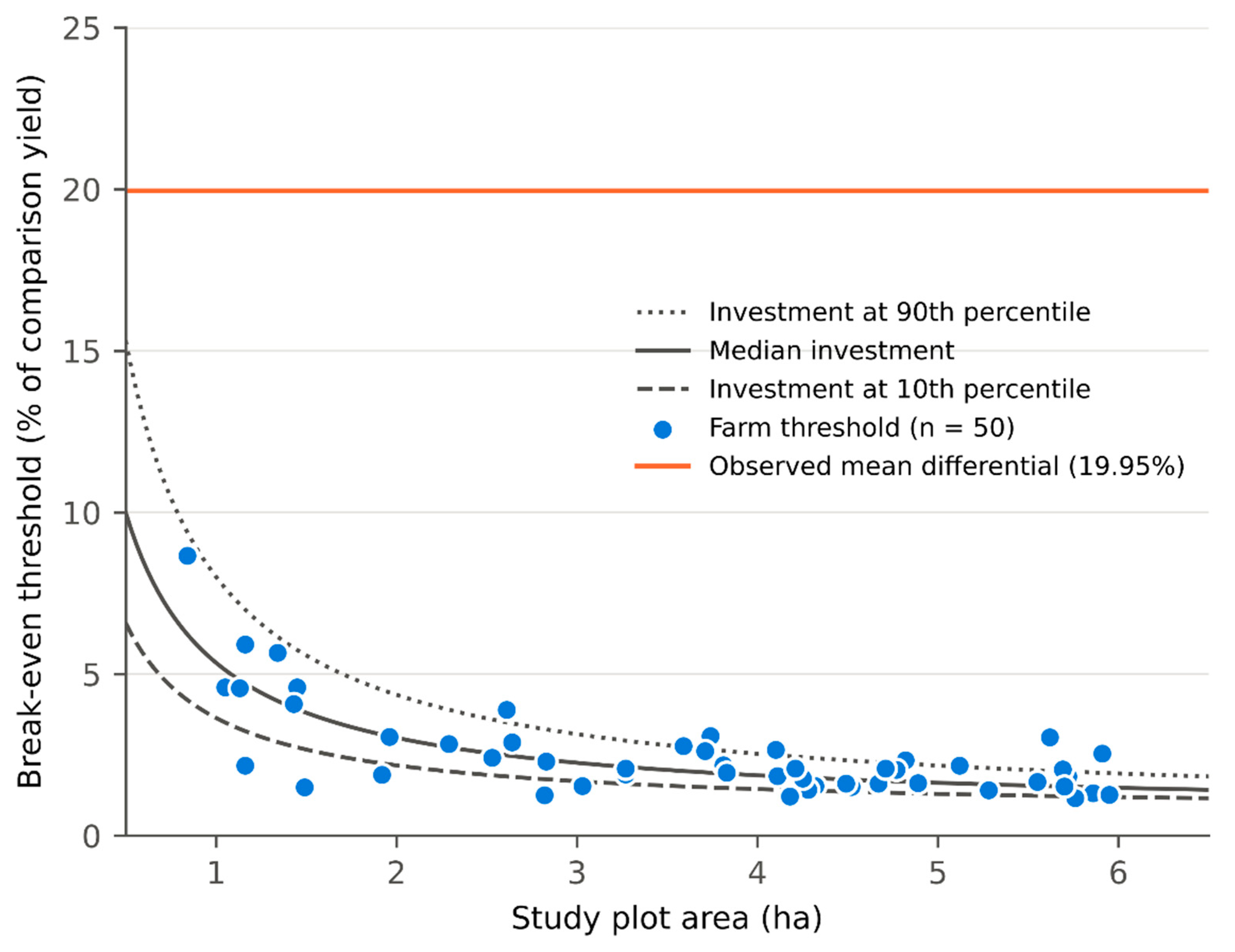
Figure 5.
Sensitivity analysis of the break-even threshold. (a) Threshold as a percentage of the comparison group yield, by evaluation horizon, for five discount rates; the circle marks the reference scenario of 12% and five years. (b) Coverage ratio by mean selling price at 12% and five years; the solid line is the mean of the 50 farms, the dashed line the least favoured farm, the horizontal line break-even and the dotted line the observed price.
Figure 5.
Sensitivity analysis of the break-even threshold. (a) Threshold as a percentage of the comparison group yield, by evaluation horizon, for five discount rates; the circle marks the reference scenario of 12% and five years. (b) Coverage ratio by mean selling price at 12% and five years; the solid line is the mean of the 50 farms, the dashed line the least favoured farm, the horizontal line break-even and the dotted line the observed price.
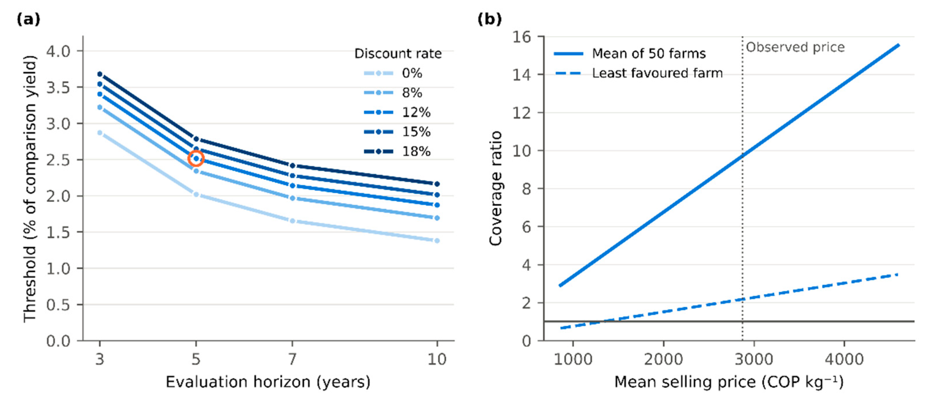
Figure 6.
Stress test of the adoption decision. Share of the 50 adopting farms that break even when only a fraction of the observed yield differential is retained, for the reference scenario and for the most and least demanding combinations of discount rate and horizon. The dotted line marks half of the observed differential.
Figure 6.
Stress test of the adoption decision. Share of the 50 adopting farms that break even when only a fraction of the observed yield differential is retained, for the reference scenario and for the most and least demanding combinations of discount rate and horizon. The dotted line marks half of the observed differential.
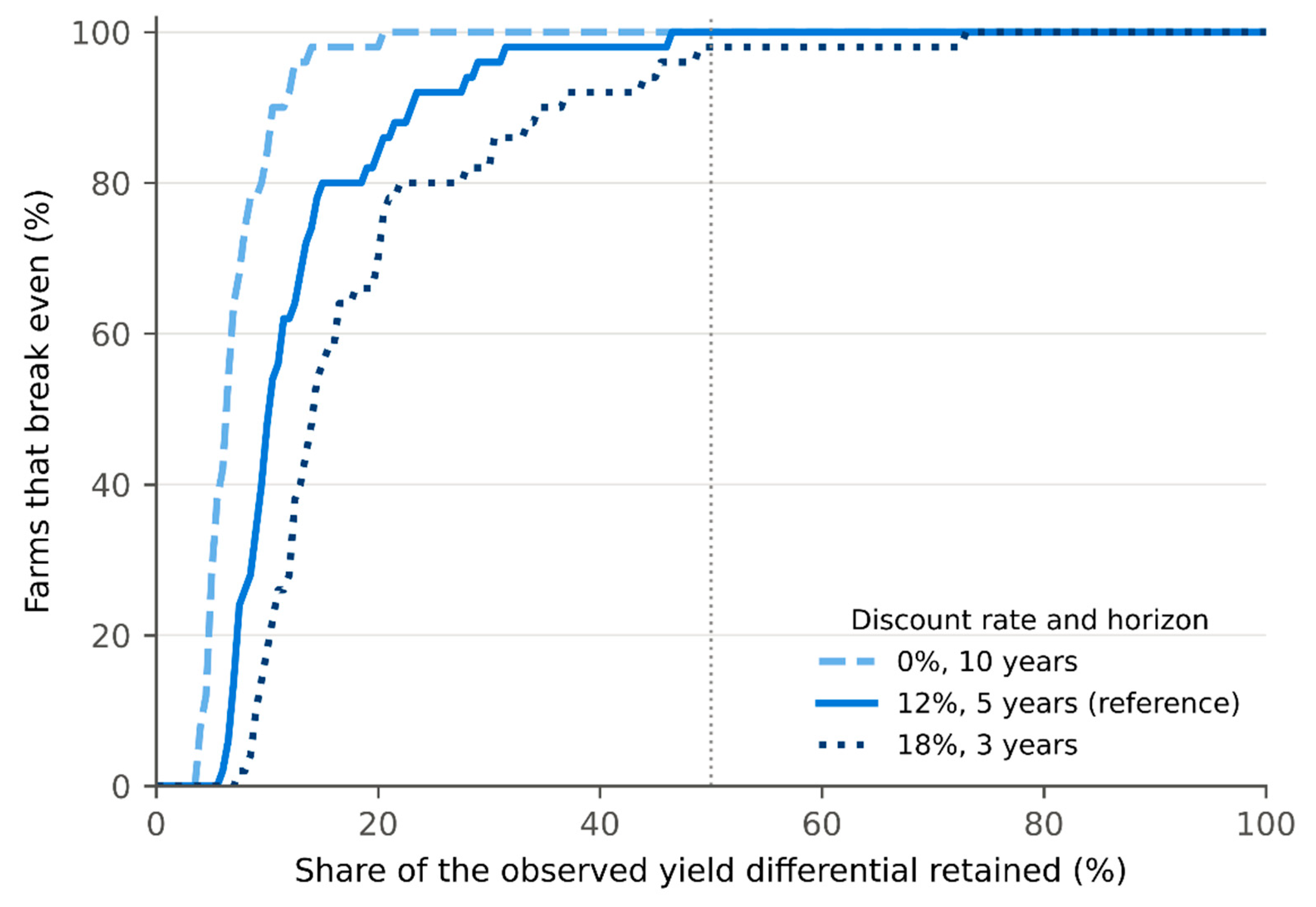
Table 1.
Model parameters for the adopting group (n = 50).
| Parameter | Mean ± SD | Median | Range | Source |
|---|---|---|---|---|
| Initial investment (COP/farm) | 3,573,096 ± 1,225,106 | 3,369,888 | 1,625,065 to 5,949,467 | Economic survey |
| Recurring cost (COP/ha/year) | 147,276 ± 35,108 | 141,895 | 82,789 to 209,915 | Economic survey |
| Selling price (COP/kg) | 2870 ± 360 | 2851 | 2162 to 3717 | Batch record |
| Study plot area (ha) | 3.67 ± 1.57 | 3.97 | 0.84 to 5.95 | Farm file |
| Discount rate (%) | n.a. | n.a. | 0 to 18 | Assumption |
| Horizon (years) | n.a. | n.a. | 3 to 10 | Assumption |
The recurring technology cost is the sum of the operating cost of the blockchain platform and equipment maintenance. SD: standard deviation; COP: Colombian pesos; n.a.: not applicable.
Table 2.
Resource efficiency and chain indicators by group (participant-level means, n = 50 per group).
Table 2.
Resource efficiency and chain indicators by group (participant-level means, n = 50 per group).
| Indicator | Adopting | Comparison | Difference (95% CI) | Change (%) | p |
|---|---|---|---|---|---|
| Input intensity per tonne of output | |||||
| Water (m3/t) | 50.89 ± 2.10 | 73.89 ± 2.80 | −23.00 (−23.98 to −22.02) | −31.1 | <0.001 |
| Fertiliser (kg/t) | 21.14 ± 1.28 | 31.32 ± 1.62 | −10.18 (−10.76 to −9.60) | −32.5 | <0.001 |
| Pesticide (L/t) | 0.82 ± 0.07 | 1.41 ± 0.10 | −0.59 (−0.62 to −0.56) | −41.7 | <0.001 |
| Energy (kWh/t) | 9.97 ± 0.48 | 13.57 ± 0.75 | −3.60 (−3.85 to −3.35) | −26.5 | <0.001 |
| Labour (h/t) | 8.83 ± 0.50 | 12.52 ± 0.58 | −3.69 (−3.91 to −3.48) | −29.5 | <0.001 |
| Value retention and chain governance | |||||
| Product traceable farm to buyer (%) | 95.79 ± 1.49 | 67.57 ± 4.66 | 28.22 (26.84 to 29.61) | 41.8 | <0.001 |
| Traceability time (h) | 1.15 ± 0.29 | 11.52 ± 2.04 | −10.36 (−10.95 to −9.78) | −90.0 | <0.001 |
| Product recall time (h) | 2.28 ± 0.54 | 22.12 ± 4.53 | −19.84 (−21.14 to −18.55) | −89.7 | <0.001 |
| Record errors per batch | 1.04 ± 0.48 | 3.97 ± 1.17 | −2.93 (−3.29 to −2.58) | −73.8 | <0.001 |
| Data discrepancies per batch | 0.55 ± 0.29 | 2.93 ± 0.79 | −2.38 (−2.62 to −2.14) | −81.1 | <0.001 |
| Rejections per batch | 0.43 ± 0.30 | 0.99 ± 0.50 | −0.55 (−0.72 to −0.39) | −56.1 | <0.001 |
| Intermediaries per batch | 1.87 ± 0.45 | 3.51 ± 0.60 | −1.64 (−1.85 to −1.43) | −46.7 | <0.001 |
| Delivery time (h) | 23.89 ± 4.62 | 24.19 ± 4.00 | −0.31 (−2.02 to 1.41) | −1.3 | 0.723 |
| Selling price (COP/kg) | 2870 ± 360 | 2961 ± 371 | −91 (−236 to 54) | −3.1 | 0.218 |
Values are mean ± SD. Differences, confidence intervals and p-values come from Welch’s t-test at participant level. Input intensity is the sum of twelve monthly input values per hectare divided by the sum of twelve monthly yields per hectare. Chain indicators are means of three batches per participant.
Table 3.
Break-even threshold by discount rate and horizon (% of the comparison group yield).
| Discount rate (%) | 3 years | 5 years | 7 years | 10 years |
|---|---|---|---|---|
| 0 | 2.87 | 2.02 | 1.65 | 1.38 |
| 8 | 3.22 | 2.34 | 1.97 | 1.69 |
| 12 | 3.40 | 2.51 | 2.14 | 1.87 |
| 15 | 3.54 | 2.65 | 2.28 | 2.01 |
| 18 | 3.68 | 2.79 | 2.42 | 2.16 |
Each cell is the mean of the thresholds computed individually for the 50 adopting farms.
Table 4.
Coverage ratio by selling price.
| Price scenario | Price (COP/kg) | Mean coverage | Minimum coverage | Viable farms |
|---|---|---|---|---|
| −50% | 1435 | 4.85 | 1.09 | 50/50 |
| −25% | 2153 | 7.28 | 1.63 | 50/50 |
| Observed | 2870 | 9.70 | 2.17 | 50/50 |
| +25% | 3588 | 12.13 | 2.71 | 50/50 |
| +50% | 4306 | 14.55 | 3.26 | 50/50 |
Discount rate 12% and five-year horizon. The coverage ratio is the quotient of the observed yield advantage and the break-even threshold, and a farm is viable when it exceeds one.
Table 5.
Threshold and coverage ratio by main crop.
| Crop | n | Threshold (%) | Coverage ratio |
|---|---|---|---|
| Leafy vegetables | 12 | 2.09 | 11.75 |
| Onion | 13 | 2.51 | 9.37 |
| Potato | 11 | 2.60 | 8.78 |
| Pea | 14 | 2.82 | 8.98 |
Discount rate 12% and five-year horizon. Threshold expressed as a percentage of the comparison group yield.
Table 6.
Positioning of this study within recent evidence on digital technologies, circular economy and bioeconomy.
Table 6.
Positioning of this study within recent evidence on digital technologies, circular economy and bioeconomy.
| Study | Focus and method | Main finding | What remains open |
|---|---|---|---|
| Kouhizadeh et al. [19] | Blockchain and circular economy; multiple case studies across sectors | Early evidence linking blockchain applications to circular economy dimensions, with tensions in practice | Farm-level economics and smallholder settings |
| Böhmecke-Schwafert et al. [21] | Blockchain innovations for the circular economy; expert interviews | Blockchain plays a moderating role and is seen as infrastructure rather than a panacea | Measured outcomes in agri-food chains |
| Rejeb et al. [22] | Systematic review of 70 articles on blockchain and the circular economy | Six research themes, including sector applications and adoption barriers | Empirical evaluations with field data |
| Velasco-Muñoz et al. [2] | Circular economy in agriculture; review and indicator assessment | Definition and strategies for agricultural circularity and an assessment of 41 indicators | Application of indicators to digital interventions |
| Lan and Ban [28] | Precision agriculture; global meta-analysis | Farm-level economic and environmental benefits, weaker on small farms and in developing countries | Decision rules for small farms |
| Grilli et al. [54] | Bioeconomy investment in Colombia; decision support procedure | Formal assessment combining national indicators, regional features and stakeholder views | Farm-level viability of digital tools |
| This study | Precision agriculture with blockchain; quasi-experiment with 100 family farms and threshold model | Inputs per tonne 26 to 42% lower, fewer rejections, threshold of 2.51% met by all farms, viability governed by entry cost | Closing loops, causal identification, market rewards |
Table 7.
Research agenda by circular economy and bioeconomy strategy.
| Strategy | Status in this study | Pending question | Data required | References |
|---|---|---|---|---|
| Narrowing resource flows | Measured (association) | Causal size of input reductions per tonne | Randomised or staggered rollout; purchase records | [2,18] |
| Separate contribution of each technology | Not separable (combined package) | Effects of precision agriculture and traceability on their own | Factorial or staggered rollout | [30,32] |
| Value retention and food loss | Partly measured | Physical and economic value of avoided losses | Rejected quantities and their destination | [59,60] |
| Closing loops | Not measured | Recovery of crop residues and nutrients on pea, potato, onion and vegetable farms | Residue flows, composting and nutrient balances | [3,68] |
| Slowing loops and access models | Not measured | Effect of shared or service-based equipment on thresholds | Costs and use of shared equipment | [18,62] |
| Cascading use and bio-based value chains | Not measured | Place of family farms in regional bioeconomy chains | Regional input-output and value chain data | [4,54] |
| Governance and inclusion | Inferred from thresholds | Policy mixes that widen participation of small farms | Programme design and uptake by farm size | [45,46,63] |
| Market rewards for verified origin | Measured (no premium) | Conditions under which traceability earns a premium | Prices across channels and certification | [64,65,66] |
| Regenerative outcomes | Not measured | Effects on soil health and ecosystem services | Soil indicators over several seasons | [69] |
Disclaimer/Publisher’s Note: The statements, opinions and data contained in all publications are solely those of the individual author(s) and contributor(s) and not of MDPI and/or the editor(s). MDPI and/or the editor(s) disclaim responsibility for any injury to people or property resulting from any ideas, methods, instructions or products referred to in the content. |
© 2026 by the authors. Licensee MDPI, Basel, Switzerland. This article is an open access article distributed under the terms and conditions of the Creative Commons Attribution (CC BY) license (http://creativecommons.org/licenses/by/4.0/).
Copyright: This open access article is published under a Creative Commons CC BY 4.0 license, which permit the free download, distribution, and reuse, provided that the author and preprint are cited in any reuse.