

Submitted:
15 November 2026
Posted:
17 November 2026
You are already at the latest version
Abstract
Should a central bank still look through energy price shocks when inflation is already high? We address the question with state-dependent local projections on a monthly panel of the twenty euro area countries from 2001 to 2025, using innovations in euro-denominated oil and natural gas prices. A price-setting framework with state-dependent price adjustment, real wage resistance and limited attention delivers three testable predictions. The evidence supports the look-through prin- ciple in three respects. Average second-round effects are small: a 10 per cent oil price innovation raises core prices by 0.13 per cent after one year. Beyond the month of the shock, transmission from commodity prices to consumer energy prices does not depend on the inflation regime. Out- side two episodes, pass-through to core prices when inflation exceeds 4 per cent is no larger than at low inflation. State dependence is present in household expectations, which respond immedi- ately to gas price innovations only when inflation is high, a result that holds when any single year is excluded. In the full sample, oil pass-through to core prices is 0.31 per cent in the high-inflation regime against 0.07 per cent otherwise, and we show that this difference originates in 2008 and 2022, when energy prices moved together with large aggregate disturbances. Gas shocks transmit more slowly and more persistently than oil shocks. The results indicate that the case for respond- ing more forcefully to energy shocks at high inflation rests on expectations and on the coincidence of shocks, and less on a mechanical rise in pass-through.
Keywords:
inflation
; energy prices
; pass-through
; state dependence
; inflation expectations
; local projections
; euro area
1. Introduction
The standard prescription for monetary policy after an energy price shock is to look through its direct effect on headline inflation and to respond only to second-round effects on wages, core prices and expectations (Bernanke et al., 1997; Clarida et al., 1999; Blanchard and Galí, 2007a). The prescription rests on an empirical premise, that second-round effects are small, and for two decades before 2021 the premise held (Blanchard and Galí, 2007b).
The inflation surge of 2021–2023 raised the question of whether the premise is conditional. Euro area headline inflation peaked at 10.6 per cent in October 2022, and core inflation reached its highest level since the start of monetary union. Theory gives reasons to expect stronger pass-through at high inflation. In menu-cost models the frequency of price adjustment rises with inflation, so cost shocks reach prices faster (Golosov and Lucas, 2007; Alvarez et al., 2019; Cavallo et al., 2024). Taylor (2000) argued that low inflation itself lowers pass-through. Workers resist real wage losses more when inflation is high and visible (Blanchard and Galí, 2007a). Households and firms attend to inflation once it crosses a threshold (Sims, 2003; Maćkowiak and Wiederholt, 2009; Pfäuti, 2026). If these mechanisms are strong, looking through is appropriate at low inflation and costly at high inflation, a conditionality that Guerrieri et al. (2023) emphasise.
This paper tests the conditionality directly. We ask three research questions.
- How large is the pass-through of oil and natural gas price innovations to consumer energy prices, core prices and household inflation expectations in the euro area?
- Is that pass-through stronger when inflation is already high, and at which stage of transmission?
- Is pass-through lower where fiscal policy shielded households and firms from energy prices?
To answer them we estimate state-dependent local projections (Jordà, 2005; Auerbach and Gorodnichenko, 2012; Ramey and Zubairy, 2018) on a monthly panel of the twenty euro area countries from July 2001 to December 2025. The impulses are innovations in the euro prices of Brent crude oil and European natural gas. The state is whether a country’s headline inflation exceeded 4 per cent in the previous month. Because national inflation rates differ inside the monetary union, the regime varies across countries at a given date. We exploit this in a specification with time fixed effects, which removes all common shocks. Section 2 derives the predictions that the estimates test.
The answers are as follows. On the first question, average second-round effects are small and estimated with precision. A 10 per cent oil price innovation raises consumer energy prices by 2.5 per cent and core prices by 0.13 per cent after one year. Gas price innovations transmit more slowly and more persistently: core prices rise by 0.12 per cent after one year and by 0.24 per cent after two.
On the second question, the evidence is favourable to the look-through principle on two counts and identifies state dependence on a third. Beyond the month of the shock, transmission from commodity prices to consumer energy prices is the same in both regimes. For core prices, the full-sample estimates show amplification for oil, with a response of 0.31 per cent after one year at high inflation against 0.07 per cent at low inflation. This difference is specific to two years. Excluding the impulses of either 2008 or 2022 reduces it to about 0.1 and removes its statistical significance, and in the sample that ends in 2020 the two regimes are indistinguishable. Outside these episodes, a high inflation rate has not by itself been associated with stronger pass-through to core prices. State dependence does appear in household expectations. On impact, expectations respond to gas price innovations only in the high-inflation regime. This result holds when any single year is excluded and in the sample that ends before the recent surge.
On the third question, countries that committed more fiscal resources to energy support in 2021–2023 do not show systematically lower pass-through.
The paper makes three contributions. The first is a set of pass-through estimates for oil and gas on a common panel, in euro, that covers the full 2021–2023 episode and its aftermath. The second is a decomposition of state dependence by stage of transmission, which locates it in expectations and not in retail energy pricing. The third is methodological. We show that the standard robustness checks for state-dependent local projections, such as alternative thresholds and transition functions, leave the identifying episodes unchanged, and we propose two diagnostics that reveal them: leave-one-year-out estimates and the share of regime-specific identifying variation contributed by each year.
For policy, the results support looking through energy shocks as a baseline and indicate where vigilance is warranted. The risk at high inflation comes from the immediate reaction of expectations and from the coincidence of energy shocks with other large disturbances. A mechanical increase in cost pass-through at high inflation is not established by the data.
The paper relates to three literatures. The first measures the macroeconomic effects of energy shocks (Hamilton, 1983; Kilian, 2009; Baumeister and Hamilton, 2019; Känzig, 2021) and their role in the recent inflation (Gagliardone and Gertler, 2026; Bernanke and Blanchard, 2025; Ball et al., 2022). Adolfsen et al. (2024) study gas price shocks and euro area inflation, and De Santis and Tornese (2025) document non-linear effects of energy supply shocks. We add a cross-country panel design and an account of which episodes identify the non-linearity. The second literature concerns non-linear inflation dynamics and the Phillips curve (Benigno and Eggertsson, 2023; Hazell et al., 2022; McLeay et al., 2020). Our time fixed effects specification applies the logic of regional identification to pass-through. The third concerns expectations formation and attention (Coibion and Gorodnichenko, 2015; D’Acunto et al., 2021; Weber et al., 2022; Reis, 2022).
2. Conceptual Framework
This section derives the pass-through of an energy price change to core prices in a standard New Keynesian setting and states the conditions under which it depends on the level of inflation. All variables are log deviations from a steady state.
2.1. Price Setting and Marginal Cost
Firms in the core sector set prices as in Calvo (1983). A fraction of firms resets its price each period. Core inflation follows the New Keynesian Phillips curve (Clarida et al., 1999; Galí and Gertler, 1999)
where is the discount factor and is real marginal cost. The slope is decreasing in : the more often prices are reset, the more strongly inflation responds to costs.
Production uses energy and labour. Let denote the price of energy relative to core prices and the real product wage. With an energy cost share ,
An energy price increase lowers the consumption real wage in proportion to the share of energy in consumption, . Following the treatment of real wage rigidity in Blanchard and Galí (2007a), workers recover a fraction of that loss through higher wages, and wages also respond to economic activity :
The parameter measures real wage resistance. With workers absorb the terms-of-trade loss and energy affects marginal cost only directly. Substituting (3) into (2) gives
The first component of is the direct cost channel. The second is the second-round effect through wages.
2.2. Pass-Through to Core Prices
Let the relative price of energy follow with , where is an energy price innovation. Holding activity fixed and solving (1) forward gives . To first order, the response of the core price level at horizon h to a unit innovation is
Pass-through rises with the frequency of price adjustment, since , and with real wage resistance, since .
Pass-through is state-dependent if these parameters vary with inflation. In models with a fixed cost of price adjustment, the frequency of adjustment increases with trend inflation (Golosov and Lucas, 2007; Alvarez et al., 2019), so with . Wage indexation and bargaining over real wages gain importance when inflation is high, so with . Both imply
2.3. Retail Energy Prices
Consumer energy prices are among the most flexible prices in the consumption basket. Let be the consumer energy price and the commodity price. With flexible pricing, , where reflects the share of the commodity in the retail price after refining, distribution, network charges and specific taxes. Under this pricing rule does not depend on or . The first stage of transmission is then independent of the inflation regime.
2.4. Expectations and Attention
Households form expectations with limited attention (Sims, 2003; Maćkowiak and Wiederholt, 2009). Let be the household expectation of inflation,
where is a signal that loads on salient prices, of which energy is the leading example (D’Acunto et al., 2021), and is the weight on new information. Under an attention threshold, is higher when inflation exceeds the threshold (Pfäuti, 2026). The impact response of expectations to an energy price innovation is proportional to , so it is larger at high inflation.
2.5. Testable Predictions and a Caveat
The framework delivers three predictions for the regime-specific responses estimated below.
- P1 (core prices). The response of core prices to an energy price innovation is larger in the high-inflation regime, by (6).
- P2 (retail energy). The response of consumer energy prices does not differ across regimes.
- P3 (expectations). The impact response of household expectations is larger in the high-inflation regime, by (7).
Together, P1 and P2 locate state dependence after the retail energy stage.
Equation (4) also contains a caveat for measurement. The derivation of holds activity fixed. If, within a regime, energy price innovations are correlated with the path of activity, a regression of core prices on the innovation recovers
which exceeds when energy prices and activity move together. The second term matters most when a regime is populated by few episodes, because the covariance does not average out. The empirical analysis therefore asks two things of the data: whether the regime-specific responses differ, and whether the difference is a property of the regime or of particular episodes.
3. Data
The panel covers the twenty countries that formed the euro area from 2023 to 2025.1 All series are monthly. Appendix A lists sources and series codes.
Prices. We use the Harmonised Index of Consumer Prices (HICP) from Eurostat, 2015 = 100, not seasonally adjusted, for all items, for energy, and for all items excluding energy, food, alcohol and tobacco. We refer to the last as core. The indices end in December 2025.
Expectations. Household price expectations come from the Joint Harmonised EU Programme of Business and Consumer Surveys of the European Commission. Question 6 asks how consumer prices will develop over the next twelve months. We use the seasonally adjusted balance statistic, which rises when more respondents expect prices to increase faster.
Energy commodity prices. Brent crude oil and European natural gas prices are monthly averages from the World Bank Commodity Price Data. We convert them from US dollars to euro with the monthly average reference exchange rate of the European Central Bank, so that the impulses measure the price faced by euro area importers. The European gas series is the Title Transfer Facility price in the recent sample and an average import border price in earlier years, so its early variation partly reflects oil-indexed contracts.
Controls. The unemployment rate is the seasonally adjusted Eurostat series. Global supply conditions are measured by the Global Supply Chain Pressure Index of Benigno et al. (2022).
Fiscal support. The Bruegel dataset of Sgaravatti et al. (2023) records the national measures adopted between September 2021 and January 2023 to shield households and firms from high energy prices. We use the total allocated amount, scaled by 2022 nominal GDP. Support ranges from 0.5 per cent of GDP in Finland to 5.5 per cent in Malta.
Oil supply news. For a validation exercise we use the oil supply news surprises of Känzig (2021), which are available to December 2017.
Table 1 reports descriptive statistics for the estimation sample, July 2001 to December 2025. Figure 1 shows the two commodity prices and the share of countries with inflation above 4 per cent. High inflation is concentrated in two periods. Of the 956 country-months in the high-inflation regime, 16.3 per cent of the sample, 177 fall in 2007–2009 and 440 in 2021–2023. Appendix Table A2 gives the distribution by country.
4. Empirical Methodology
4.1. Energy Price Innovations
Let be 100 times the log euro price of commodity , for oil and gas. The innovation is the residual of the forecasting regression
where contains euro area twelve-month inflation, the euro area unemployment rate and the Global Supply Chain Pressure Index. By construction is orthogonal to past energy prices and to the lagged state of the euro area economy. The innovations have standard deviations of 8.2 per cent for oil and 9.8 per cent for gas, are serially uncorrelated, and have a mutual correlation of 0.09. Regression (9) explains 18 per cent of the variance of oil price changes and 31 per cent for gas.
The innovations are reduced-form. They combine news about global supply and global demand (Kilian, 2009). The estimand is therefore the average response to an unanticipated change in the euro price of energy, which is the object that a policy of looking through energy prices takes as given. Section 6 uses the instrument of Känzig (2021) to assess a supply interpretation.
4.2. State-Dependent Local Projections
Let denote 100 times the log of a price index, or the survey balance, in country and month . Let indicate the high-inflation regime, where is twelve-month headline inflation and per cent, twice the inflation target of the European Central Bank. For each horizon we estimate by least squares
The coefficient is the cumulative response at horizon h in regime , the empirical counterpart of in (5) for core prices. Predictions P1 and P3 state that for core prices and, at , for expectations. Prediction P2 states that for consumer energy prices. We test these with the difference . A linear benchmark imposes .
The fixed effects vary by country and calendar month . They absorb country effects and the country-specific seasonal pattern of the unadjusted indices. The vector contains six lags of , lagged headline inflation, the lagged unemployment rate, the lagged Global Supply Chain Pressure Index and three lags of each innovation. All controls have regime-specific coefficients, as in Ramey and Zubairy (2018).
Three assumptions give (10) a causal interpretation as the response to an energy price innovation.
- A1 (unanticipated impulse). For all , . The innovation is unforecastable given the controls.
- A2 (predetermined state). is determined before . The response is conditional on the regime at the time of the shock and incorporates the average transition between regimes afterwards (Gonçalves et al., 2024).
- A3 (comparable impulses). The joint distribution of the innovation and other contemporaneous shocks is the same in both regimes.
Assumptions A1 and A2 hold by construction of the innovation and by timing. Assumption A3 is what allows to be read as an effect of the regime. It fails if energy innovations in the high-inflation regime coincide with other disturbances, which is the case described by (8). Section 4.4 and Section 4.5 set out how we examine it. Local projections estimate the same impulse responses as vector autoregressions in population and remain valid under the persistence of the data when lags of the dependent variable are included (Plagborg-Møller and Wolf, 2021; Montiel Olea and Plagborg-Møller, 2021).
4.3. Inference
The innovations are common to all countries, so is correlated across i, and it is serially correlated for by construction of the long difference. Let collect the regressors of (10) after partialling out the fixed effects and let . We use the covariance estimator of Driscoll and Kraay (1998),
where and
The estimator is robust to arbitrary cross-sectional dependence, to heteroskedasticity and to serial correlation up to the bandwidth . Tests use the t distribution with degrees of freedom. Responses are reported per 10 per cent innovation.
4.4. Identification from Cross-Country Differences
Because differs across countries in the same month, we can add month fixed effects :
The month effects absorb the innovations, the common monetary policy stance and every other euro area-wide disturbance. The difference is then identified only by comparing, within a month, countries in the high-inflation regime with countries in the low-inflation regime. Assumption A3 is replaced by the weaker requirement that country-specific shocks are unrelated to the interaction of the common innovation with the national regime. This is the pass-through analogue of the regional identification of the Phillips curve in Hazell et al. (2022) and McLeay et al. (2020).
4.5. Episode Diagnostics
High-inflation observations are clustered in time, so a regime-specific coefficient may be identified by few episodes. Two diagnostics make this visible.
The first is the share of regime-specific identifying variation contributed by calendar year a,
which measures how much of the variation that identifies comes from each year.
The second is the leave-one-year-out estimate , obtained by re-estimating (10) without the impulses dated in year a. If is a property of the regime, the estimates should be stable across a. Sensitivity to a single year indicates that the difference is specific to that episode. These diagnostics complement the usual variations of threshold, transition function and lag length, which change the specification but not the episodes that identify it.
5. Results
5.1. Average Pass-Through
Table 2 and Figure 2 report the linear responses. A 10 per cent oil price innovation raises consumer energy prices by 0.96 per cent within the month and by 2.5 per cent after one year. Headline prices rise by 0.45 per cent after one year. Core prices respond slowly and little: 0.08 per cent after six months and 0.13 per cent after one year, with a standard error of 0.05. The price expectations balance rises by 0.7 points on impact and by 2.6 points after six months, and the effect fades within two years.
Gas price innovations transmit differently. The response of consumer energy prices builds gradually to about 1 per cent after two years and is imprecisely estimated, which is consistent with long-term contracts and regulated retail tariffs. The response of core prices is 0.12 per cent after one year and 0.24 per cent after two, and both are significant at the 5 per cent level. Expectations do not respond significantly at any horizon in the linear specification.
These estimates answer the first research question. Second-round effects on core prices are an order of magnitude smaller than the direct effect on energy prices. For gas they continue to build in the second year.
5.2. Pass-Through by Inflation Regime
Retail energy (P2). The response of consumer energy prices to oil is 2.2 per cent in the high regime and 2.6 per cent in the low regime after one year. The difference changes sign across horizons and is insignificant at the 5 per cent level at every horizon reported in Table 3. For gas, the impact response is larger in the high regime, 0.30 against 0.06 per cent (), and the difference is insignificant at later horizons. Prediction P2 is broadly supported: beyond the month of the shock, the first stage of transmission does not depend on the inflation regime.
Core prices (P1). For oil, the response after one year is 0.31 per cent (standard error 0.11) in the high regime and 0.07 per cent (0.04) in the low regime. The difference of 0.24 percentage points has a p-value of 0.023. After two years the responses are 0.33 and 0.02 per cent (). In the full sample the oil estimates agree with P1. For gas they do not. The response is larger in the low regime at long horizons, 0.36 per cent against per cent after two years ().
Expectations (P3). On impact the balance rises by 2.0 points in the high regime and 0.4 points in the low regime after an oil innovation (), and by 1.1 points against points after a gas innovation (). The differences fade within a year. Prediction P3 is supported for both commodities.
Taken together, the full-sample estimates locate state dependence after the retail energy stage, as the framework predicts, with one exception: the sign of the gas result for core prices. Section 6 examines whether the differences are properties of the regime.
6. Regime or Episode?
6.1. Specification Choices
Table 4 reports for four statistics: core prices after twelve months and expectations on impact, each for oil and gas. The first block varies the specification. Thresholds of 3 and 5 per cent, a logistic transition function, a regime defined on core inflation, and twelve lags of the dependent variable leave the oil result for core prices between 0.18 and 0.33 percentage points, always significant at the 5 per cent level. The impact response of expectations to gas is between 0.71 and 1.36 points. Excluding the Baltic countries, which account for a large share of pre-2021 high-inflation observations, or the first months of the pandemic, changes little. By these conventional checks the results are robust.
6.2. Which Episodes Identify the Difference
The diagnostics of Section 4.5 give a different picture for core prices. By the measure in (13), 25 per cent of the high-regime identifying variation for oil comes from 2008 and 24 per cent from 2022. For gas, 91 per cent comes from 2021–2023.
Figure 4 shows the leave-one-year-out estimates. For oil and core prices, 23 of the 25 estimates lie between 0.19 and 0.37 and are significant at the 10 per cent level. The two exceptions are the exclusion of 2008, which gives 0.12 (), and the exclusion of 2022, which gives 0.10 (). Table 4 confirms the pattern. When impulses dated July 2008 to June 2009 are excluded, the difference is with a standard error of 0.17, and the regime-specific responses are 0.04 per cent at high inflation and 0.06 per cent at low inflation. In the sample that ends in December 2020 the difference is also .
The two episodes share a feature. Between July and December 2008 the euro price of oil fell by almost two thirds. Until October, inflation was still above 4 per cent in at least half of the countries. Core inflation then declined through 2009, in the deepest recession of the sample. In 2022 oil prices rose sharply after the invasion of Ukraine, while supply bottlenecks and the reopening of the economy were already raising core inflation. In both cases the energy innovation and the path of activity moved together, which is the condition under which (8) overstates . The gas result has the same structure with the opposite sign. The large gas innovations of September and October 2021 arrived when 17 of the 20 countries were still classified in the low regime, and were followed by the rise in core inflation of 2022. Innovations in 2022 arrived in the high regime and were followed by disinflation as energy prices reversed and policy tightened.
The positive reading of this evidence is that the high-inflation observations outside the two episodes, which include the Baltic and central European inflations of the 2000s, show pass-through to core prices that is as low as in the low-inflation regime. Amplification occurred in the episodes in which an energy shock coincided with other large disturbances.
6.3. Expectations
The expectations results separate by commodity. For oil, the larger impact response in the high regime depends on 2022: excluding that year reduces the difference from 1.59 to 0.11 points, and in the sample to 2020 it is 0.09.
For gas, the result is stable. The leave-one-year-out estimates range from 0.52 to 1.52 points, and all 25 are significant at the 10 per cent level. The smallest, from the exclusion of 2022, has a p-value of 0.057. In the sample that ends in 2020 the difference is 1.67 points (), so the result is present before the recent surge. Excluding the 2008–2009 crisis year gives 1.37 points (). Among the differences examined in this paper, this is the one that passes the episode diagnostics, and it is the one that prediction P3 concerns.
6.4. Cross-Country Identification
Specification (12) removes all common shocks. The estimated difference for oil and core prices after twelve months is 0.16 percentage points with a standard error of 0.14 (). The sign agrees with the baseline, the magnitude is about two thirds of it, and zero cannot be rejected. For gas the difference is and insignificant. Figure 5 shows the full horizon profiles.
For expectations, the differences with time fixed effects are points for oil and 0.28 points for gas, and neither is significant. The stronger reaction of expectations to gas at high inflation is therefore a time-series result. Expectations in all countries reacted immediately to gas prices in periods when inflation was high in many of them, and countries with higher inflation did not react more than others at the same date. This suggests that the relevant state for attention is common to the euro area, which is plausible when news about energy prices and inflation is shared across countries.
6.5. Inflation or Slack?
The last row of Table 4 replaces the inflation regime with a labour market regime, defined as an unemployment rate below the country’s sample median. Oil pass-through to core prices is 0.16 percentage points larger when the labour market is tight (). In terms of the framework, this is consistent with a role for in (4): cost shocks pass through more when activity is strong. It connects the question to the non-linear Phillips curve of Benigno and Eggertsson (2023) and suggests that the state that matters for pass-through may be slack as much as the level of inflation.
6.6. Oil Supply News
To assess a supply interpretation, we instrument the monthly log change of the oil price with the oil supply news surprises of Känzig (2021) over July 2001 to December 2017 in the linear specification (Stock and Watson, 2018). The instrument is weak in this sample, with a heteroskedasticity-robust first-stage F statistic of 7.9. The estimated response of consumer energy prices after twelve months is 5.8 per cent per 10 per cent oil price change (standard error 3.6), against 3.1 per cent (0.4) for the innovation over the same sample. The response of core prices is 0.01 per cent (0.28) against 0.11 per cent (0.06). The instrumental variable estimates do not contradict the reduced-form estimates and are too imprecise to add to them. The instrument does not cover 2021–2023, so a state-dependent version is not feasible.
7. Fiscal Energy Support
Governments spent large sums in 2021–2023 to limit the effect of energy prices on households and firms. To answer the third research question, we estimate a version of (12) in which each innovation is interacted with standardised fiscal support as a share of GDP, separately for impulses dated September 2021 to June 2023 and for all other months. The second interaction is a placebo, because support could not affect pass-through before it existed.
Table 5 reports the results. For consumer energy prices, oil pass-through in the support period is lower in countries with more support, with a coefficient of at three months. The placebo coefficient for other months is also negative and significant, at , which indicates that part of the difference reflects permanent features of retail energy pricing in these countries. The coefficients for gas are positive and insignificant. For core prices the coefficients in the support period are small and of opposite sign for oil and gas. Figure 6 gives the cross-sectional view. The cumulative change in energy prices between August 2021 and December 2022 is unrelated to the size of support: the slope is per percentage point of GDP with a robust standard error of 2.6. For core prices the slope is with a standard error of 0.6.
The cross-country data therefore do not reveal an effect of the size of support on pass-through. This does not show that the measures were ineffective. Support was not randomly assigned, and countries more exposed to gas adopted larger packages, which biases the comparison against finding lower pass-through. Packages also differed in composition, and income transfers do not act on prices directly. With twenty countries the design has limited power. Evidence at the level of individual measures and households, as in Pallotti et al. (2024), is better suited to the question.
8. Discussion
8.1. What the Evidence Supports
Three results are positive and stable. Average second-round effects of energy prices on core prices are small. The transmission of commodity prices to consumer energy prices is independent of the inflation regime. Household expectations react immediately to gas prices when inflation is high. The first two support the look-through principle. The third identifies the channel through which high inflation changes the transmission of energy shocks.
For core prices, the mechanism in (6) is neither confirmed nor excluded as a general property. The estimates agree with it in the two episodes that dominate the high-inflation regime and show no amplification elsewhere. Confidence intervals outside those episodes are wide. With the 2008–2009 crisis year excluded, the 90 per cent interval for the oil difference runs from to percentage points, so amplification of the baseline magnitude cannot be ruled out. The appropriate conclusion is conditional: amplification has been observed when energy shocks coincided with other large disturbances, and has not been observed in their absence.
8.2. Implications for Monetary Policy
The results bear on the design of the policy response in three ways.
First, looking through energy shocks remains a sound baseline. A 10 per cent oil price increase adds about 0.1 per cent to the core price level after a year. For gas the effect is of similar size at one year and roughly doubles in the second year, which a policy horizon of one to two years captures only in part. Gas shocks call for a longer horizon of assessment than oil shocks.
Second, the case for a more forceful response at high inflation is best made through expectations. The immediate reaction of expectations to gas prices at high inflation is the stable form of state dependence in the data, and it is consistent with attention thresholds (Pfäuti, 2026). Its duration is short, less than six months, which points to heightened attention to salient prices (D’Acunto et al., 2021) more than to a lasting de-anchoring. Communication during energy price increases at high inflation addresses the channel that the data identify.
Third, what makes an energy shock at high inflation dangerous in the historical record is its coincidence with other shocks and with tight labour markets. This favours a response conditioned on the state of demand and of the labour market, in line with Benigno and Eggertsson (2023), over a rule conditioned on the inflation rate alone. A risk-management argument for acting more forcefully at high inflation remains valid, because the cost of underestimating second-round effects is larger when expectations are attentive (Reis, 2022). That argument rests on the asymmetry of risks.
8.3. Implications for Research
Evidence on state-dependent inflation dynamics from the post-2020 period faces a common difficulty. Regime indicators based on inflation or labour market tightness take the value one in a small number of adjacent months, in which several large shocks occurred. Alternative thresholds, transition functions and lag lengths do not address this, because they leave the identifying episodes unchanged. In our application every such check confirmed the baseline, and the two diagnostics of Section 4.5 changed its interpretation. Both are simple to compute, and we suggest that studies of state dependence report them.
Cross-sectional identification offers a way forward. Within the euro area, national inflation rates in October 2022 ranged from about 7 to above 20 per cent. Our time fixed effects estimates use this variation and are imprecise at the country level. Regional and sectoral price data and firm-level data on price adjustment provide many more units and would raise power (Gagliardone and Gertler, 2026; Hazell et al., 2022).
8.4. Limitations
Three limitations qualify the results. The innovations are reduced-form and combine supply and demand disturbances; the available supply instrument is weak in this sample and ends in 2017. The European gas price series changes definition over the sample, and almost all of its high-regime variation is recent, so the gas results for core prices describe one episode. The survey measure of expectations is qualitative, and a change in the balance cannot be mapped into percentage points of expected inflation.
9. Conclusion
This paper asked whether the pass-through of energy price shocks is stronger when inflation is high, using a monthly panel of euro area countries over 25 years and a framework that distinguishes three stages of transmission. Average pass-through to core prices is small, and transmission to consumer energy prices does not depend on the inflation regime. Household expectations respond immediately to gas prices when inflation is high, and this result is stable across subsamples. Stronger pass-through of oil prices to core prices at high inflation is found in the full sample and traced to 2008 and 2022, two years in which energy prices moved with other large disturbances. Gas shocks transmit more slowly and more persistently than oil shocks, and fiscal energy support is not associated with lower pass-through across countries.
The findings support looking through energy price shocks as a baseline. They indicate that, at high inflation, policy should watch household expectations and the state of demand, which are the channels through which energy shocks have had larger effects, and they provide two diagnostics for separating regimes from episodes in future work on state-dependent inflation dynamics.
Funding
The authors declare that no financial support or funding was received from any public, commercial, or non-profit organization for the research, authorship, and/or publication of this article.
Conflicts of Interest
The authors declare no competing interests.
Funding:
All data are publicly available from the sources listed in Appendix A.
Appendix A. Data Sources

Table A1.
Data sources
| Variable | Source and series | Coverage used |
| HICP: all items, energy, all items excl. energy, food, alcohol and tobacco | Eurostat, prc_hicp_midx, index 2015 = 100; items CP00, NRG, TOT_X_NRG_FOOD | 1996M1–2025M12 |
| Unemployment rate | Eurostat, une_rt_m, seasonally adjusted, per cent of labour force | to 2025M12 |
| Gross domestic product | Eurostat, nama_10_gdp, current prices, million euro | 2022 |
| Price expectations | European Commission, Business and Consumer Surveys, consumer survey question 6, seasonally adjusted balance | to 2025M12 |
| Brent crude oil; natural gas, Europe | World Bank Commodity Price Data, monthly prices, converted to euro | 1999M1–2025M12 |
| US dollar/euro exchange rate | European Central Bank, reference rate, monthly average, EXR.M.USD.EUR.SP00.A | 1999M1–2025M12 |
| Global Supply Chain Pressure Index | Federal Reserve Bank of New York | 1998M1–2025M12 |
| Fiscal energy support | Bruegel, National fiscal policy responses to the energy crisis, version of 31 July 2023 | 2021M9–2023M1 |
| Oil supply news surprises | Replication files of Känzig (2021) | to 2017M12 |
Appendix B. Regime Observations by Country
Table A2.
High-inflation regime by country, July 2001 to December 2025
| Country | Months | High regime | of which | Share high, | Fiscal support, |
| before 2021 | % | % of GDP | |||
| Austria | 294 | 27 | 0 | 9.2 | 4.74 |
| Belgium | 294 | 37 | 7 | 12.6 | 1.68 |
| Cyprus | 294 | 38 | 19 | 12.9 | 0.71 |
| Germany | 294 | 24 | 0 | 8.2 | 3.93 |
| Estonia | 294 | 125 | 83 | 42.5 | 1.69 |
| Greece | 294 | 45 | 27 | 15.3 | 4.60 |
| Spain | 294 | 30 | 13 | 10.2 | 2.97 |
| Finland | 294 | 24 | 6 | 8.2 | 0.53 |
| France | 294 | 22 | 0 | 7.5 | 3.47 |
| Croatia | 294 | 67 | 26 | 22.8 | 2.65 |
| Ireland | 294 | 42 | 18 | 14.3 | 1.04 |
| Italy | 294 | 23 | 1 | 7.8 | 4.64 |
| Lithuania | 294 | 72 | 45 | 24.5 | 4.33 |
| Luxembourg | 294 | 31 | 14 | 10.5 | 3.28 |
| Latvia | 294 | 98 | 71 | 33.3 | 2.98 |
| Malta | 294 | 34 | 13 | 11.6 | 5.50 |
| Netherlands | 294 | 33 | 11 | 11.2 | 3.94 |
| Portugal | 294 | 28 | 8 | 9.5 | 3.66 |
| Slovenia | 294 | 69 | 44 | 23.5 | 3.64 |
| Slovakia | 294 | 87 | 52 | 29.6 | 3.38 |
| All countries | 5880 | 956 | 458 | 16.3 | 3.17 |
Notes: High regime: twelve-month headline HICP inflation above 4 per cent in the previous month. Fiscal support is the total allocated to shielding households and firms from energy prices between September 2021 and January 2023, as a percentage of 2022 GDP.
References
- Bernanke, B.S.; Gertler, M.; Watson, M. Systematic monetary policy and the effects of oil price shocks. Brookings Papers on Economic Activity 1997, 1997, 91–157. [CrossRef]
- Clarida, R.; Galí, J.; Gertler, M. The science of monetary policy: A New Keynesian perspective. Journal of Economic Literature 1999, 37, 1661–1707. [CrossRef]
- Blanchard, O.; Galí, J. Real wage rigidities and the New Keynesian model. Journal of Money, Credit and Banking 2007, 39, 35–65. [CrossRef]
- Blanchard, O.J.; Galí, J. The macroeconomic effects of oil shocks: Why are the 2000s so different from the 1970s? NBER Working Paper 13368, National Bureau of Economic Research, 2007. [CrossRef]
- Golosov, M.; Lucas, Jr., R.E. Menu costs and Phillips curves. Journal of Political Economy 2007, 115, 171–199. [CrossRef]
- Alvarez, F.; Beraja, M.; Gonzalez-Rozada, M.; Neumeyer, P.A. From hyperinflation to stable prices: Argentina’s evidence on menu cost models. The Quarterly Journal of Economics 2019, 134, 451–505. [CrossRef]
- Cavallo, A.; Lippi, F.; Miyahara, K. Large shocks travel fast. American Economic Review: Insights 2024, 6, 558–574. [CrossRef]
- Taylor, J.B. Low inflation, pass-through, and the pricing power of firms. European Economic Review 2000, 44, 1389–1408. [CrossRef]
- Sims, C.A. Implications of rational inattention. Journal of Monetary Economics 2003, 50, 665–690. [CrossRef]
- Maćkowiak, B.; Wiederholt, M. Optimal sticky prices under rational inattention. American Economic Review 2009, 99, 769–803. [CrossRef]
- Pfäuti, O. The inflation attention threshold and inflation surges. American Economic Review 2026, 116, 4203–4242. [CrossRef]
- Guerrieri, V.; Marcussen, M.; Reichlin, L.; Tenreyro, S. The Art and Science of Patience: Relative Prices and Inflation; Number 26 in Geneva Reports on the World Economy, CEPR Press: Paris & London, 2023.
- Jordà, Ò. Estimation and inference of impulse responses by local projections. American Economic Review 2005, 95, 161–182. [CrossRef]
- Auerbach, A.J.; Gorodnichenko, Y. Measuring the output responses to fiscal policy. American Economic Journal: Economic Policy 2012, 4, 1–27. [CrossRef]
- Ramey, V.A.; Zubairy, S. Government spending multipliers in good times and in bad: Evidence from US historical data. Journal of Political Economy 2018, 126, 850–901. [CrossRef]
- Hamilton, J.D. Oil and the macroeconomy since World War II. Journal of Political Economy 1983, 91, 228–248. [CrossRef]
- Kilian, L. Not all oil price shocks are alike: Disentangling demand and supply shocks in the crude oil market. American Economic Review 2009, 99, 1053–1069. [CrossRef]
- Baumeister, C.; Hamilton, J.D. Structural interpretation of vector autoregressions with incomplete identification: Revisiting the role of oil supply and demand shocks. American Economic Review 2019, 109, 1873–1910. [CrossRef]
- Känzig, D.R. The macroeconomic effects of oil supply news: Evidence from OPEC announcements. American Economic Review 2021, 111, 1092–1125. [CrossRef]
- Gagliardone, L.; Gertler, M. Oil prices, monetary policy, and inflation surges. American Economic Journal: Macroeconomics 2026, 18, 468–501. [CrossRef]
- Bernanke, B.; Blanchard, O. What caused the US pandemic-era inflation? American Economic Journal: Macroeconomics 2025, 17, 1–35. [CrossRef]
- Ball, L.; Leigh, D.; Mishra, P. Understanding US inflation during the COVID-19 era. Brookings Papers on Economic Activity 2022, 2022, 1–80. [CrossRef]
- Adolfsen, J.F.; Ferrari Minesso, M.; Mork, J.E.; Van Robays, I. Gas price shocks and euro area inflation. Journal of International Money and Finance 2024, 149, 103183. [CrossRef]
- De Santis, R.A.; Tornese, T. Energy supply shocks’ nonlinearities on output and prices. European Economic Review 2025, 176, 105037. [CrossRef]
- Benigno, P.; Eggertsson, G.B. It’s baaack: The surge in inflation in the 2020s and the return of the non-linear Phillips curve. NBER Working Paper 31197, National Bureau of Economic Research, 2023. [CrossRef]
- Hazell, J.; Herreño, J.; Nakamura, E.; Steinsson, J. The slope of the Phillips curve: Evidence from U.S. states. The Quarterly Journal of Economics 2022, 137, 1299–1344. [CrossRef]
- McLeay, M.; Tenreyro, S.; Giannoni, M.; Rognlie, M. Optimal inflation and the identification of the Phillips curve. In NBER Macroeconomics Annual 2019; Eichenbaum, M.; Hurst, E.; Parker, J.A., Eds.; University of Chicago Press: Chicago, 2020; Vol. 34, pp. 199–284. [CrossRef]
- Coibion, O.; Gorodnichenko, Y. Information rigidity and the expectations formation process: A simple framework and new facts. American Economic Review 2015, 105, 2644–2678. [CrossRef]
- D’Acunto, F.; Malmendier, U.; Ospina, J.; Weber, M. Exposure to grocery prices and inflation expectations. Journal of Political Economy 2021, 129, 1615–1639. [CrossRef]
- Weber, M.; D’Acunto, F.; Gorodnichenko, Y.; Coibion, O. The subjective inflation expectations of households and firms: Measurement, determinants, and implications. Journal of Economic Perspectives 2022, 36, 157–184. [CrossRef]
- Reis, R. Losing the inflation anchor. Brookings Papers on Economic Activity 2022, 2021, 307–379. [CrossRef]
- Calvo, G.A. Staggered prices in a utility-maximizing framework. Journal of Monetary Economics 1983, 12, 383–398. [CrossRef]
- Galí, J.; Gertler, M. Inflation dynamics: A structural econometric analysis. Journal of Monetary Economics 1999, 44, 195–222. [CrossRef]
- Benigno, G.; di Giovanni, J.; Groen, J.J.J.; Noble, A.I. The GSCPI: A new barometer of global supply chain pressures. Staff Reports 1017, Federal Reserve Bank of New York, 2022.
- Sgaravatti, G.; Tagliapietra, S.; Trasi, C.; Zachmann, G. National fiscal policy responses to the energy crisis. Bruegel Datasets, 2023.
- Gonçalves, S.; Herrera, A.M.; Kilian, L.; Pesavento, E. State-dependent local projections. Journal of Econometrics 2024, 244, 105702. [CrossRef]
- Plagborg-Møller, M.; Wolf, C.K. Local projections and VARs estimate the same impulse responses. Econometrica 2021, 89, 955–980. [CrossRef]
- Montiel Olea, J.L.; Plagborg-Møller, M. Local projection inference is simpler and more robust than you think. Econometrica 2021, 89, 1789–1823. [CrossRef]
- Driscoll, J.C.; Kraay, A.C. Consistent covariance matrix estimation with spatially dependent panel data. Review of Economics and Statistics 1998, 80, 549–560. [CrossRef]
- Stock, J.H.; Watson, M.W. Identification and estimation of dynamic causal effects in macroeconomics using external instruments. The Economic Journal 2018, 128, 917–948. [CrossRef]
- Pallotti, F.; Paz-Pardo, G.; Slacalek, J.; Tristani, O.; Violante, G.L. Who bears the costs of inflation? Euro area households and the 2021–2023 shock. Journal of Monetary Economics 2024, 148, 103671. [CrossRef]
| 1 | Austria, Belgium, Croatia, Cyprus, Estonia, Finland, France, Germany, Greece, Ireland, Italy, Latvia, Lithuania, Luxembourg, Malta, the Netherlands, Portugal, Slovakia, Slovenia and Spain. Countries are included for the whole sample irrespective of their date of accession, so the composition is fixed. |
Figure 1.
Energy commodity prices in euro and the incidence of high inflation. Panel (c) shows the percentage of the twenty countries in which twelve-month headline HICP inflation exceeded 4 per cent.
Figure 1.
Energy commodity prices in euro and the incidence of high inflation. Panel (c) shows the percentage of the twenty countries in which twelve-month headline HICP inflation exceeded 4 per cent.
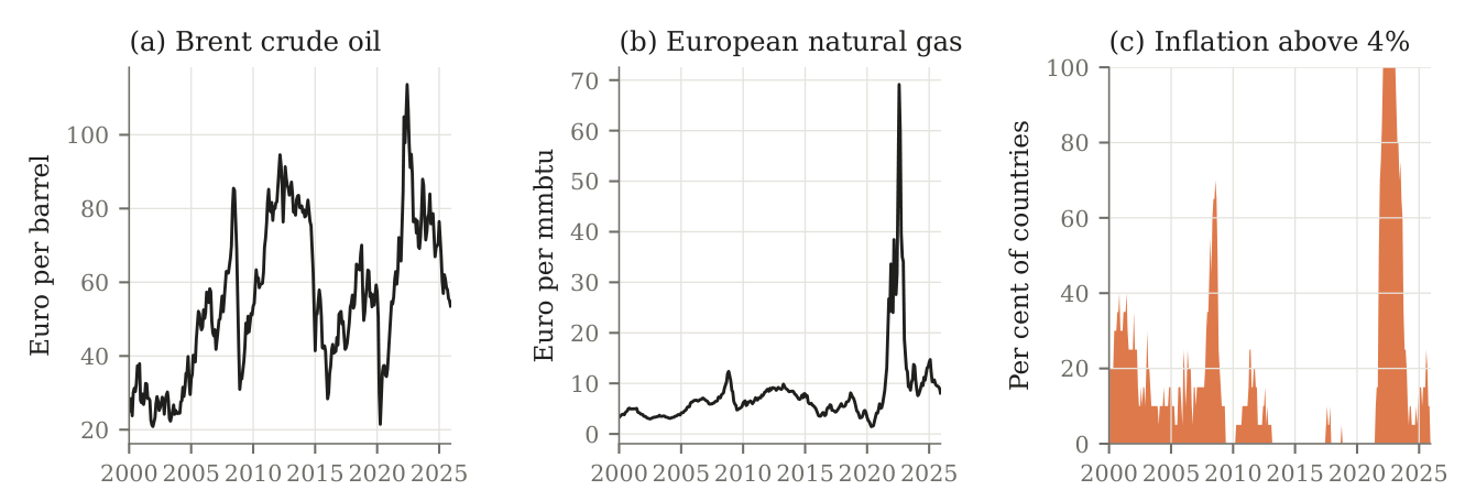
Figure 2.
Linear responses to a 10 per cent energy price innovation. Shaded areas are 90 per cent confidence bands based on Driscoll–Kraay standard errors
Figure 2.
Linear responses to a 10 per cent energy price innovation. Shaded areas are 90 per cent confidence bands based on Driscoll–Kraay standard errors
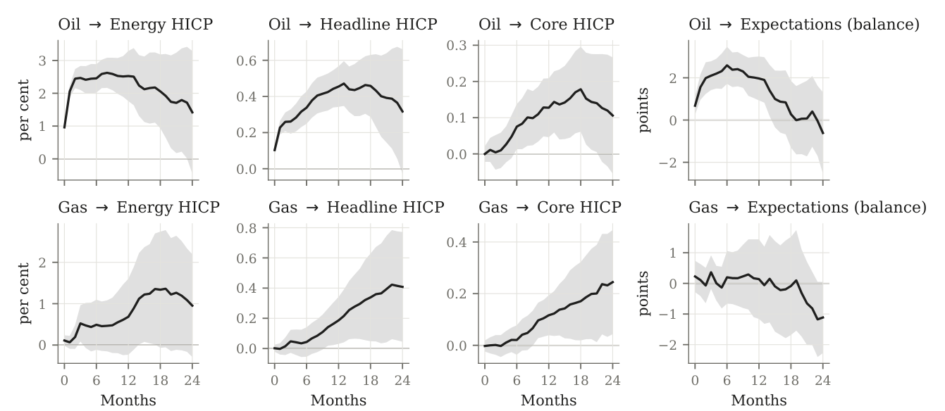
Figure 3.
Responses to a 10 per cent energy price innovation by inflation regime. Shaded areas are 90 per cent confidence bands
Figure 3.
Responses to a 10 per cent energy price innovation by inflation regime. Shaded areas are 90 per cent confidence bands
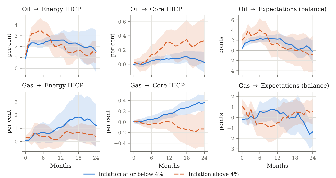
Figure 4.
Leave-one-year-out estimates of the difference between regimes. Each point excludes the impulses of one calendar year; vertical lines are 90 per cent confidence intervals. The dashed line is the full-sample estimate. The highlighted point is the exclusion that moves the estimate most
Figure 4.
Leave-one-year-out estimates of the difference between regimes. Each point excludes the impulses of one calendar year; vertical lines are 90 per cent confidence intervals. The dashed line is the full-sample estimate. The highlighted point is the exclusion that moves the estimate most
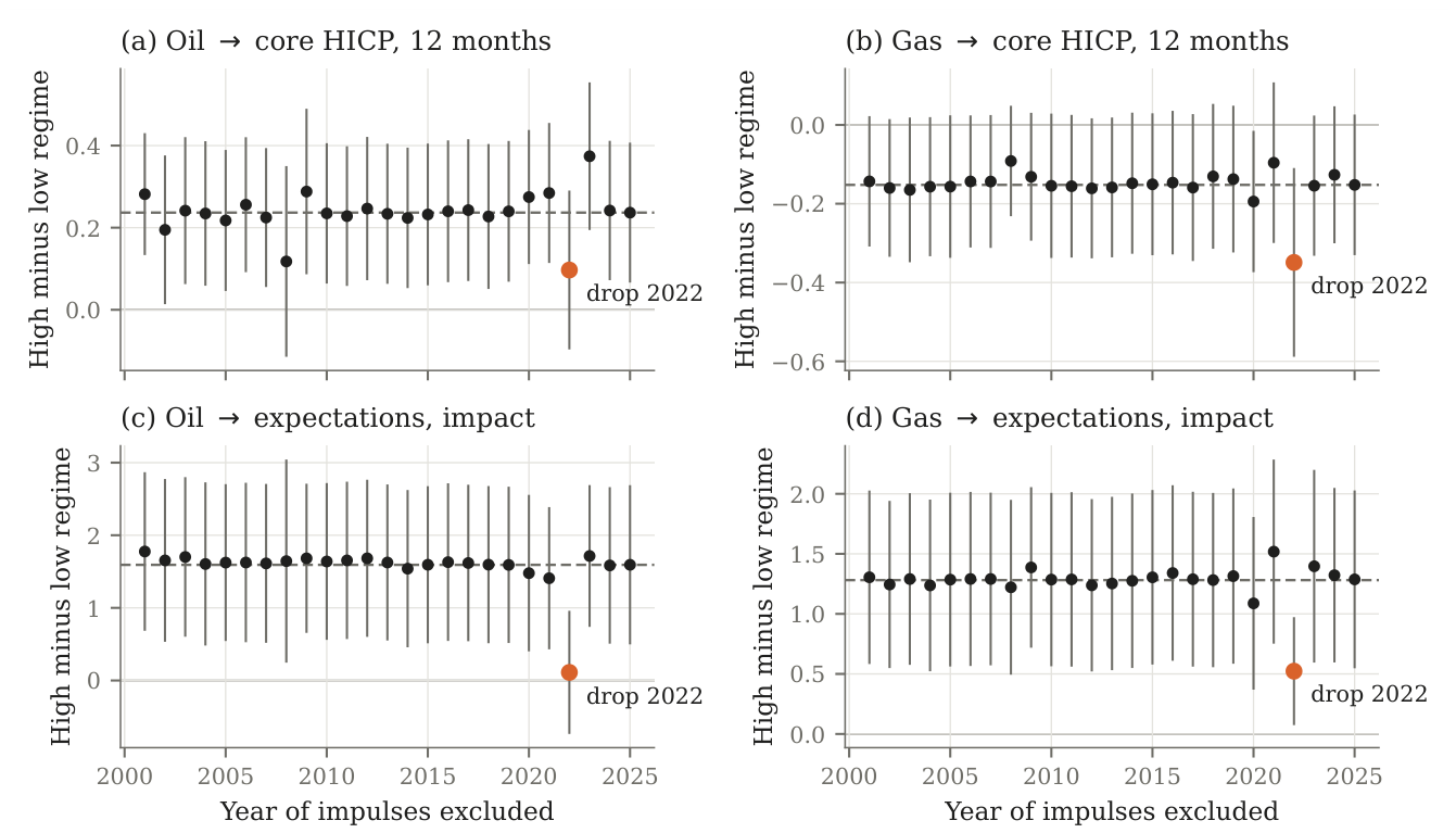
Figure 5.
Difference between high- and low-inflation regimes in the response of core HICP to a 10 per cent innovation. Top row: oil. Bottom row: gas. Shaded areas are 90 per cent confidence bands
Figure 5.
Difference between high- and low-inflation regimes in the response of core HICP to a 10 per cent innovation. Top row: oil. Bottom row: gas. Shaded areas are 90 per cent confidence bands
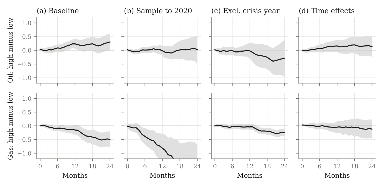
Figure 6.
Fiscal energy support and cumulative price changes, August 2021 to December 2022. Lines are ordinary least squares fits across the twenty countries
Figure 6.
Fiscal energy support and cumulative price changes, August 2021 to December 2022. Lines are ordinary least squares fits across the twenty countries
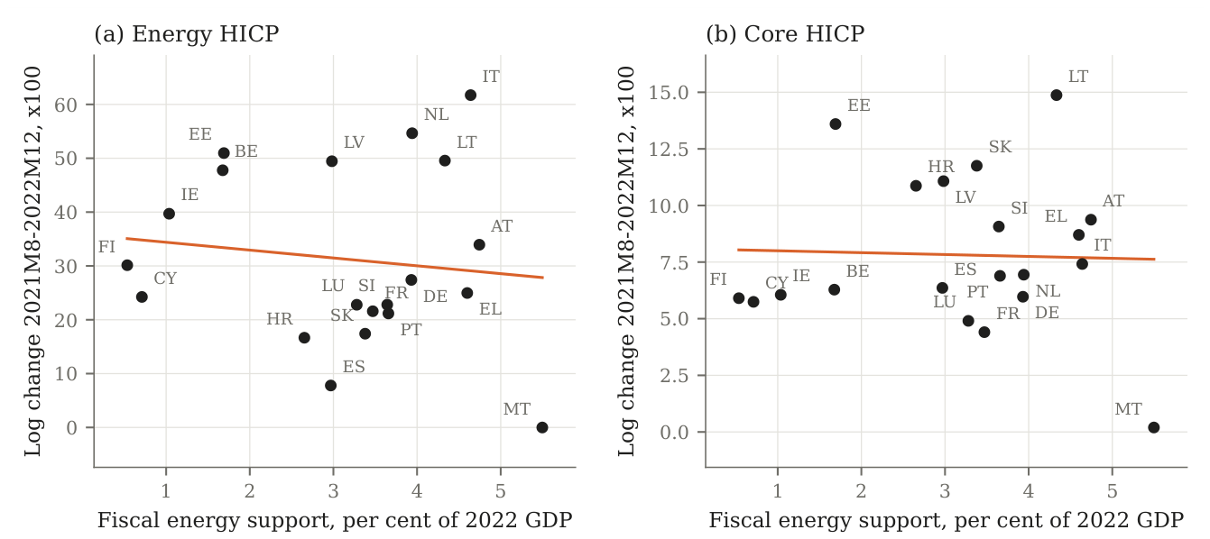
Table 1.
Descriptive statistics, July 2001 to December 2025
| Obs. | Mean | Std. dev. | P10 | Median | P90 | |
| Headline inflation, % | 5880 | 2.51 | 2.70 | −0.01 | 2.08 | 5.19 |
| Core inflation, % | 5865 | 2.00 | 1.90 | 0.30 | 1.67 | 4.27 |
| Energy inflation, % | 5880 | 3.70 | 10.84 | −7.96 | 2.73 | 14.91 |
| Unemployment rate, % | 5880 | 8.61 | 4.34 | 4.40 | 7.50 | 14.40 |
| Price expectations, balance | 5811 | 24.68 | 18.48 | 0.70 | 25.30 | 48.40 |
| Price perceptions, balance | 5811 | 36.38 | 25.80 | 2.30 | 37.10 | 71.50 |
| Oil price innovation, % | 300 | 0.00 | 8.21 | −9.70 | 0.31 | 9.45 |
| Gas price innovation, % | 300 | −0.00 | 9.79 | −11.93 | 0.33 | 9.97 |
Notes: Inflation rates are twelve-month log changes multiplied by 100. Survey variables are seasonally adjusted balances. Innovations are in log points multiplied by 100 and are common to all countries, so they have one observation per month.
Table 2.
Linear responses to a 10 per cent energy price innovation
| Horizon (months) | |||||||
| Impulse | Response | 0 | 3 | 6 | 12 | 18 | 24 |
| Oil | Energy HICP | 0.96 | 2.47 | 2.46 | 2.53 | 2.06 | 1.42 |
| (0.08) | (0.22) | (0.26) | (0.47) | (0.69) | (1.14) | ||
| Oil | Headline HICP | 0.10 | 0.26 | 0.34 | 0.45 | 0.46 | 0.32 |
| (0.02) | (0.04) | (0.05) | (0.07) | (0.10) | (0.21) | ||
| Oil | Core HICP | −0.00 | 0.01 | 0.08 | 0.13 | 0.18 | 0.11 |
| (0.01) | (0.03) | (0.04) | (0.05) | (0.07) | (0.10) | ||
| Oil | Expectations (balance) | 0.68 | 2.10 | 2.59 | 1.97 | 0.28 | −0.61 |
| (0.26) | (0.41) | (0.53) | (0.63) | (0.96) | (1.17) | ||
| Gas | Energy HICP | 0.11 | 0.52 | 0.49 | 0.68 | 1.34 | 0.95 |
| (0.08) | (0.27) | (0.37) | (0.56) | (0.85) | (0.76) | ||
| Gas | Headline HICP | 0.00 | 0.05 | 0.04 | 0.19 | 0.34 | 0.41 |
| (0.01) | (0.05) | (0.06) | (0.09) | (0.18) | (0.22) | ||
| Gas | Core HICP | −0.00 | −0.00 | 0.02 | 0.12 | 0.17 | 0.24 |
| (0.01) | (0.03) | (0.03) | (0.05) | (0.09) | (0.12) | ||
| Gas | Expectations (balance) | 0.23 | 0.37 | 0.20 | 0.14 | −0.08 | −1.11 |
| (0.31) | (0.33) | (0.52) | (0.79) | (0.97) | (0.71) | ||
Notes: Cumulative responses from panel local projections with country-by-calendar-month fixed effects. Price responses are in per cent; the expectations response is in balance points. Driscoll–Kraay standard errors in parentheses.
Table 3.
State-dependent responses to a 10 per cent energy price innovation
| Horizon (months) | ||||||||
| Impulse | Response | Regime | 0 | 3 | 6 | 12 | 18 | 24 |
| Oil | Energy HICP | Low | 0.92 | 2.34 | 2.30 | 2.60 | 2.20 | 1.58 |
| (0.07) | (0.18) | (0.24) | (0.47) | (0.71) | (1.19) | |||
| High | 1.23 | 3.19 | 3.27 | 2.22 | 1.70 | 1.46 | ||
| (0.19) | (0.55) | (0.66) | (0.66) | (0.46) | (0.62) | |||
| p(High = Low) | 0.110 | 0.093 | 0.127 | 0.614 | 0.494 | 0.928 | ||
| Oil | Core HICP | Low | −0.00 | −0.00 | 0.05 | 0.07 | 0.11 | 0.02 |
| (0.01) | (0.02) | (0.03) | (0.04) | (0.05) | (0.09) | |||
| High | 0.03 | 0.02 | 0.14 | 0.31 | 0.34 | 0.33 | ||
| (0.02) | (0.07) | (0.09) | (0.11) | (0.17) | (0.19) | |||
| p(High = Low) | 0.187 | 0.704 | 0.275 | 0.023 | 0.132 | 0.107 | ||
| Oil | Expectations (balance) | Low | 0.41 | 1.99 | 2.32 | 2.22 | 0.52 | −0.29 |
| (0.19) | (0.40) | (0.39) | (0.58) | (0.98) | (1.37) | |||
| High | 2.00 | 2.91 | 4.04 | 1.37 | 0.00 | −0.73 | ||
| (0.64) | (0.89) | (1.40) | (1.57) | (1.92) | (2.14) | |||
| p(High = Low) | 0.016 | 0.279 | 0.166 | 0.550 | 0.755 | 0.854 | ||
| Gas | Energy HICP | Low | 0.06 | 0.58 | 0.72 | 1.07 | 1.79 | 1.22 |
| (0.05) | (0.31) | (0.45) | (0.68) | (1.06) | (0.99) | |||
| High | 0.30 | 0.67 | 0.39 | 0.34 | 0.69 | 0.36 | ||
| (0.11) | (0.44) | (0.57) | (0.43) | (0.39) | (0.45) | |||
| p(High = Low) | 0.031 | 0.859 | 0.640 | 0.286 | 0.298 | 0.422 | ||
| Gas | Core HICP | Low | 0.00 | 0.01 | 0.04 | 0.15 | 0.27 | 0.36 |
| (0.02) | (0.03) | (0.04) | (0.05) | (0.08) | (0.09) | |||
| High | 0.00 | −0.03 | −0.04 | 0.00 | −0.14 | −0.13 | ||
| (0.01) | (0.03) | (0.05) | (0.10) | (0.17) | (0.21) | |||
| p(High = Low) | 0.917 | 0.334 | 0.208 | 0.162 | 0.010 | 0.005 | ||
| Gas | Expectations (balance) | Low | −0.21 | 0.11 | 0.58 | 0.64 | −0.05 | −1.38 |
| (0.15) | (0.39) | (0.61) | (0.73) | (1.02) | (0.81) | |||
| High | 1.07 | 0.75 | −0.56 | −0.52 | 0.57 | 0.57 | ||
| (0.42) | (0.54) | (0.71) | (0.90) | (0.79) | (0.72) | |||
| p(High = Low) | 0.004 | 0.271 | 0.153 | 0.193 | 0.582 | 0.108 | ||
Notes: Estimates of equation (10). High regime: twelve-month headline inflation above 4 per cent in the previous month. Driscoll–Kraay standard errors in parentheses. The last row of each block is the p-value of the test of .
Table 4.
Difference between high- and low-inflation regimes across specifications
| Core HICP, 12 months | Expectations, impact | |||||||
| Oil | Gas | Oil | Gas | |||||
| Specification | Diff. | p | Diff. | p | Diff. | p | Diff. | p |
| Baseline | 0.24 | 0.023 | −0.15 | 0.162 | 1.59 | 0.016 | 1.28 | 0.004 |
| Threshold 3% | 0.18 | 0.022 | −0.08 | 0.321 | 0.91 | 0.047 | 0.82 | 0.058 |
| Threshold 5% | 0.33 | 0.017 | −0.13 | 0.235 | 1.55 | 0.042 | 1.08 | 0.001 |
| Logistic transition | 0.32 | 0.023 | −0.15 | 0.211 | 1.87 | 0.014 | 1.36 | 0.002 |
| Regime: core inflation > 3% | 0.22 | 0.028 | −0.15 | 0.148 | 0.57 | 0.200 | 0.71 | 0.001 |
| Twelve lags | 0.21 | 0.041 | −0.13 | 0.209 | 1.48 | 0.017 | 1.28 | 0.004 |
| Excl. Baltic countries | 0.25 | 0.013 | −0.05 | 0.498 | 2.02 | 0.007 | 1.31 | 0.003 |
| Excl. 2020M3–2020M12 | 0.27 | 0.007 | −0.20 | 0.068 | 1.49 | 0.024 | 1.11 | 0.011 |
| Sample to 2020M12 | −0.02 | 0.888 | −0.82 | 0.009 | 0.09 | 0.886 | 1.67 | 0.069 |
| Excl. 2008M7–2009M6 | −0.02 | 0.904 | −0.04 | 0.548 | 1.75 | 0.024 | 1.37 | 0.001 |
| Time fixed effects | 0.16 | 0.235 | −0.05 | 0.721 | −0.37 | 0.328 | 0.28 | 0.354 |
| Time FE, excl. 2008M7–2009M6 | −0.05 | 0.667 | 0.04 | 0.740 | −0.05 | 0.903 | 0.01 | 0.956 |
| Regime: tight labour market | 0.16 | 0.001 | 0.02 | 0.777 | 0.49 | 0.121 | 0.61 | 0.074 |
Notes: Each entry is , the high-regime response minus the low-regime response to a 10 per cent innovation, with the p-value of the test that it is zero. Core responses are in percentage points; expectations responses are in balance points. Exclusions refer to the month of the impulse. In the last row the regime is an unemployment rate below the country’s sample median.
Table 5.
Fiscal energy support and pass-through
| Horizon (months) | ||||||
| Response | Impulse | Period | 0 | 3 | 6 | 12 |
| Energy HICP | Oil | 2021M9–2023M6 | 0.02 | −0.73 | −0.39 | −0.29 |
| (0.11) | (0.21) | (0.33) | (0.18) | |||
| Other months | −0.05 | −0.32 | −0.23 | −0.15 | ||
| (0.03) | (0.06) | (0.07) | (0.07) | |||
| Gas | 2021M9–2023M6 | 0.02 | 0.09 | 0.09 | 0.07 | |
| (0.04) | (0.12) | (0.08) | (0.06) | |||
| Other months | 0.03 | 0.01 | 0.03 | −0.01 | ||
| (0.03) | (0.07) | (0.10) | (0.16) | |||
| Core HICP | Oil | 2021M9–2023M6 | 0.08 | −0.03 | −0.02 | 0.10 |
| (0.03) | (0.03) | (0.03) | (0.03) | |||
| Other months | 0.00 | −0.02 | −0.01 | 0.01 | ||
| (0.01) | (0.01) | (0.01) | (0.01) | |||
| Gas | 2021M9–2023M6 | −0.04 | 0.02 | −0.01 | −0.04 | |
| (0.01) | (0.02) | (0.01) | (0.01) | |||
| Other months | 0.01 | −0.02 | −0.02 | −0.02 | ||
| (0.01) | (0.01) | (0.01) | (0.02) | |||
| Expectations (balance) | Oil | 2021M9–2023M6 | −0.40 | −0.48 | −0.09 | 0.42 |
| (0.24) | (0.38) | (0.28) | (0.19) | |||
| Other months | −0.28 | −0.30 | −0.09 | 0.11 | ||
| (0.16) | (0.26) | (0.19) | (0.29) | |||
| Gas | 2021M9–2023M6 | −0.07 | 0.05 | −0.08 | −0.11 | |
| (0.16) | (0.14) | (0.17) | (0.05) | |||
| Other months | 0.06 | −0.02 | 0.04 | −0.36 | ||
| (0.09) | (0.24) | (0.16) | (0.26) | |||
Notes: Coefficients on the interaction between a 10 per cent innovation and standardised fiscal energy support (per cent of 2022 GDP), from local projections with country-by-calendar-month and month fixed effects. A negative coefficient means lower pass-through in countries with more support. Driscoll–Kraay standard errors in parentheses.
Table 6.
Summary of predictions and evidence
| Prediction | Full-sample estimate | Episode diagnostics |
| P2: retail energy response equal across regimes | Supported, except for gas in the month of the shock | Oil difference insignificant in all leave-one-year-out samples |
| P1: core response larger at high inflation | Oil: supported (0.31 against 0.07 after one year). Gas: not supported | Oil difference specific to 2008 and 2022; absent in the sample to 2020 |
| P3: impact response of expectations larger at high inflation | Supported for oil and gas | Gas: holds in all leave-one-year-out samples and before 2021. Oil: specific to 2022 |
Disclaimer/Publisher’s Note: The statements, opinions and data contained in all publications are solely those of the individual author(s) and contributor(s) and not of MDPI and/or the editor(s). MDPI and/or the editor(s) disclaim responsibility for any injury to people or property resulting from any ideas, methods, instructions or products referred to in the content. |
© 2026 by the authors. Licensee MDPI, Basel, Switzerland. This article is an open access article distributed under the terms and conditions of the Creative Commons Attribution (CC BY) license (http://creativecommons.org/licenses/by/4.0/).
Copyright: This open access article is published under a Creative Commons CC BY 4.0 license, which permit the free download, distribution, and reuse, provided that the author and preprint are cited in any reuse.