

Submitted:
12 November 2026
Posted:
17 November 2026
You are already at the latest version
Abstract
The Piecewise Polynomial Least Squares Method is a straightforward method to compute accurate approximate analytical solutions for a very wide range of differential problems. The paper presents an extensive study of the method including results regarding the existence and global convergence for the solution and a result regarding the estimation of the error. As an application a fractional-order prey-predator (Lotka-Volterra) model is discussed.
Keywords:
approximate analytical solutions
; differential equations of fractional order
; prey-predator system
; piecewise polynomial least squares method
1. Introduction
The Piecewise Polynomial Least Squares Method (PWPLSM) was recently introduced [1] as a very powerful method of computing analytical approximate solutions for both integer order and fractional order differential problems.
PWPLSM is a part of a larger category of approximation methods including the Adomian Decomposition Method [2], the Homotopy Analysis Method [3], the Variational Iteration Method [4], the Homotopy Perturbation Method [5] or the Optimal Homotopy Asymptotic Method [7]. Although all these approaches have proven their utility for many types of problems, in the case of nonlinear ones they may often exhibit practical limitations such as insufficient accuracy or slow convergence.
In order to overcome such limitations we present PWPLSM, which is based on the Polynomial Least Squares Method (PLSM) [8,9,10], and combines PLSM with a piecewise decomposition of the domain, allowing higher accuracy over long intervals while retaining the analytical, closed-form character of the approximate solution.
In this paper we extend PWPLSM to the fractional-order Lotka–Volterra system
with possibly distinct, are real constants and denoting the Caputo fractional derivative of order [11],
For , system (1) reduces to the classical Lotka–Volterra predator–prey system.
Prey-predator models such this one represent a fundamental application of fractional calculus, studied extensively with various techniques [12,13,14].
In Section 2, by using classical theorems from functional analysis [15,16], we prove the existence and uniqueness of the exact solution for the prey-predator system, as well as global convergence over subintervals for Caputo-type fractional differential equations ([17,18,19]) and in Section 3 we present a full application of PWPLSM for (1).
2. PWPLSM - Method of Solution and Convergence Study
2.1. Description of the Vectorial PWPLSM
Let be divided into equidistant points . On each sub-interval , , we seek an approximate solution pair of (1) of the form
The Caputo derivative of a monomial admits the closed form
which we use, exactly as in the original scalar PWPLSM, to evaluate and termwise. (We return to the subtlety this simplification entails for in Remark 1.)
Residuals and Functional
Definition 1.
An approximate solution pair , , is called aweak -approximate piecewise polynomial solution of (1) if
together with initial and continuity conditions of the type:
On each subinterval we attach to (1) the joint functionals
and determine the coefficients , , that minimize , subject to the continuity constraints above (which fix and ). The polynomials which results are
and define the piecewise PWPLSM solution
2.2. Operator-Theoretic Formulation
The PWPLSM framework via operators between function spaces clarifies the underlying approximation problem. Moreover, this perspective provides an alternative proof for the uniform convergence.
Let denote the Banach space of continuous real-valued functions on endowed with the supremum norm , and let , a Banach space under the norm . For recall the Riemann–Liouville fractional integral operator
a bounded linear Volterra-type integral operator [16,18], compact by the Arzelà–Ascoli theorem (its kernel maps bounded subsets of onto equicontinuous, uniformly bounded families) [16]. For y absolutely continuous on , the Caputo derivative and are related by the fundamental identity
i.e. is a bounded right inverse of modulo the initial value ; see [11,20].
We define the nonlinear operator
with domain consisting of absolutely continuous pairs on . System (1), together with the initial/continuity value, is equivalent to the operator equation
The residual pair of (4) is , i.e. measures the failure of to solve (8); and the least-squares functional (6) is exactly the squared norm of ,
Let be the finite-dimensional affine subspace of polynomial pairs of degree at most m satisfying the prescribed value at . PWPLSM computes
i.e. PWPLSM is a nonlinear least-squares projection method: it seeks the element of lying closest, in the sense, to the zero set of – the operator-theoretic counterpart, for a quadratic operator equation, of Galerkin/Ritz projection methods for linear operator equations. Theorem 5 is then a statement of approximate solvability:
i.e. the images of the nested finite-dimensional subspaces approach the zero element of X, a consequence of the density of polynomials in (Weierstrass) together with the continuity of .
The bilinear term in satisfies an elementary but useful exact identity.
Lemma 1.
For any real-valued functions on , with , ,
identically, with no remainder term, regardless of the size of .
Proof.
. □
Applying Lemma 1 component wise to yields exactly the linear vector operator equation
where , , acts component wise (we take ) and
is a bounded, continuous, matrix-valued coefficient.
Applying to (11) and using (7) with we obtain the equivalent linear Volterra integral equation of the second kind
i.e. , is a bounded linear operator on X, exhibiting the error as a fixed point of the affine map on X.
Lemma 2.
Let and . Then for every and ,
and consequently is quasinilpotent on X: .
Proof.
Since , it results is boundedly invertible on X with Neumann series
converging in operator norm (by Lemma 2, since ). Solving (12) for we have
and, using Lemma 2 with ,
Theorem 1.
With , K, h as above, is bounded and invertible on with , and the error is given explicitly by the Neumann series (14), satisfying . Moreover implies .
Proof.
By Lemma 2, for every , and the scalar series
converges. Since X is a Banach space, absolute convergence of implies that the operator series converges in the operator norm on X, with . A direct telescoping computation shows (the partial sums satisfy in operator norm, since by Lemma 2), so is boundedly invertible with and .
Applying to the exact linear error equation (11) and using the fundamental identity (7) together with we have
i.e. in X.
Multiplying with we obtain
which is (14).
Passing to the norms in (14) and using the bounded operator we obtain,
Also, for any , we have
which results . How ww obtain . □
We establish the existence and uniqueness of the exact solution using the Banach Fixed Point Theorem applied in a weighted Bielecki norm [19]. This approach transforms the nonlinear map below into a contraction, without requiring the length of the sub-interval h to be small for estimating the contraction itself.
Theorem 2.
Let be given (the value of at ), fix , and set , . If is small enough that
then system (1) with initial data , has a unique solution on .
Proof.
By framing (1) via and (7) as in Section 2.2, solves (1) on if and only if is a fixed point of
on the closed ball (functions with , ).
For , , so and point wise, whence and similarly for ; both are smaller then r by (15), so .
For prove the contraction in a Bielecki norm we endow with the equivalent
, and X with .
For any , we have
(bound the integral by ).
For , using Lemma 1-type bounds on we obtain
Selecting a sufficiently large such that ensures that is a contraction on endowed with The latter constitutes a complete metric space, being a closed subset of the Banach space . Consequently, the Banach Fixed Point Theorem guarantees that possesses a unique fixed point in . □
Because PWPLSM transfers the computed value instead of the exact initial condition ) onto the sub-interval establishing control over of the solution with respect to initial data perturbations is essential. This continuous dependence property follows directly from the quasi-nil-potent operator framework introduced in Section 2.2 (Lemma 2), applied here to two apair of exact solutions.
Theorem 3.
Let and be two exact solutions to (corresponding to the same parameters and coefficients ), with initial data and respectively). Assume that both solution pairs are bounded by M on in the sense of Theorem 2. Then, setting and denoting the subinterval length by we have,
where .
Proof.
Defining and , we subtract two exact instances of (1). Applying Lemma 1 in the same manner as in the derivation of (11) - noting that the residual forcing term vanishes since both pairs satisfy the equation exactly yields
where the bounded matrix coefficient is defined as in Section 2.2 (with replaced by, , respectively, both bounded by M). Applying along with (7) leads to the Volterra fixed-point equation where is given by (12) and denotes the constant function equal to ). It follows that . Since by Lemma 2 yields the estimate , which establishes (16). □
2.2.1. A Compactness-Based (Topological) Convergence Result
The estimates established above are entirely quantitative. To complement these, a purely topological convergence result is presented next, utilizing the Arzelà–Ascoli criterion. This approach bypasses the need for explicit error bounds by leveraging the compactness of bounded, equicontinuous subsets of .
Theorem 4.
Suppose the PWPLSM sequence is uniformly bounded and uniformly equicontinuous on (i.e. there exist with as , both independent of m, such that and for all and all m). Then there is a subsequence converging uniformly on to a limit which solves (1) exactly. If, in addition, the exact solution on is unique (as guaranteed by Theorem 2), then and, moreover, thewholesequence converges uniformly to on .
Proof.
By the Arzelà–Ascoli theorem, a uniformly bounded, equicontinuous family in is relatively compact in the uniform topology; hence there is a subsequence converging uniformly on to some . Uniform convergence of to together with uniform boundedness gives uniform convergence of the product (a standard consequence of the algebraic identity together with uniform boundedness of ). How and using the uniform convergence theorem of the polynomial pair, the Caputo derivative operator is bounded and dense defined [18,20], we obtains in . Since is continuous, it results that solves (1) exactly on . Using the uniqueness (Theorem 2), we obtain .
Finally, we obtain that converge uniformly to on . □
Theorem 5.
Let be a sequence of polynomial pairs such that, as ,
uniformly on . Let be the polynomial pair minimizing the functional in (6). Then
Proof.
The existence of the limits for is given by the Weierstrass Approximation Theorem. For to prove non-negativity and monotonicity of
we built, . Moreover, if denotes the finite-dimensional space of polynomial pairs of degree at most m satisfying the fixed boundary value at , then for every m. If, we denote by
we obtain
and results is a non-increasing sequence of non-negative real numbers, hence convergent.
Using the minimality property we obtain
for every .
By hypothesis, how and are uniformly convergent on the compact interval it results that for every there exists such that for all and all , we have
Hence, for , the following inequality holds
and because and is fixed and finite, it follows that
From non-negativity, the inequality (19), and the limit (20), we have
for all .
Using the Contraction Theorem, how for , we obtain,
which is (17). □
3. Application of PWPLSM to the Fractional-Order Prey-Predator Model
3.1. Integer Case
For the classical Lotka-Volterra predator-prey corresponding to , we consider the system (1) with the parameter values , , , , , , , which allows us to compare our approximate solutions with the previous one obtained by using the Differential Transform Method (DTM) in [22].
Using PWPLSM we computed approximations corresponding to several choices of the number of subintervals and of the polynomial degree. For example in the case of 2 subintervals and polynomials of degree 3 we start by choosing the polynomials:
,
where:
,
,
We impose the initial and continuity type conditions:
The polynomials become:
Next we compute the corresponding remainders and functionals (too long to be included here) and by minimization we obtain the values (truncated for convenience):
It follows that the PWPLSM solution for the case of 2 subintervals and polynomials of degree 3 is:
In a similar manner we computed approximations corresponding to other choices of the number of subintervals and of the polynomial degree, the results being illustrated by the following tables and figures. We also include here the PWPLSM solution for the case of 4 subintervals and polynomials of degree 4 as relatively simple but accurate approximation:
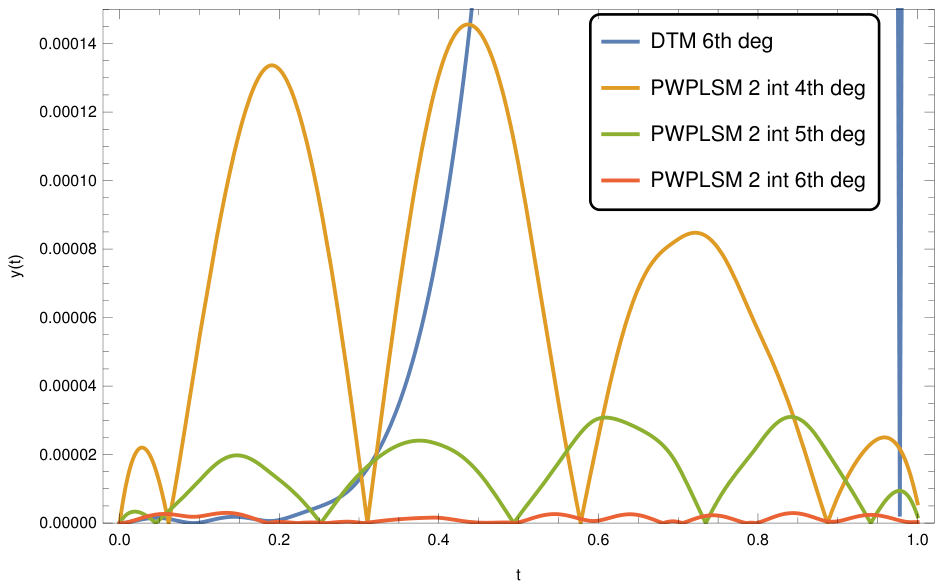
We compared our results with the results in [22] obtained by using the Differential Transform Method (DTM). Since for the given problem no exact analytical solution is known, we will compute the error corresponding to each approximation as the difference (in absolute value) between the approximation itself and the result obtained by applying a Runge-Kutta type method. The following Tables and Figures (1 to 4) present a comparative analysis of these errors for several choices of the number of subintervals and several choices of the polynomial degrees.
Not only do this results emphasize the accuracy of our approximations but at the same time they illustrate the convergence of the method, since by increasing both the number of subintervals and the degrees of the polynomials we obtain smaller errors.

Table 1.
Comparison of errors for x(t): 6th degree DTM solution vs. 4th degree PWPLSM with different number of subintervals
Table 1.
Comparison of errors for x(t): 6th degree DTM solution vs. 4th degree PWPLSM with different number of subintervals
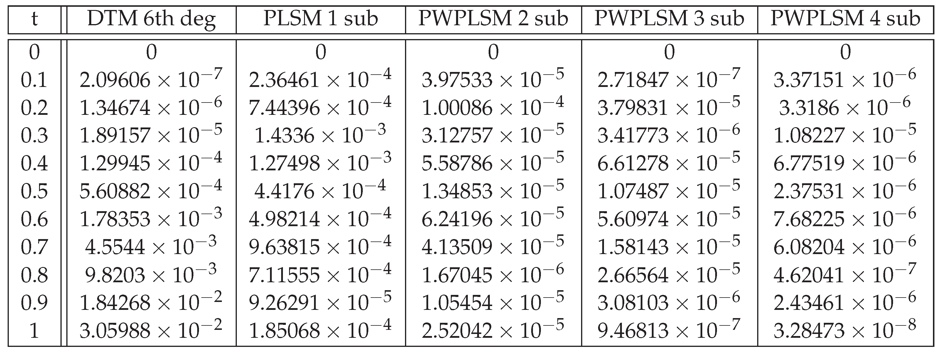
Table 2.
Comparison of errors for y(t): 6th degree DTM solution vs. 4th degree PWPLSM with different number of subintervals
Table 2.
Comparison of errors for y(t): 6th degree DTM solution vs. 4th degree PWPLSM with different number of subintervals
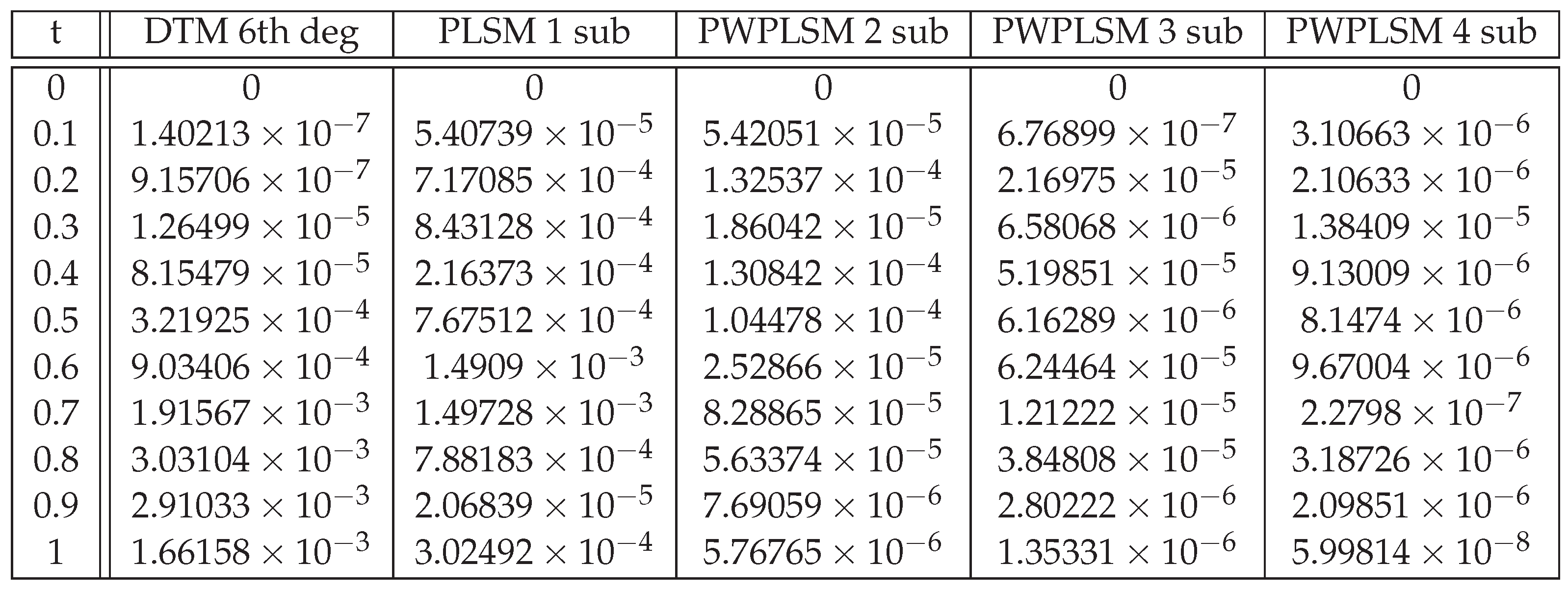
Figure 1.
Comparison of errors for x(t): 6th degree DTM solution vs. 4th degree PWPLSM with different number of subintervals
Figure 1.
Comparison of errors for x(t): 6th degree DTM solution vs. 4th degree PWPLSM with different number of subintervals
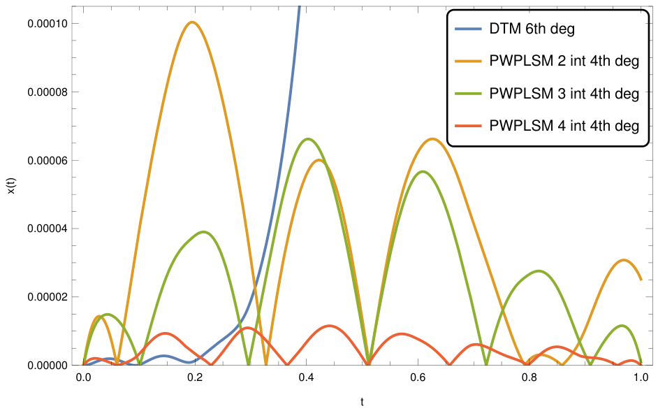
Figure 2.
Comparison of errors for y(t): 6th degree DTM solution vs. 4th degree PWPLSM with different number of subintervals
Figure 2.
Comparison of errors for y(t): 6th degree DTM solution vs. 4th degree PWPLSM with different number of subintervals
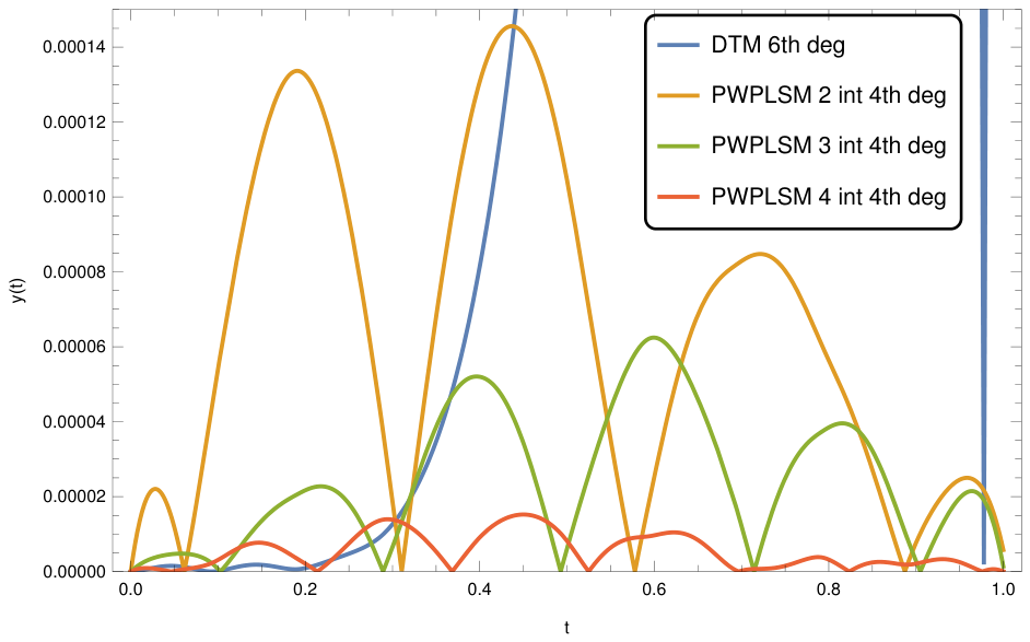
Table 3.
Comparison of errors for x(t): 6th degree DTM solution vs. PWPLSM on 2 subintervals with different polynomial degrees
Table 3.
Comparison of errors for x(t): 6th degree DTM solution vs. PWPLSM on 2 subintervals with different polynomial degrees
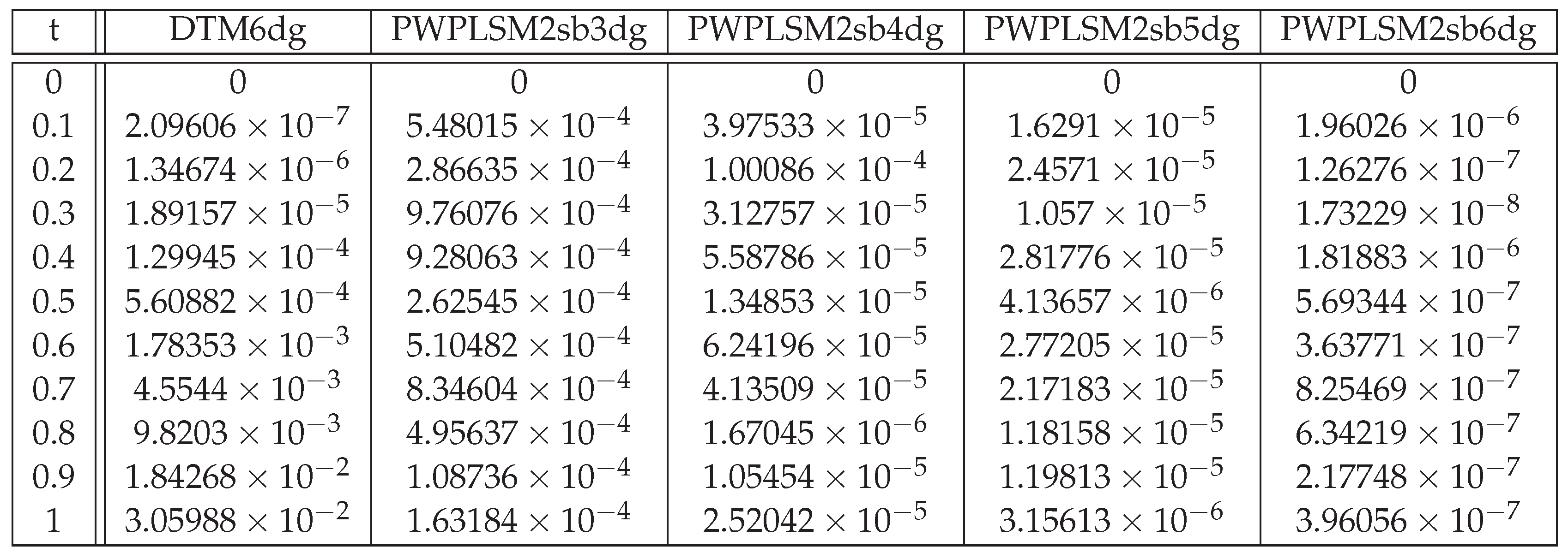
Table 4.
Comparison of errors for y(t): 6th degree DTM solution vs. PWPLSM on 2 subintervals with different polynomial degrees
Table 4.
Comparison of errors for y(t): 6th degree DTM solution vs. PWPLSM on 2 subintervals with different polynomial degrees
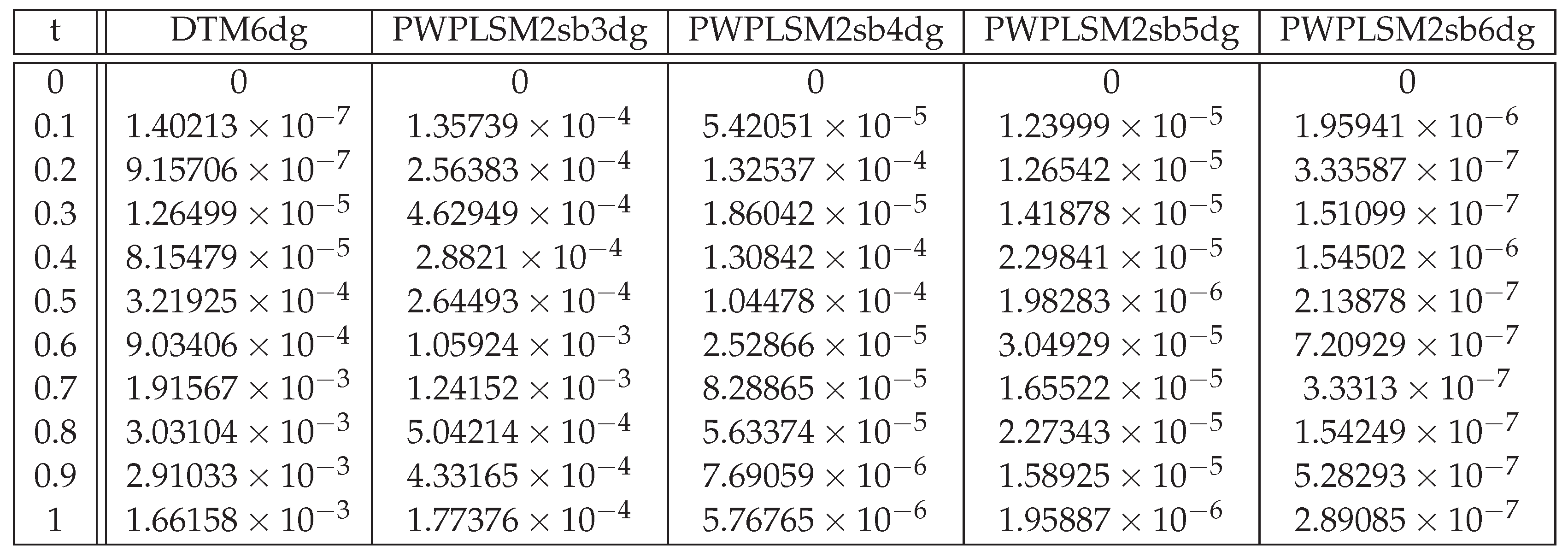
Figure 3.
Comparison of errors for x(t): 6th degree DTM solution vs. PWPLSM on 2 subintervals with different polynomial degrees
Figure 3.
Comparison of errors for x(t): 6th degree DTM solution vs. PWPLSM on 2 subintervals with different polynomial degrees
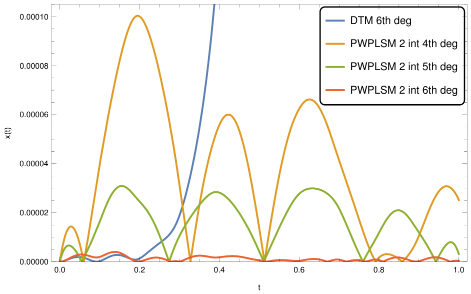
Figure 4.
Comparison of errors for y(t): 6th degree DTM solution vs. PWPLSM on 2 subintervals with different polynomial degrees
Figure 4.
Comparison of errors for y(t): 6th degree DTM solution vs. PWPLSM on 2 subintervals with different polynomial degrees
3.2. Fractional Case
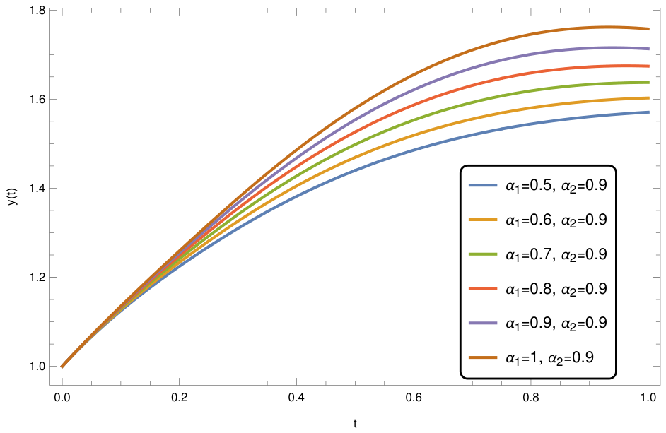
PWPLSM can be successfully applied also in the fractional case of the predator-prey model. For example, by using the Caputo derivative for and choosing 4 intervals and polynomials of degree 4 we computed the approximate solution:
4. Conclusions
In this paper we extended the recently introduced Piecewise Polynomial Least Squares Method to a nonlinearly coupled fractional-order predator-prey system.
While we previously employed PWPLSM in the case of several simpler problems, the present study also introduces an extensive novel qualitative study of the method including several important results concerning the existence and global convergence of the solution and the error estimation.
The presented application, which also includes a comparison with results of a previous study, illustrate the high accuracy of the method.
Future work may include: (i) a memory-corrected variant of the piecewise Caputo derivative formula, addressing the simplification of Remark 1; (ii) an analytic (rather than empirical) criterion for choosing the regularization strength ; and (iii) application of PWPLSM to other coupled fractional systems arising in epidemiology (SIR-type models) and viscoelasticity (Bagley–Torvik-type systems).
Author Contributions
Conceptualization, Mădălina Sofia Paşca, Adina Juratoni, Olivia Bundău, Bogdan Căruntu; methodology, Mădălina Sofia Paşca; software, Bogdan Căruntu; validation, Olivia Bundău; formal analysis, Adina Juratoni; writing—original draft preparation, Mădălina Sofia Paşca, Adina Juratoni, Olivia Bundău, Bogdan Căruntu; writing—review and editing, Mădălina Sofia Paşca, Adina Juratoni, Olivia Bundău, Bogdan Căruntu. All authors have read and agreed to the published version of the manuscript.
Funding
This research received no external funding.
Institutional Review Board Statement
Not applicable.
Informed Consent Statement
Not applicable.
Data Availability Statement
Data is contained within the article.
Conflicts of Interest
The authors declare no conflicts of interest.
References
- M. S. Paşca, Piecewise Polynomial Least Squares Method for Differential Equations of Fractional Order, Annals of West University of Timisoara, Mathematics and Computer Science 59 (2023), 69–78. [CrossRef]
- G. Adomian, A Review of the Decomposition Method in Applied Mathematics, Journal of Mathematical Analysis and Applications, 135 (1988), 501–544. [CrossRef]
- S.J. Liao, Homotopy analysis method: A new analytical technique for nonlinear problems, Communications in Nonlinear Science and Numerical Simulation, 2 (1997), 95–100. [CrossRef]
- J.H. He, Variational iteration method - a kind of non-linear analytical technique: some examples, International Journal of Non-Linear Mechanics, 34 (1999), 699–708. [CrossRef]
- J.H. He, Homotopy perturbation technique, Computer Methods in Applied Mechanics and Engineering, 178 (1999), 257–262. [CrossRef]
- He, J.H. Homotopy perturbation technique, Computer Methods in Applied Mechanics and Engineering. Int. J. Nonlinear Mech. 1999, 178, 257–262, . [CrossRef]
- V. Marinca, N. Herisanu, I. Nemes, Optimal Homotopy Asymptotic Method with Application to Thin Film Flow, Open Physics, 6 (2008), 648–653. [CrossRef]
- C. Bota, B. Căruntu, Approximate Analytical Solutions of the Fractional-Order Brusselator System Using the Polynomial Least Squares Method, Advances in Mathematical Physics 2015, Article ID 450235, 5 pages.
- C. Bota, B. Căruntu, Analytical approximate solutions for quadratic Riccati differential equation of fractional order using the Polynomial Least Squares Method, Chaos, Solitons and Fractals 102 (2017), 339–345. [CrossRef]
- B. Căruntu, C. Bota, M. Lăpădat, M. S. Paşca, Polynomial Least Squares Method for Fractional Lane–Emden Equations, Symmetry 11(4) (2019), 479. [CrossRef]
- I. Podlubny, Fractional Differential Equations, Mathematics in Science and Engineering, vol. 198, Academic Press, San Diego, 1999.
- A. El-Mesady, A. M. Elsonbaty, W. Adel, Insight into Caputo Fractional-Order Extension of the Lotka–Volterra Model with Emphasis on Immigration Effect, Journal of Mathematics 2023, Article ID 8795660. [CrossRef]
- P. A. Patel et al., Analyzing the nonlinear fractional Lotka–Volterra model for prey–predator system via a novel wavelets approach, Franklin Open (2025), ScienceDirect, article in press. [CrossRef]
- A. S. V. Ravi Kanth, S. Devi, A practical numerical approach to solve a fractional Lotka–Volterra population model with non-singular and singular kernels, Chaos, Solitons and Fractals 145 (2021), 110792. [CrossRef]
- A. Bielecki, Une remarque sur la méthode de Banach–Cacciopoli–Tikhonov dans la théorie des équations différentielles ordinaires, Bulletin de l’Académie Polonaise des Sciences, Classe III 4 (1956), 261–264.
- C. Corduneanu, Integral Equations and Applications, Cambridge University Press, Cambridge/New York, 1991.
- K. Diethelm, N. J. Ford, Analysis of fractional differential equations, Journal of Mathematical Analysis and Applications 265(2) (2002), 229–248. [CrossRef]
- A. A. Kilbas, H. M. Srivastava, J. J. Trujillo, Theory and Applications of Fractional Differential Equations, North-Holland Mathematics Studies, vol. 204, Elsevier, Amsterdam, 2006.
- V. Lakshmikantham, A. S. Vatsala, Basic theory of fractional differential equations, Nonlinear Analysis: Theory, Methods & Applications 69(8) (2008), 2677–2682. [CrossRef]
- K. Diethelm, The Analysis of Fractional Differential Equations, Lecture Notes in Mathematics, Springer, Berlin, 2010.
- E. Kreyszig, Introductory Functional Analysis with Applications, Wiley, New York, 1978.
- A.A. Adeniji, H.A. Noufe, A.C. Mkolesia, M.Y. Shatalov, An Approximate Solution to Predator-prey Models Using The Differential Transform Method and Multi-step Differential Transform Method, in Comparison with Results of The Classical Runge-kutta Method, Mathematics and Statistics, 9 (2021), 799–805. [CrossRef]
Figure 5.
x(t) PWPLSM for and several values of
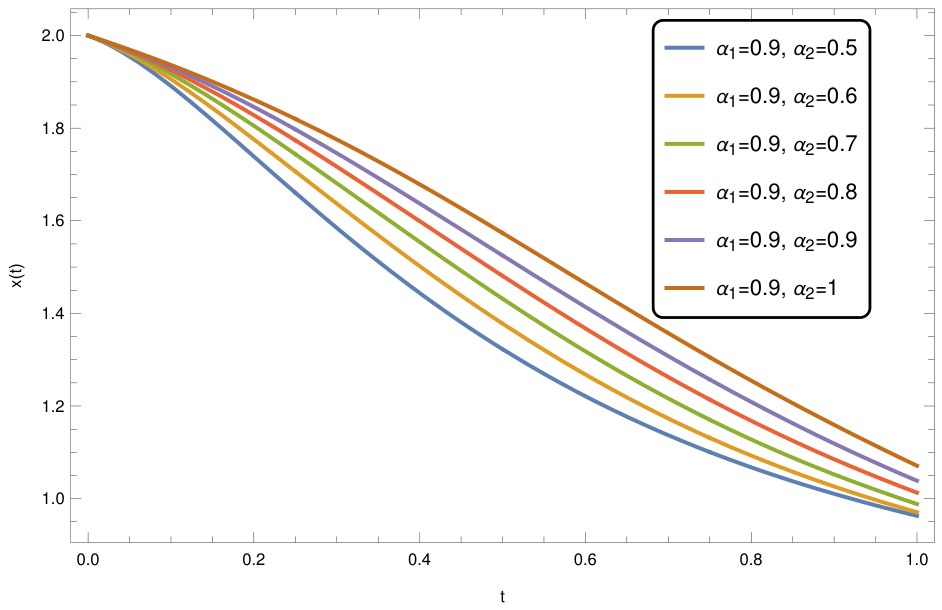
Figure 6.
y(t) PWPLSM for and several values of
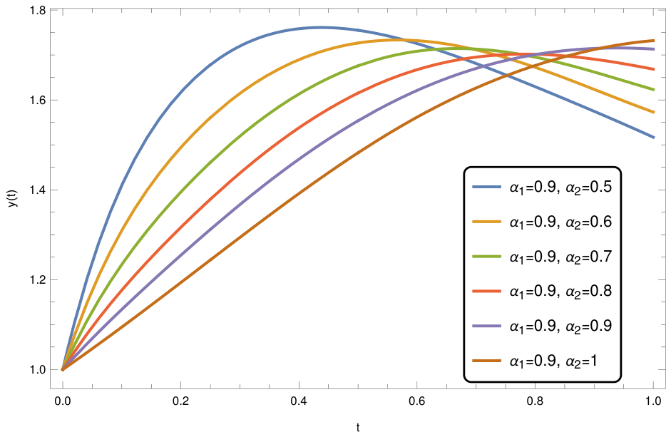
Figure 7.
x(t) PWPLSM for several values of
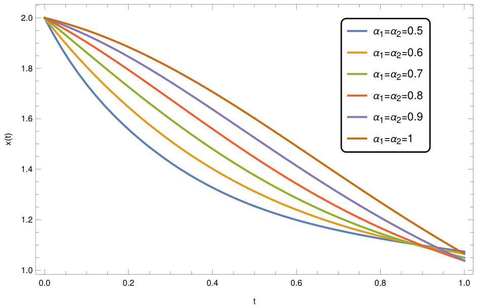
Figure 8.
y(t) PWPLSM for several values of
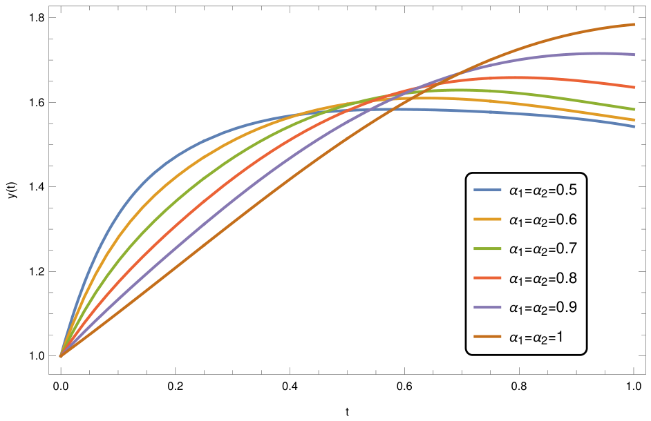
Figure 9.
x(t) PWPLSM for and several values of
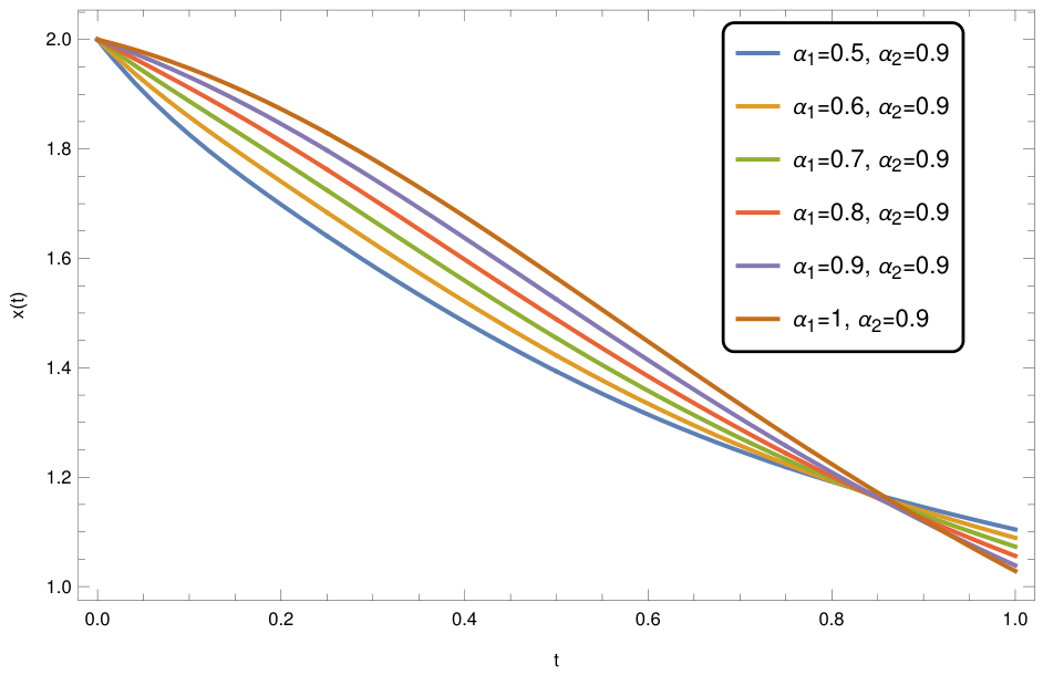
Figure 10.
y(t) PWPLSM for and several values of
Disclaimer/Publisher’s Note: The statements, opinions and data contained in all publications are solely those of the individual author(s) and contributor(s) and not of MDPI and/or the editor(s). MDPI and/or the editor(s) disclaim responsibility for any injury to people or property resulting from any ideas, methods, instructions or products referred to in the content. |
© 2026 by the authors. Licensee MDPI, Basel, Switzerland. This article is an open access article distributed under the terms and conditions of the Creative Commons Attribution (CC BY) license (http://creativecommons.org/licenses/by/4.0/).
Copyright: This open access article is published under a Creative Commons CC BY 4.0 license, which permit the free download, distribution, and reuse, provided that the author and preprint are cited in any reuse.