
Submitted:
13 November 2026
Posted:
16 November 2026
You are already at the latest version
Abstract
Arsenic contamination of the Kok River in northern Thailand is currently monitored by manual sampling at fixed points, and laboratory results take three to four weeks, while the source often remains unknown. We present NEXUSFlow, a monitoring system in which a fleet of five autonomous surface vehicles surveys a river reach along automatically planned zigzag routes, a plume-mapping model (PatternTrack AI) estimates the contaminant field and traces its source, and an AI agent (NATEE) drafts a response plan that is released only after approval by a pollution control officer and a village leader. To test the central design choice—mobile zigzag sampling instead of fixed stations—we ran a Monte Carlo simulation of 2,000 bank-side discharges in a 12 km reach using a two-dimensional transverse-mixing model with reflecting banks. The median full-mixing length was 46 km, so plumes remained attached to one bank throughout the reach. In the 1,776 scenarios in which some location exceeded 0.01 mg/L, seven fixed stations on one bank detected the plume in 38% of cases, stations on both banks in 75%, mid-channel stations in 2% and a centreline boat in 4%, whereas a 40-sample zigzag survey detected 83%. A short follow-up along the affected bank reduced the median source-location error to 15 m, compared with about 830 m for fixed stations. The ranking was unchanged for strongly meandering reaches. A prototype run on simulated data took 81 min from the first report to a village alert. The results support combining mobile zigzag surveys with fixed stations and must be confirmed by field tests.
Keywords:
arsenic
; autonomous surface vehicle
; river monitoring
; source localization
; transverse mixing
; zigzag survey
1. Introduction
The Kok River flows through Chiang Mai and Chiang Rai provinces in northern Thailand before joining the Mekong River, and it has suffered from recurring arsenic contamination. The Pollution Control Department (PCD) monitors water and sediment at 15 stations along the Kok River (KK01–KK15), together with tributaries, the Sai River and the Mekong River (Thai PBS, 2025). In the 19th monitoring round, samples were collected on 19–22 May 2026 and results were released on 15 June 2026, reporting arsenic above the 0.01 mg/L standard at four points on the Kok River (Thai PBS, 2026). The delay between sampling and public results is therefore three to four weeks, and the reported source remained uncertain.
Two physical facts make this problem difficult for fixed monitoring. First, most discharges enter a river at the bank, and a contaminant mixes over the depth quickly but across the channel slowly; a bank discharge may need tens to hundreds of kilometres to become fully mixed (Fischer et al., 1979; Pilechi et al., 2015). Second, the bank acts as a reflecting boundary, so the plume remains a narrow band along one bank (Bielski, 2021). A fixed sampler on the other bank, or in mid-channel, can read safe values while the outfall bank is contaminated. Fixed samplers also cannot capture spatial variability in large water bodies (Mamani et al., 2025), whereas sensor-equipped surface vehicles can map water quality at much higher spatial resolution than manual sampling (Griffiths et al., 2022) and have revealed localised peaks downstream of drain outlets (Griffiths et al., 2020).
Robotics offers two relevant tools. Coverage path planning provides routes that let a sensor cover an area efficiently (Galceran & Carreras, 2013); for rivers, the Z-Cover method lets a vessel zigzag downstream and cover the full width in one pass (Karapetyan et al., 2019). Plume source localization uses autonomous vehicles as mobile sensors to build a probability map of the source position (Pang & Farrell, 2006), typically in search, tracking and source-declaration phases (Li et al., 2026).
This paper makes three contributions: (i) we describe the NEXUSFlow system, which combines a multi-boat zigzag survey, plume mapping and an AI planning agent with human approval; (ii) we quantify, by Monte Carlo simulation, how well zigzag surveys detect and locate bank-side sources compared with fixed stations and centreline surveys; and (iii) we report a prototype run of the full workflow on simulated data.
2. Materials and Methods
2.1. System Overview
NEXUSFlow has four components (Figure 1). (1) Fleet. Five autonomous surface vehicles carry arsenic sensors and survey an assigned 12 km reach; the dashboard shows each boat’s task, battery level and latest reading. (2) Route planning. When an officer selects a river section, zigzag routes that alternate between the two banks and mid-channel are planned automatically. After an exceedance, a boat follows the affected bank upstream until readings fall below the limit and then circles the suspected outfall. (3) PatternTrack AI. Readings are combined into a concentration map of the reach, the plume is traced to a suspected source, and its movement over the next 60 min is forecast. (4) NATEE agent. An AI agent ranks high-risk zones and drafts a response plan (field inspection, laboratory samples and community alerts). Because people tend to reject algorithms after seeing errors but accept them when they can modify the output (Dietvorst et al., 2018), the plan is released only after a pollution control officer approves or edits it, and alerts reach residents by LINE and SMS only after a village leader confirms them. Boat readings are used for screening and targeting; confirmation still relies on laboratory analysis. The workflow was developed in consultation with five specialists from the Environmental and Pollution Control Office 1, Chiang Mai.
2.2. Dispersion Model
To evaluate the sampling strategy, we simulated a straight 12 km reach, equal to the reach shown on the dashboard. The steady-state, depth-averaged concentration from a continuous bank-side source was obtained from the two-dimensional advection–diffusion equation (Fischer et al., 1979), with the method of images representing the impermeable banks:
where s = x − xs + x0 for x > xs (upstream of the outfall C = Cb); Cb is the background concentration; M the mass loading rate; d depth; U velocity; W width; y0 the outfall bank; xs the outfall position; x0 = 50 m a virtual origin that avoids the singularity at the outfall; f the friction factor; and α the transverse mixing constant, about 0.15 for straight uniform channels, 0.4 for natural channels and 0.6 (±50%) for meandering channels (Fischer et al., 1979). The full-mixing length was taken as L≈0.4UW2/εt. We verified that the cross-sectional mean excess concentration equals M/(UdW) at every distance, confirming mass conservation.
2.3. Scenarios
We drew 2,000 parameter sets (Table 1). The ranges are assumptions for a medium river resembling the Kok River near Chiang Rai, not field measurements. Every reading received random error of 10% of the value plus 0.0005 mg/L to represent sensor error. The simulation was written in Python (NumPy) with random seed 20261112.
2.4. Sampling Designs and Metrics
All samples were at least 5 m from a bank. We compared: (1) 7 fixed stations every 2 km on one bank; (2) 14 fixed stations every 2 km on both banks; (3) 7 fixed mid-channel stations, comparable to bridge sampling; (4) a boat on the centreline taking 40 samples every 300 m; (5) a zigzag boat taking 40 samples every 300 m, cycling bank 1, mid-channel, bank 2, mid-channel (the NEXUSFlow design), plus the same pattern with 20 samples (600 m) and 80 samples (150 m); and (6) the zigzag boat with bank follow-up, in which, after an exceedance, the boat moves upstream along the affected bank sampling every 50 m (at most 40 samples) until readings fall below the limit.
The detection rate is the share of scenarios in which at least one reading exceeds 0.01 mg/L, computed over scenarios in which the true field exceeds the limit somewhere in the sampled area. The source-location error is the along-stream distance between the most upstream exceedance and the true outfall (for follow-up, the last exceedance minus 25 m), computed over detected scenarios and reported as the median and 90th percentile (P90).
2.5. Prototype Run
The complete workflow (report, boat launch, survey, source trace, plan approval and alert) was run once on the prototype dashboard with a simulated arsenic event in a 12 km section of the Kok River. Times in the run are produced by the prototype and simulated data, not by field operation.
2.6. Use of Generative AI
The authors used Claude (Anthropic) to assist with literature search, simulation code and manuscript preparation. The authors reviewed all content and take full responsibility for the article.
3. Results
3.1. Plume Behaviour
Of the 2,000 scenarios, 1,776 (88.8%) contained an exceedance in the sampled area. The median full-mixing length was 46 km (10th percentile 17 km), longer than the 12 km reach in almost every case. In 98.6% of polluted scenarios, the fully mixed concentration would be below 0.01 mg/L; the hazardous zone is therefore only a band along the outfall bank, and samples taken in mid-channel or on the opposite bank read as safe (Figure 2).
3.2. Detection and Source Location
Table 2 and Figure 3 summarise the results. One-bank fixed stations detected 74.2% of plumes when the outfall was on their bank but only 0.6% when it was on the opposite bank (38.2% overall). Stations on both banks raised detection to 75.1%, but the location error remained about 830 m because it is limited by station spacing. Mid-channel sampling, by stations or by boat, detected only 2–4%. The 40-sample zigzag boat detected 82.6%, nearly independent of the outfall bank (82.0% and 83.2%). Sample spacing mattered: 20, 40 and 80 samples detected 72.2%, 82.6% and 90.5%, respectively. With bank follow-up, using about 12 additional samples on average, the median location error fell to 15 m (P90 = 96 m). In every detected scenario, the first exceedance occurred on the outfall bank, so the boat always knew which bank to follow.
3.3. Sensitivity Analysis
With α = 0.6–2.5, representing strongly meandering reaches that mix much faster, the median full-mixing length fell to 18 km (10th percentile 7 km). The ranking of designs was unchanged: the 40-sample zigzag detected 69.3%, both-bank stations 59.6%, one-bank stations 29.3% and the centreline boat 7.7%, and bank follow-up still achieved a median error of 14 m.
3.4. Prototype Run
In the prototype run on simulated data (Figure 1), the officer launched five boats at 05:42 after a report of discoloured water. The boats collected 40 readings in about 30 min, followed the affected bank upstream and circled a bank pipe at km 7.1, which PatternTrack AI marked as the suspected source with 81% confidence. At 06:41, NATEE proposed sampling Zone 6 (peak 0.038 mg/L), inspecting the pipe with three laboratory samples, and warning Zone 7 first because the forecast showed the plume exceeding the limit there within 60 min. A fixed sensor in Zone 7 read 0.008 mg/L at that time. After approval by the officer and confirmation by the village leader, 214 households received LINE and SMS alerts at 07:03, 81 min after the first report.
4. Discussion
A bank-side discharge forms a long, narrow band attached to one bank. A fixed sampling point sees this band only if it is on the same bank and downstream of the outfall. The zigzag survey alternately samples both banks and mid-channel, visiting each bank every 1.2 km, and therefore detects plumes almost equally well on either bank. The more important advantage is mobility: once an exceedance is found, the boat can trace the affected bank upstream, reducing the location error from hundreds of metres to tens of metres. Fixed stations cannot do this regardless of their number, because their spatial resolution is limited by station spacing. This sequence follows the search, tracking and declaration structure of autonomous source localization (Li et al., 2026) and extends the full-width zigzag coverage idea of Z-Cover (Karapetyan et al., 2019) to contaminant monitoring.
These results do not imply that fixed sensors are unnecessary. Fixed sensors provide high temporal but coarse spatial resolution, whereas sensor-equipped boats provide high spatial resolution (Griffiths, 2021). Fixed stations are suited to trend monitoring and to alerts when contamination reaches critical points such as water-supply intakes; boats are suited to finding where contamination is and where it comes from. The prototype run also illustrates the time gap: a fixed sensor downstream read 0.008 mg/L while the forecast indicated an exceedance within the hour.
This study has limitations. The model assumes a straight channel at steady state and omits bends, secondary currents, tributaries, intermittent discharges and sediment resuspension, which is important for arsenic in the Kok River; the parameter ranges are assumptions. Sensor response time, current forces on navigation, obstacles and battery capacity were not modelled. The follow-up in the simulation is a simple rule, and the accuracy of PatternTrack AI and NATEE was not evaluated here. The prototype run used simulated data and a single event. Future work should compare boat readings with laboratory analyses at the same points on the Kok River, evaluate zigzag spacings of 150–300 m within time and battery limits, test adaptive spacing that samples sparsely where readings are low and densely as they rise, and evaluate the plume model against field data.
5. Conclusions
River-mixing theory and a 2,000-scenario simulation show that a bank-side discharge stays on one bank over long distances, so fixed-point and centreline sampling easily miss it. A 40-sample zigzag boat survey detected 83% of plumes, and a short follow-up along the affected bank located the source to within about 15 m, compared with about 830 m for fixed stations. NEXUSFlow combines this survey strategy with plume mapping and an AI planning agent under human approval. These results support combining mobile zigzag surveys with fixed stations; field tests on the Kok River are the next step.
Data Availability Statement
Simulation code and output data are available from the corresponding author on request. Results are reproducible with the random seed given in Section 2.3.
Acknowledgments
The authors thank the specialists of the Environmental and Pollution Control Office 1, Chiang Mai, for consultation on the officer workflow.
Conflicts of Interest
The authors declare no conflicts of interest.
References
- Bielski, A. (2021). Mixing effects in the river downstream from pollution discharge point. Technical Transactions, e2021004. [CrossRef]
- Dietvorst, B. J., Simmons, J. P., & Massey, C. (2018). Overcoming algorithm aversion: People will use imperfect algorithms if they can (even slightly) modify them. Management Science, 64(3), 1155–1170. [CrossRef]
- Fischer, H. B., List, E. J., Koh, R. C. Y., Imberger, J., & Brooks, N. H. (1979). Mixing in inland and coastal waters. Academic Press.
- Galceran, E., & Carreras, M. (2013). A survey on coverage path planning for robotics. Robotics and Autonomous Systems, 61(12), 1258–1276.
- Griffiths, N. A. (2021). Spatially resolved measurements of water quality indicators within a bioenergy landscape [Conference presentation]. U.S. Department of Energy, Bioenergy Technologies Office Project Peer Review. https://www.energy.gov/sites/default/files/2021-04/beto-17-peer-review-2021-analysis-griffiths.pdf.
- Griffiths, N. A., et al. (2020). A novel unmanned surface vehicle-sensor platform for mapping water quality in streams and rivers in the agricultural Midwest [Conference abstract]. AGU Fall Meeting 2020. https://ui.adsabs.harvard.edu/abs/2020AGUFMH120…08G.
- Griffiths, N. A., Levi, P. S., Riggs, J. S., DeRolph, C. R., Fortner, A. M., & Richards, J. K. (2022). Sensor-equipped unmanned surface vehicle for high-resolution mapping of water quality in low- to mid-order streams. ACS ES&T Water, 2, 425–435. [CrossRef]
- Karapetyan, N., Braude, A., Moulton, J., Burstein, J. A., White, S., O’Kane, J. M., & Rekleitis, I. (2019). Riverine coverage with an autonomous surface vehicle over known environments. arXiv:1908.02827.
- Li, Z., Hollenbeck, D., Wu, R., Sherman, M., Shao, S., & Sun, X. (2026). Multi-agent reinforcement learning for UAV-based chemical plume source localization. arXiv:2603.11582.
- Mamani, M., Fernandez, M., Luna, G., Limachi, S., Apaza, L., Montes-Dávalos, C., Herrera, M., & Salcedo, E. (2025). High-resolution water sampling via a solar-powered autonomous surface vehicle. arXiv:2512.09798.
- Pang, S., & Farrell, J. A. (2006). Chemical plume source localization. IEEE Transactions on Systems, Man, and Cybernetics, Part B (Cybernetics), 36(5), 1068–1080.
- Pilechi, A., Rennie, C. D., Mohammadian, A., & Zhu, D. Z. (2015). In situ spatially distributed field measurements of transverse dispersion of a wastewater effluent in an extended natural meandering river. Journal of Hydraulic Research, 53(1), 20–35. https://doi.org/10.1080/00221686.2014.950611. [CrossRef]
- Thai PBS. (2025). Fourth test round: Arsenic exceeds the standard at 15 points on the Kok River and 3 points on the Sai River [in Thai]. https://www.thaipbs.or.th/news/content/353065.
- Thai PBS. (2026, June 15). PCD releases water quality results for the Kok, Sai and Ruak rivers: Arsenic above the standard in some areas [in Thai]. https://www.thaipbs.or.th/news/content/507107.
Figure 1.
NEXUSFlow prototype dashboard (simulated data). Five boats survey the reach along zigzag paths (white dashed lines with sample points); the heat map shows the PatternTrack AI concentration estimate; P1–P3 are NATEE plan items (sample Zone 6, inspect the source at km 7.1, warn Zone 7 first). The right panel shows who acts on the result and when. Boat icons are not to scale.
Figure 1.
NEXUSFlow prototype dashboard (simulated data). Five boats survey the reach along zigzag paths (white dashed lines with sample points); the heat map shows the PatternTrack AI concentration estimate; P1–P3 are NATEE plan items (sample Zone 6, inspect the source at km 7.1, warn Zone 7 first). The right panel shows who acts on the result and when. Boat icons are not to scale.
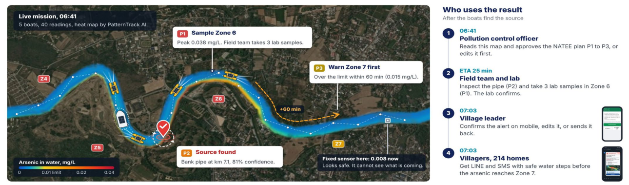
Figure 2.
Example scenario: width 123 m, depth 2.6 m, velocity 0.35 m/s; outfall on bank 2 at km 3.4 (black triangle); full-mixing length 66 km. The dashed line marks the 0.01 mg/L limit; red points are samples above the limit (shown without sensor error). (a) One-bank stations and (b) the centreline boat find no exceedance, whereas (c) the zigzag boat finds seven, all on the outfall bank.
Figure 2.
Example scenario: width 123 m, depth 2.6 m, velocity 0.35 m/s; outfall on bank 2 at km 3.4 (black triangle); full-mixing length 66 km. The dashed line marks the 0.01 mg/L limit; red points are samples above the limit (shown without sensor error). (a) One-bank stations and (b) the centreline boat find no exceedance, whereas (c) the zigzag boat finds seven, all on the outfall bank.
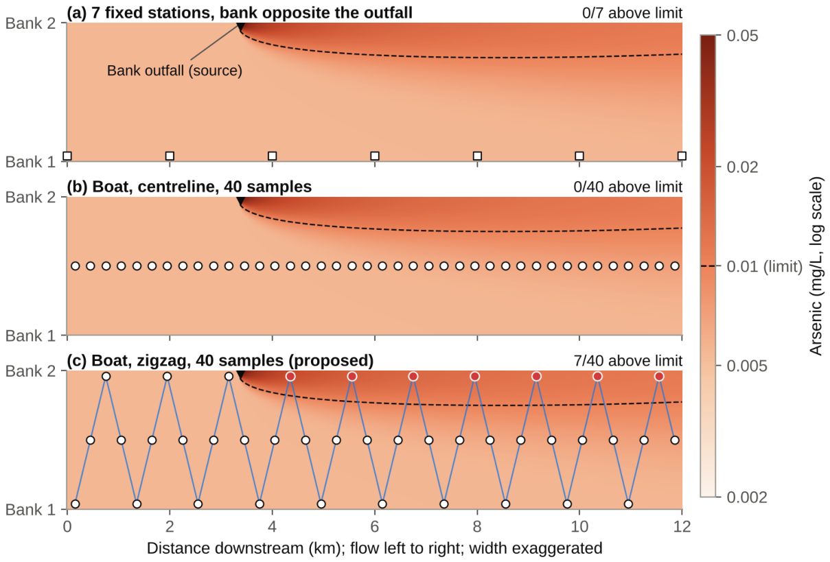
Figure 3.
(a) Detection rate and (b) median source-location error over detected scenarios (log scale) for each sampling design, from 1,776 polluted scenarios. Grey: designs that do not cross the channel; blue: zigzag boat; dark blue: zigzag with bank follow-up.
Figure 3.
(a) Detection rate and (b) median source-location error over detected scenarios (log scale) for each sampling design, from 1,776 polluted scenarios. Grey: designs that do not cross the channel; blue: zigzag boat; dark blue: zigzag with bank follow-up.
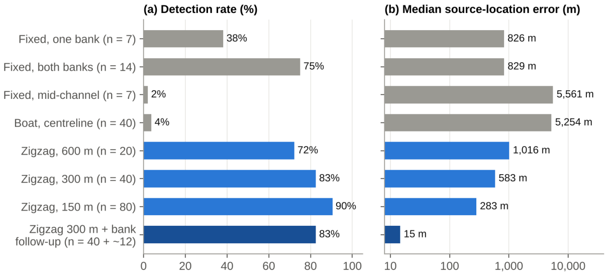

Table 1.
Parameter ranges of the simulated scenarios (uniform unless stated).
| Parameter | Range |
|---|---|
| Width W | 60–150 m |
| Depth d | 1–3 m |
| Velocity U | 0.3–0.9 m/s |
| Friction factor f | 0.02–0.10 |
| Mixing constant α | 0.3–0.9 (sensitivity analysis: 0.6–2.5) |
| Background Cb | 0.002–0.006 mg/L |
| Fully mixed excess concentration | 0.0005–0.005 mg/L (log-uniform) |
| Outfall position xs | km 1–9 |
| Outfall bank | either bank, 50:50 |
| Arsenic limit | 0.01 mg/L |
Table 2.
Results for 1,776 polluted scenarios (α = 0.3–0.9).
| Sampling design | Samples | Detection | Median error | P90 error |
|---|---|---|---|---|
| Fixed stations, one bank | 7 | 38.2% | 826 m | 1,761 m |
| Fixed stations, both banks | 14 | 75.1% | 829 m | 1,742 m |
| Fixed stations, mid-channel | 7 | 2.1% | 5,561 m | 9,801 m |
| Boat, centreline | 40 | 3.8% | 5,254 m | 7,970 m |
| Boat, zigzag 600 m | 20 | 72.2% | 1,016 m | 2,115 m |
| Boat, zigzag 300 m (NEXUSFlow) | 40 | 82.6% | 583 m | 1,075 m |
| Boat, zigzag 150 m | 80 | 90.5% | 283 m | 531 m |
| Boat, zigzag 300 m + bank follow-up | 40 + ~12 | 82.6% | 15 m | 96 m |
Disclaimer/Publisher’s Note: The statements, opinions and data contained in all publications are solely those of the individual author(s) and contributor(s) and not of MDPI and/or the editor(s). MDPI and/or the editor(s) disclaim responsibility for any injury to people or property resulting from any ideas, methods, instructions or products referred to in the content. |
© 2026 by the authors. Licensee MDPI, Basel, Switzerland. This article is an open access article distributed under the terms and conditions of the Creative Commons Attribution (CC BY) license.
Copyright: This open access article is published under a Creative Commons CC BY 4.0 license, which permit the free download, distribution, and reuse, provided that the author and preprint are cited in any reuse.